Sparse feature learning for multi-class Parkinson’s disease classification

2.1Dataset

The data used in this paper is acquired from the Parkinson’s progression markers initiative (PPMI) database.11 PPMI is the first world-wide collaboration of researchers, sponsors, and research participants committing to identify progressive biomarkers to improve PD treatment [13]. They are dedicated to build standardized protocols for acquisition, analysis of the data and to promote the overall comprehension of PD.

Since MRI and DTI images can reveal the detailed structure of the brain, we choose them to provide rich and complementary information in our experiment. MRI image is obtained in the form of a T1-weighted, 3D sequence (i.e., MPRAGE) via Siemens MAGNETOM Trio 3.0T MRI scanners. Then we collect 56 NC, 123 PD, and 29 SWEDD scans. DTI images were selected with the following parameters: slice thickness = 2, flip angle = 90∘, pulse sequence = echo planar (EP), registration = T1, and gradient directions = 64.

Apart from the baseline MRI, DTI data from 208 subjects, we also collect three cerebrospinal fluid (CSF) biomarkers and clinical scores including sleep scores, olfaction scores, depression scores, and MoCA (Montreal Cognitive Assessment) scores to boost performance. The three CSF biomarkers are amyloid beta (1-42) (Aβ1-42), total tau (t-tau) and tau protein phosphorylated at the threonine 181 position (p-tau181). These clinical assessment scores and neuroimaging results can boost the prediction accuracy of our proposed method.

Since smell dysfunction occurs 90% of cases with PD, the olfaction scores are essential for diagnosis. Scores are obtained from the University of Pennsylvania smell identification test (UPSIT), which is commercially accessible for determining certain individual’s olfactory ability. Lower olfaction score means weaker olfactory function. The MoCA scores are generated in a brief 30-question test by a group at McGill University that assesses different types of cognitive abilities. The clinical details of experimental subjects are listed in Table 1.

2.2Preprocessing

All the MRI and DTI images are initially preprocessed by discarding the noise in the images. We select the nonlinear spatial filtering for denoising to improve the performance. In addition, feature extraction, registration and image fusion is also applied. We perform the anterior commissure-posterior commissure (ACPC) correction using COM algorithm to get a better angle. We use the statistical parametric mapping (SPM)22 to correct geometrical distortion and head motion. Finally, the images are processed by skull-stripping for later operation.

For MRI data, we segment the image and group the tissue into gray matter (GM), white matter (WM) and CSF by the SPM default tissue probability maps. These tissues are the main elements of the central nervous system and can help us to analyze neuronal cell changes. To obtain a higher resolution, all images are then re-sampled until isotropic resolution reaches 1.5 mm after normalization and segmentation. Following the automated anatomical labeling (AAL) atlas, we get 116 region-of-interests (ROIs) in the brain. Then we compute the mean tissue density value of these three tissues in each region and use them as features. For DTI data, we further achieve alignment between structural MRI and DTI, and incorporate affine image registrations based on a cost function weighting using FLIRT.33 Specifically, the DTI data is registered to the T1-weighted structural MRI by an affine transformation [14].

DTI images are based on the movement of water molecule. The fractional anisotropy (FA) coefficient of water molecule movement can reflect structural and functional information. The detailed procedures for calculating FA values are illustrated in DTI preprocessing manual.44 For MRI images, we collect 116 GM and 116 WM and 116 CSF tissue volumes for each subject. For DTI images, we obtain 16 mean FA intensity values for each subject. Additional CSF biomarkers and clinical scores are added as complementary features for later use.

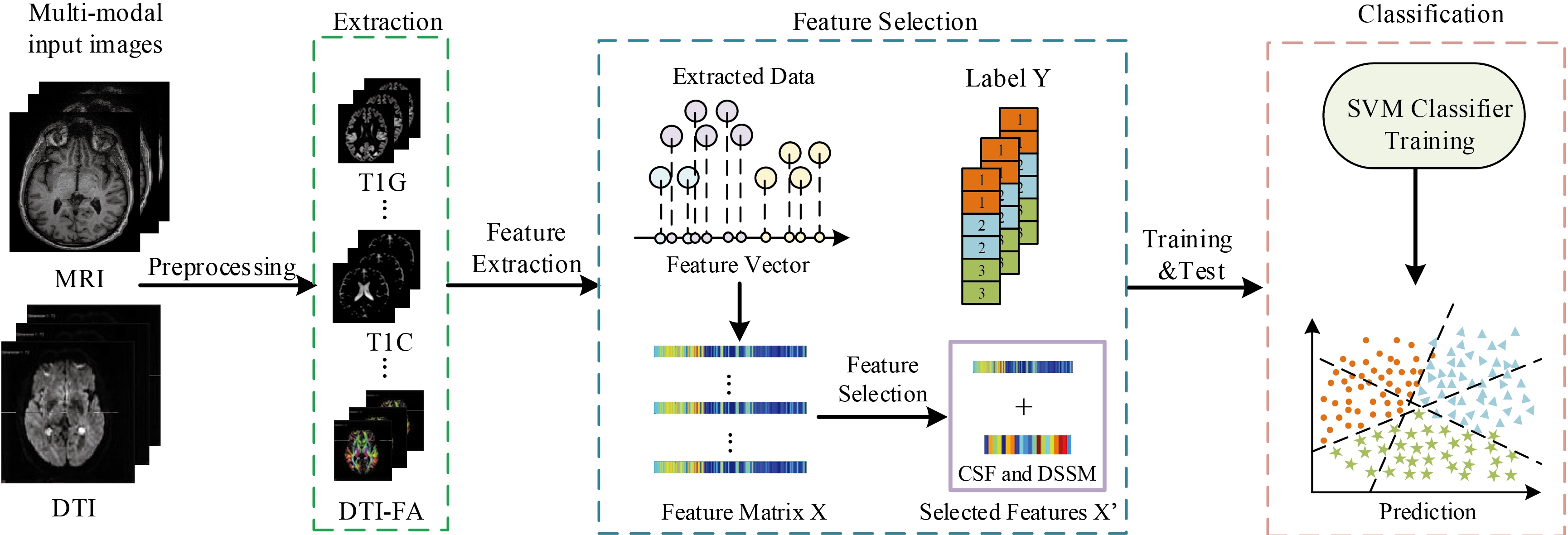
Figure 1.

Flowchart of our method, where T1G is GM of MRI images, T1C stands for CSF of MRI images, DTI-FA stands for FA values of DTI images.

3.1Overview of the method

The overview of our multi-class classification method is presented in Fig. 1. First, we preprocess the original data and extract the tissue volume in the segmented regions to construct GM, CSF, DTI. Then we perform feature selection to get most important features. Specifically, we add CSF biomarkers and clinical scores to the selected features to build our final feature matrix for training the classifiers. We train the classifiers in a supervised manner. Finally, we use support vector classification (SVC) to classify the samples into 3 different groups.

3.2Sparse discriminative feature selection

High dimensionality and small sample size have always been a bottleneck in brain image analysis. Traditionally, the problem of high dimensionality in original data is always settled by a series of dimension reduction methods, e.g., Principal Component Analysis (PCA), Locally Linear Embedding (LLE) [15], LDA [16], Isometric Feature Mapping (ISOMAP) [17]. All these methods can be split into two categories: feature selection and subspace learning [18]. In our method, we jointly perform a feature selection to put them together for further processing. Specifically, we construct a regularized least square regression model based on the idea of Fisher’s LDA combined with LPP, which takes both global and local information into account [19, 20]. Subspace learning methods such as LDA and LPP can convert the initial feature matrix to a feature matrix with reduced dimensionality [21]. By the sparse regularized linear regression model, the most discriminative and relevant features are collected to enhance the classification performance.

In this paper, we denote 𝐗∈𝐑m×d as a feature matrix, and 𝐘∈𝐑m×c as a class matrix, where m, d and c are the size of samples, dimension of features and size of classes respectively. We further introduce Frobenius norm of matrix 𝐗, ∥𝐗∥F=∑i∥𝐱𝐢∥22, and ℓ2,1-norm of 𝐗, ∥𝐗∥2,1=∑i∥𝐱𝐢∥2. In general, a linear prediction model can be defined as follows:

where 𝐖∈𝐑d×c represents a regression coefficient matrix. The first term controls the overall data fitting error. The second term ensures the sparsity level of 𝐖 and λ is the hyperparameter. However, it only selects the smallest number of features and fails to select the most related features. Hence, we utilize the neighborhood structure of the original data to tackle this problem. First, we use the Fisher’s LDA to consider the global information to find the most relevant features [20]. Following the Fisher’s criterion [22], we add a regularization term, defined as follows:

where ∑w represents the within-class variance and ∑b is the between-class variance. Maximizing this ratio ensures that we get 𝐖 with relatively small within-class variance and relatively large between-class variance. Although it is hard to find a solution in Eq. (2), another way can be found to maximize it by equivalently defining the class matrix as follows:

where 𝑙𝑎𝑏𝑒𝑙⁢(𝐱i) is the label of the sample 𝐱i, mk is the sample amount of class k. As a result, we can utilize the global information of data. For the relation between data, LPP is used to maintain the relation within data [23]. We use the graph Laplacian method to define the similarity Si,j between sample 𝐱i and 𝐱j and define a regularization term as follows:

where 𝐒=[Si,j]m×m denotes the affinity matrix of data samples. In LPP, it first constructs a neighborhood graph for data 𝐗 using K-Nearest-Neighbor (KNN) and then computes the value of 𝐒 by making the sum of each row equals to one. Then our final objective function is

where λ1 and λ2 are regularization parameters. Therefore, we can jointly combine subspace learning and feature selection. Hence, we calculate the ℓ2-norm value of each row vector in 𝐖 and each feature has a representative weight value. Then the features are selected by a threshold value. Specifically, the average weight value of all features is calculated as the threshold to adjust the feature accordingly. The weight of features less than the threshold value will be set to zero. The threshold value can be adjusted according to average weight. Using the collected information, we can train the regression model to select the most discriminative features with limited size.

Inspired by [24], we solve Eq. (5) by the accelerated proximal gradient method to iteratively update the value of 𝐖 and ignore the part unrelated with 𝐖. Then we can find the optimal 𝐖 with a closed form of solution [24].

3.3SVM classification

Differing from the preceding methods that merely perform a binary classification, a multi-class classification is adopted for PD diagnosis in our method. In machine learning, SVM is a supervised learning model used for pattern recognition, classification and regression analysis. The main idea of SVM is finding the best hyperplane that can separate different class samples with the maximum margin. Hence, we choose the SVM to construct a multi-class classification model. The free and available software libsvm55 toolbox (version: libsvm-2.91) is used to perform the classification task.

In binary SVM classification, we directly make use of the outputs of the prediction function. In multi-class classification, the output of SVM prediction will change, for example, the dimension of decision values is equal to the number of all possible binary classification combinations. For samples belonging to k class, we can select all the binary combination. Then a total of n×(n-1)/2 classification models are built. The final performance of multi-class is obtained from the best result.

4.1Experimental settings

In our experiments, we perform the multi-class classification NC vs. PD vs. SWEDD via SVM. In the 10-fold cross-validation method, for each subset of experiment, we train feature selection model by different feature combination sets, i.e., GM of MRI (T1G for short), WM of MRI (T1W for short), CSF of MRI (T1C for short), FA of DTI (DTI for short), T1G + T1C + DTI (GCD for short), T1W + T1C + DTI (WCD for short), and T1G + T1W + T1C + DTI (GWCD for short). After the feature selection, we add CSF biomarkers (CSF for short) and clinical scores (DSSM for short) to the selected feature matrix. For each feature set, a classification model is obtained to get the class labels.

Figure 2.

Classification accuracy of various hyperparameters (λ1 and λ2).

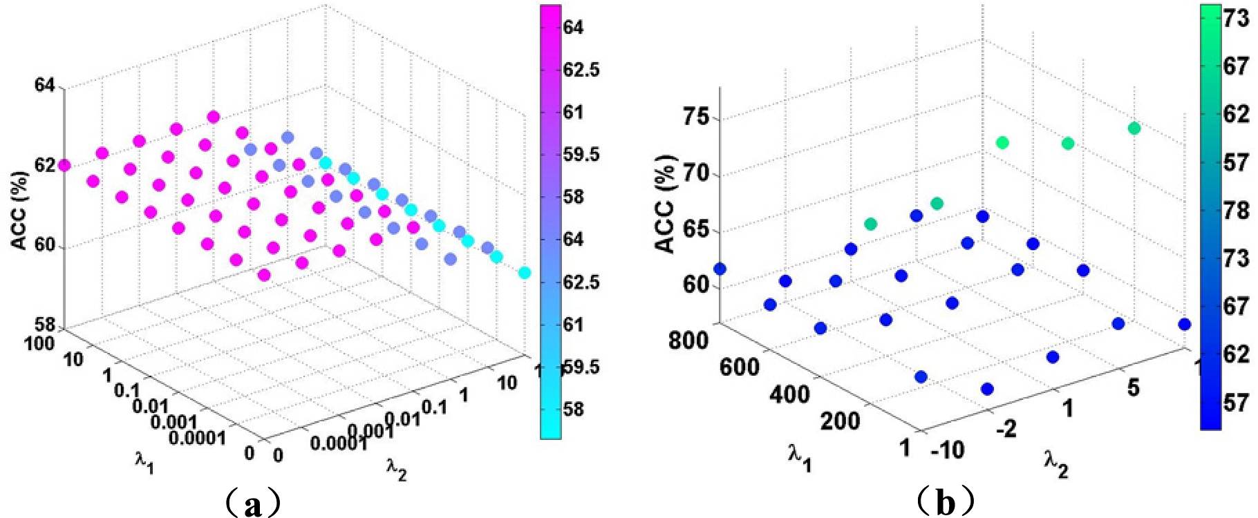
4.2Parameters

The main parameters used in our method is the feature selection tuning parameters in Eq. (4), λ1 and λ2. Its initiation values are as below: λ1∈{10-5,…,102}, λ2∈{10-5,…,102}. The final values can be specified by altering the value until the overall performance reaches the peak. Figure 2 shows the effect of λ1 and λ2 on the whole process. We can clearly see the peak value. To achieve better performance and get more specific parameters, we further shorten the step size and the range, which is illustrated in Fig. 2b, the most suitable parameters can be selected when there is no variation in the accuracy values. It is clear that the regularization parameters can affect the classification accuracy, the final results can only be achieved by tuned parameters in several iterations. We set λ1=200 and λ2=1 as the tuned parameters. As for the C, G parameters of SVM classification, in each 100 iterations, we automatically chose the result with the highest AUC value and save the corresponding C and G values.

4.3Classification results

In the experiments, we use quantitative measurements to evaluate the performance of our method. These measurements include accuracy (ACC), sensitivity (SEN), precision (PREC), F-scores (F1), area under the receiver operating characteristic curve (AUC). Table 2 shows the multi-class classification results of NC vs. PD vs. SWEDD from single modality to multimodal data. Before deciding what features combine together can produce the best results, we perform different sets of feature groups and compare the outputs. We can clearly see that the single modality using only one type of features (T1G, T1W, T1C, DTI) is slightly worse than other combination groups. We noticed that T1W has the least effectiveness as well as the combination including T1W. Among all these combination modes, we select the one with the highest accuracy. Accordingly, we use the GCD combination as the feature matrix before feature selection process. Apart from these features, we add three CSF biomarkers and four clinical scores to the feature matrix before training SVM classifiers. Since these features only take a small proportion in the original data, they have no need for feature selection process. The achieved performance proves that our strategy of adding CSF biomarker and clinical scores boost the classification results. The classification performance with multi-modality features (GCD) combined with CSF and DSSM is always better than those without additional features. Therefore, the combination GCD + CSF + DSSM is selected as the final feature matrix for training a SVM classifier.

Figure 3.

ROC results for comparison between other competing methods.

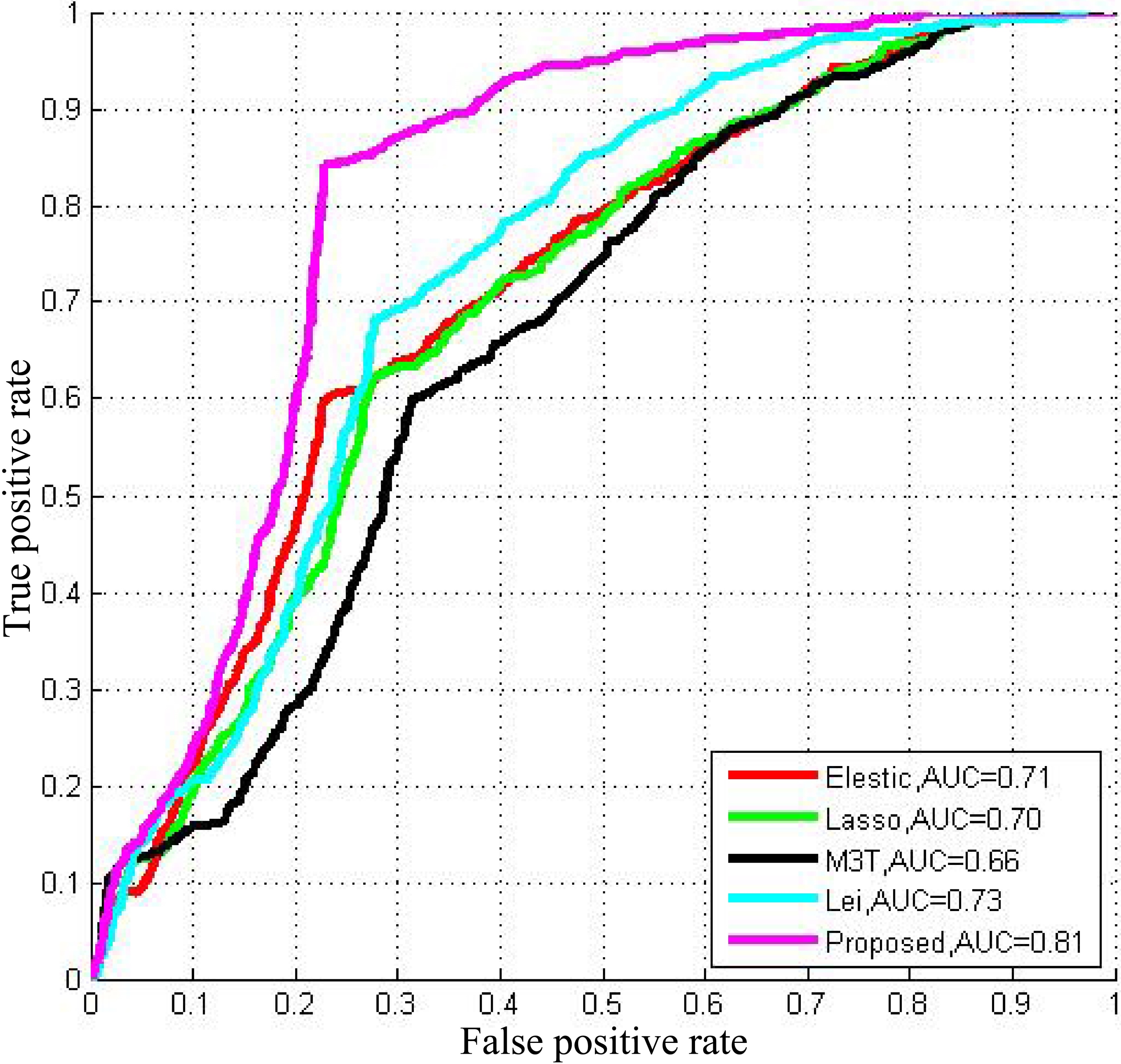
We compare our proposed method with other widely used methods such as elastic net, least absolute shrinkage and selection operator (Lasso) [26], Multi-modal multi-task (M3T) [1], Lei et al.’s [27]. Receiver operating characteristic (ROC) curves based on 100 times cross-validation of comparison among these competing methods and our proposed method are demonstrated in Fig. 3. We observe that the proposed method is superior to competing methods using the organized features. Overall, the proposed method achieves an accuracy of 78.4%, a sensitivity of 84.7%, a precision of 66.7%, an F1 score of 70.2% and an AUC of 94.2% with multi-modality data. Details are illustrated in Table 3. The proposed method with GCD + CSF + DSSM features clearly has remarkable performance.

In our experiment, we combined different features before and after the feature selection. As shown in Table 3, the experimental results demonstrate that our feature selection method enhances the classification performance. We also find that the proposed sparse feature selection method based on multi-modal data outperforms competing methods. Furthermore, our multi-class classification can classify the samples into three categories and shows the efficacy of our proposed method.

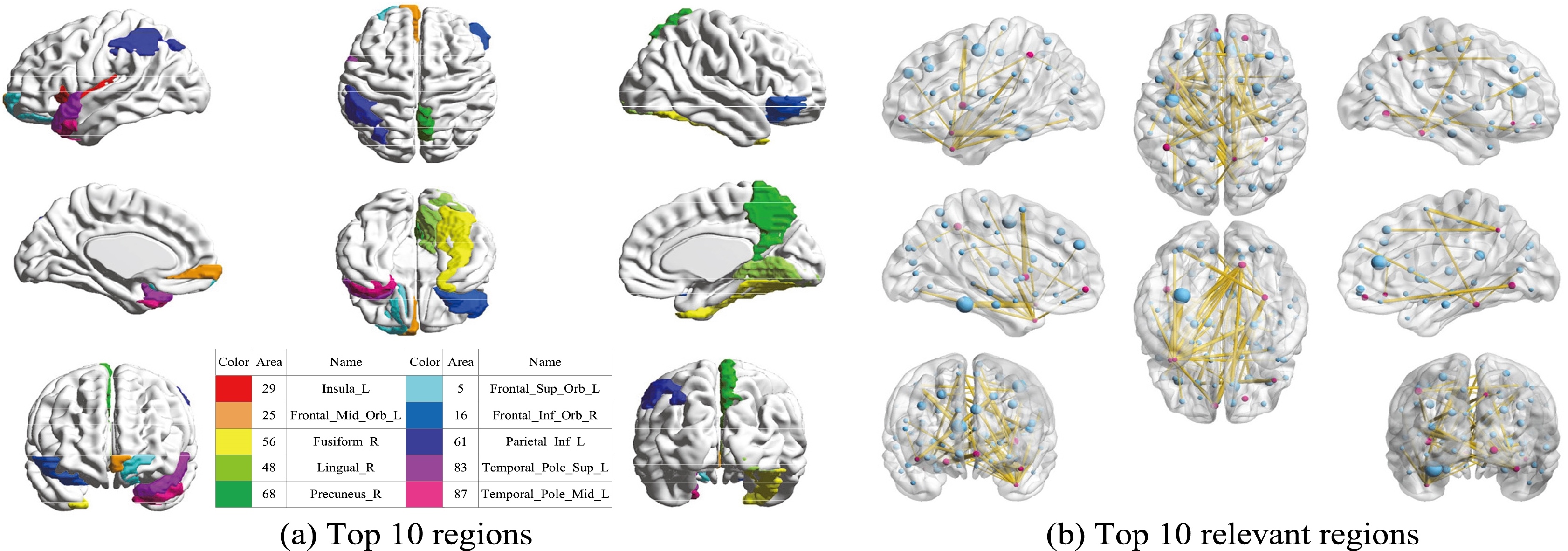
Figure 4.

(a) Top 10 discriminative brain regions obtained from proposed method via for NC vs. PD vs. SWEDD. Brain regions were color-coded. (b) Top 10 relevant brain regions (in blue points) for each top 10 discriminative brain region (in red points).

4.4Related brains regions

Our experiments are based on the assumption that GM or WM or other brain biomarkers are changed. To better facilitate early diagnosis and monitoring the progression of PD for the corresponding treatments, we also studied the relevant and discriminative brain regions about PD. To find the top 10 regions, we utilize the weight coefficient matrix produced in feature selection process through a 10-fold cross validation method. The weight matrices present the significance of all the 116 brain regions. We choose the top 10 regions with the highest weight value in a descending order and delete the repeat regions. The top 10 relevant brain regions selected from multi-class classification are visualized in Fig. 4. Moreover, suffix ‘_L’ indicates the left brain, suffix ‘_R’ indicates the right brain, and different colors indicate different brain regions. The top 10 brain regions recognized with GCD multi-modal features using our proposed method are insula left, middle frontal gyrus (orbital part), fusiform gyrus right, lingual gyrus right, precuneus right, superior frontal gyrus (orbital part), inferior frontal gyrus (orbital part), inferior parietal (but supramarginal and angular gyri), temporal pole (superior temporal gyrus), middle temporal gyrus. To further study the relationship between brain regions and PD, we continue with in-depth study on the top 10 regions by seeking the other top 10 brain regions which have the most correlation with the selected top 10 regions. We use the same weighting matrix as selecting top 10 regions to calculate the Pearson correlation coefficient to represent the correlation among different regions. The weighting coefficient is used to select the 10 other relevant regions of each top 10 brain regions. The results are also visualized in Fig. 4, and the red points in each image represents the top 10 ROIs, and each red point spreads 10 yellow lines to connect 10 other points in blue which indicates the 10 relevant ROIs.

References

[1] | Zhang D, Shen D. Multi-modal multi-task learning for joint prediction of multiple regression and classification variables in Alzheimer’s disease. Neuroimage (2012) ; 59: (2): 895-907. |
[2] | Postuma RB, Berg D, Stern M, Poewe W, Olanow CW, Oertel W, et al. MDS clinical diagnostic criteria for Parkinson’s disease. Movement Disorders (2015) ; 30: (12): 1591-1599. |
[3] | Braak H, Del TK, Rüb U, de Vos RA, Jansen Steur EN, Braak E. Staging of brain pathology related to sporadic Parkinson’s disease. Neurobiology of Aging (2003) ; 24: (2): 197-211. |
[4] | Willis AW, Schootman M, Kung N, Racette BA. Epidemiology and neuropsychiatric manifestations of young onset Parkinson’s disease in the United States. Parkinsonism and Related Disorders (2013) ; 19: (2): 202-206. |
[5] | Prashanth R, Dutta Roy S, Mandal PK, Ghosh S. Automatic classification and prediction models for early Parkinson’s disease diagnosis from SPECT imaging. Expert Systems with Applications (2014) ; 41: (7): 3333-3342. |
[6] | Lei B, Jiang F, Chen S, Ni D, Wang T. Longitudinal analysis for disease progression via simultaneous multi-relational temporal-fused learning. Frontiers in Aging Neuroscience (2017) ; 9: (6). |
[7] | Adeli E, Shi F, An L, Wee C-Y, Wu G, Wang T, et al. Joint feature-sample selection and robust diagnosis of Parkinson’s disease from MRI data. NeuroImage (2016) ; 141: : 206-219. |
[8] | Fung G, Stoeckel J. SVM feature selection for classification of SPECT images of Alzheimer’s disease using spatial information. Knowledge and Information Systems (2007) ; 11: (2): 243-258. |
[9] | Rana B, Juneja A, Saxena M, Gudwani S, Kumaran S, Behari M, et al. A machine learning approach for classification of Parkinson’s disease and controls using T1-weighted MRI. Movement Disorders (2014) ; 29: : S88-S89. |
[10] | Salvatore C, Cerasa A, Castiglioni I, Gallivanone F, Augimeri A, Lopez M, et al. Machine learning on brain MRI data for differential diagnosis of Parkinson’s disease and progressive supranuclear palsy. Journal of Neuroscience Methods (2014) ; 222: : 230-237. |
[11] | Shin HC, Roth HR, Gao M, Lu L, Xu Z, Nogues I, et al. Deep convolutional neural networks for computer-aided detection: CNN architectures, dataset characteristics and transfer learning. IEEE Transactions on Medical Imaging (2016) ; 35: (5): 1285-1298. |
[12] | Aerts MB, Esselink RA, Post B, Bp VDW, Bloem BR. Improving the diagnostic accuracy in parkinsonism: A three-pronged approach. Practical Neurology (2012) ; 12: (2): 77-87. |
[13] | Marek K, Jennings D, Lasch S, Siderowf A, Tanner C, Simuni T, et al. The Parkinson progression marker initiative (PPMI). Progress in Neurobiology (2011) ; 95: (4): 629-635. |
[14] | Tao R, Fletcher PT, Gerber S, Whitaker RT. A variational image-based approach to the correction of susceptibility artifacts in the alignment of diffusion weighted and structural MRI. Information Processing in Medical Imaging (2009) ; 21: : 664-675. |
[15] | Ridder DD, Kouropteva O, Okun O, Pietikäinen M, Duin RPW. Supervised locally linear embedding. Springer Berlin Heidelberg; (2003) . |
[16] | Yang S, Zhao C. A fusing algorithm of Bag-Of-Features model and Fisher linear discriminative analysis in image classification. (2012) ; 380-383. |
[17] | Maaten LJPVD, Postma EO, Herik HJVD. Dimensionality reduction: A comparative review. Journal of Machine Learning Research (2009) ; 10: (1): 66-71. |
[18] | Ghodsi A. Dimensionality reduction a short tutorial. General Information (2006) ; 22: (2): 183-207. |
[19] | Zhang L, Qiao L, Chen S. Graph-optimized locality preserving projections. Pattern Recognition (2010) ; 43: (6): 1993-2002. |
[20] | Balakrishnama S, Ganapathiraju A. Linear discriminant analysis – a brief tutorial. Proc of the Int Joint Conf on Neural Networks (1998) ; 3: (94): 387-391. |
[21] | Lei B, Yang P, Wang T, Chen S, Ni D. Relational-regularized discriminative sparse learning for Alzheimer’s disease diagnosis. IEEE Transactions on Cybernetics (2017) ; 47: (4): 1102-1113. |
[22] | Kotsia I, Zafeiriou S, Pitas I. Novel multiclass classifiers based on the minimization of the within-class variance. IEEE Transactions on Neural Networks (2009) ; 20: (1): 14-34. |
[23] | Dai G, Yeung DY. Tensor embedding methods. National Conference on Artificial Intelligence and the Eighteenth Innovative Applications of Artificial Intelligence Conference 16-20 July 2006, Boston, Massachusetts, USA, (2006) . |
[24] | Nesterov Y. Introductory lectures on convex optimization. Applied Optimization (2004) ; 87: (5): xviii, 236. |
[25] | Chui KT, Tsang KF, Chi HR, Ling BWK, Wu CK. An accurate ECG-based transportation safety drowsiness detection scheme. IEEE Transactions on Industrial Informatics (2016) ; 12: (4): 1438-1452. |
[26] | Tibshirani RJ. Regression shrinkage and selection via the LASSO. Journal of the Royal Statistical Society (1996) ; 58: (1): 267-288. |
[27] | Lei H, Huang Z, Zhang J, Yang Z, Tan EL, Zhou F, et al. Joint detection and clinical score prediction in Parkinson’s disease via multi-modal sparse learning. Expert Systems with Applications (2017) ; 80: (1): 284-296. |