
Epileptic seizure detection based on the kernel extreme learning machine
Abstract
This paper presents a pattern recognition model using multiple features and the kernel extreme learning machine (ELM), improving the accuracy of automatic epilepsy diagnosis. After simple preprocessing, temporal- and wavelet-based features are extracted from epileptic EEG signals. A combined kernel-function-based ELM approach is then proposed for feature classification. To further reduce the computation, Cholesky decomposition is introduced during the process of calculating the output weights. The experimental results show that the proposed method can achieve satisfactory accuracy with less computation time.
1.Introduction
Epilepsy is one of the most common chronic neurological disorders worldwide. The hyper-synchronized causes excessive electrical discharges in a group of neurons. Approximately one in every 100 people is afflicted by it [1]. EEG recorded by electrodes placed on the scalp is an efficient method for checking electrical activity in the brain. Conventional diagnosis of neurological disorders based on EEG signals relies on neurologists to visually check the recordings; it is experience-dependent and time-consuming. Therefore, to reduce the artificial workload and improve the efficiency and accuracy of the diagnosis, the application of signal processing and machine learning methods for epileptic EEG signal analysis is valuable.
The process of automatic epileptic seizure analysis is a pattern recognition system that can distinguish seizures from standard EEG signals [2]. In recent years, many problems have been solved, with relevant methods. Suitable features are essential for correct detection of epileptic patterns. To date, temporal [3], frequency [4], wavelet [5], spatial [6], nonlinear dynamic, and deterministic chaos features, as well as multi-feature fusion strategies [7], have been used to describe EEG signals [8, 9]. In addition, many effective classification algorithms have been used in this area, such as support vector machine (SVM) [10, 11], artificial neural networks (ANN) [12], etc. Some of the methods have achieved satisfactory performance. Especially, work [11] has obtained extraordinary recognition accuracy.
However, owing to the poor signal-to-noise ratio (SNR) of raw EEG signals in practical application, the problems of improving recognition performance and identification efficiency still exist. The limits existing in conventional methods including overlong training time, unsatisfactory accuracy or limited generalization performance for clinical application make the automatic detection of epileptic seizure still challenged. Compared with other algorithms, the ELM requires less training time while maintaining satisfactory classification accuracy. Problems existing in traditional feedforward neural network learning algorithms such as local minima and various training parameters are avoided in ELM. Furthermore, it has a higher generalization performance. Owing to its superior property, ELM has thus been applied to EEG signal feature classification based on diverse feature extraction methods and has achieved impressive performance in literatures [5, 13, 14] for instance.
To better balance the conflict between efficiency and accuracy of pattern recognition, this paper focuses primarily on the classification process for seizure recognition. In the proposed algorithm, several features are combined comprehensively to represent the characteristics of EEG for epilepsy. Then a combined kernel function is introduced into ELM. Moreover, Cholesky decomposition is employed to reduce the calculation burden and the effectiveness of the algorithm, validated through experiments.
2.Kernel elm based on cholesky decompositon
Unlike conventional single hidden layer feed forward neural networks (SLFNs), the parameters of hidden layers in ELM are randomly given at the beginning of the training process and fixed it instead of the complicated iterative calculation process. Then, the least-squares method is used to obtain the output weights [15].
Otherwise, ELM tends to minimize the training error and the norm of production weights. The introduction of kernel function gives the algorithm more stability and better generalization ability [16]. All the above attributes give the kernel ELM higher efficiency and better performance [17].
2.1Kernel ELM
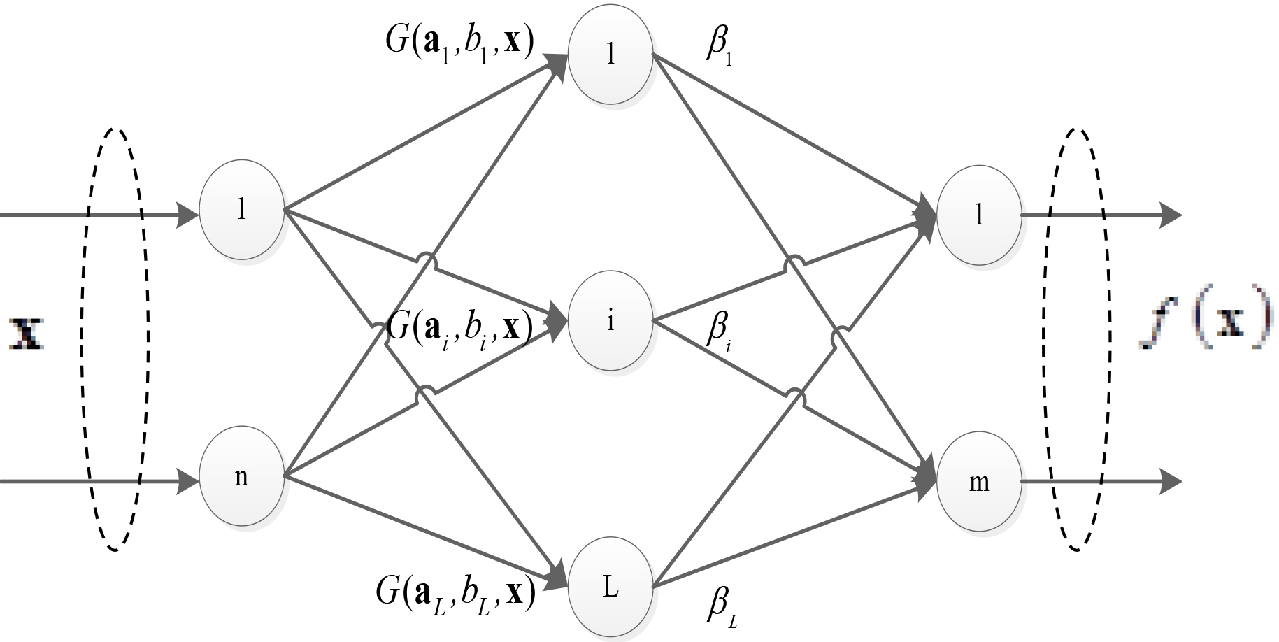
Suppose there are
(1)
Figure 1.
Single hidden layer feedforward network.
Where
The least-squares method is utilized to obtain weight
(2)
The unique solution is
(3)
Where
(1) Randomly assign input weights
(2) Calculate the hidden layer output matrix
(3) Obtain the output weights according to Eq. (3).
If
(4)
where
(5)
If the hidden layer feature mapping
(6)
Thus, Eq. (5) can be written as:
(7)
Then, we have:
(8)
For binary classification, the class label is determined by the two outputs of ELM through a competition mechanism. For the multi-class problem, the number of products should be the same as the number of categories. The output with the maximum value is the class to which the sample belongs.
2.2ELM based on Cholesky decomposition
In this paper, Cholesky decomposition is used to decrease the computation burden in the process of obtaining the output weights. This factorization method factorizes a matrix into the product of a triangular matrix and its conjugate transpose matrix.
The expression of the output weights rewrote as:
(9)
Assuming that
(10)
Then we have
(11)
Apparently,
(12)
For any
(13)
where
where
(14)
Thus, Eq. (11) can be written as:
That is,
(15)
Assuming
(16)
(17)
The output weights,
(18)
Unlike conventional ELM calculations of the inverse matrix, this method directly obtains the output weights by iterative computations on Eqs (14), (17) and (18). These formulas involve only addition, subtraction, and square root operations; thus, the computational complexity is significantly reduced.
2.3Online update scheme
For the characteristic calculation based on Cholesky decomposition, it is convenient to extend the algorithm to the practical application of detecting epileptic seizures in routine clinical EEG recordings online.
When a new sample arrives, the matrix of the hidden layer can be written as:
Thus,
(19)
For the introduction of the kernel function,
(20)
Through Eq. (14), it is evident there no need to recalculate the 1-N rows and the 1-N columns of
3.Method
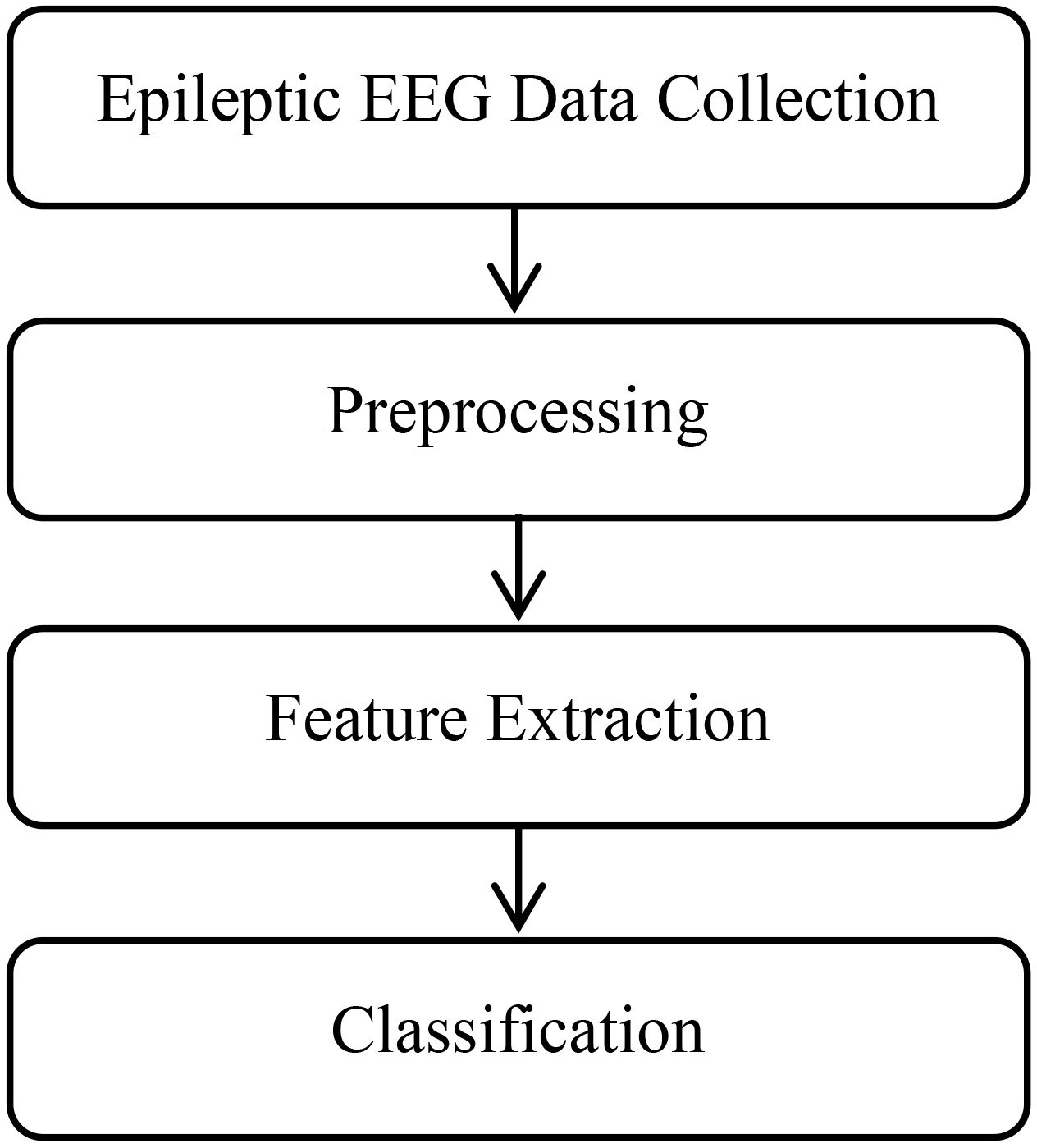
The flowchart of the recognition system mainly includes data collection, preprocessing, feature extraction, and classification (cf. Fig. 2).
Figure 2.
Flowchart of epileptic EEG recognition.
3.1Preprocessing
Original EEG signals pollute various interference signals, such as power line interference and electrooculograms (EOGs). To eliminate the effect of noise and to obtain cleaner EEG signals, preprocessing is necessary. Preprocessing steps commonly include filtering, data normalizing, artifact rejecting, etc. According to actual needs, reasonable measures can then be selected.
Waves with useful information are predominantly distributed in low-frequency regions. Therefore, for our application requirement, a six-order band-pass Chebyshev Type I filter with cutoff frequencies of 0.5 Hz and 40 Hz was designed to filter each extracted signal. This process comprised the first step of the analysis.
3.2Feature extraction
The purpose of the feature extraction process is to find compelling features to characterize the cognitive components. The extracted feature vectors of different tasks are expected to have distinct differences. Multiple elements are removed, from various EEG signals, including time domain features, wavelet packet energy, and entropy. The mathematical expressions of several featured used are:
(1) Crest Factor
(2) Kurtosis
(3) Impulse Factor
(4) Signal Factor
The above listed time domain features are the most intuitive and straightforward ways to observe and analyze signals. However, for complex EEG signals with characteristics of nonlinearity, nonstationarity, and time variation, a single analysis method often cannot obtain a good effect. Therefore, we chose wavelet packet decomposition (WPD), which can efficiently locate signals in both time and frequency domains to extract the EEG features [18].
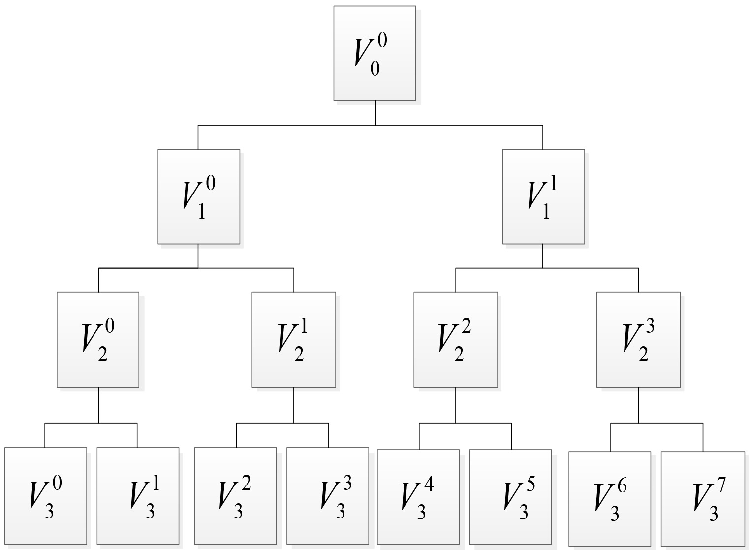
As shown in Fig. 3, through wavelet packet transformation, each epoch is decomposed into three levels. Eight sets of coefficients in the following frequency bands are obtained: 0.5–5 Hz, 5–10 Hz, 15–15 Hz, 15–20 Hz, 20–25 Hz, 25–30 Hz, and 35–40 Hz.
Figure 3.
The structure of WPD,
Then, the wavelet packet energy and entropy of each node are calculated as features of the EEG signals. They respectively indicate the strength and complexity of signals. The power of the EEG signal of a finite length is given by
(21)
where
(22)
The wavelet packet entropy is calculated according to Eq. (3.2), where the Shannon entropy is employed.
(23)
Thus, the entropy feature vector of each epoch is:
(24)
Consequently, the feature vector of each time is constructed as follows.
(25)
3.3Classification
Any function can be used as the kernel function of ELM as long as it aligns with Mercer’s theorem [19]. Several commonly used core functions exist, including the respective Gaussian kernel, polynomial kernel, perceptron kernel, radial basis function (RBF) kernel, wavelet kernel functions, among others. They each offer different advantages. Whether the selection of basic function is reasonable will directly affect the final classification result. A separate service often cannot achieve a satisfactory approximation effect. Accordingly, a combined kernel function, which is expected to obtain a better result, is constructed by adding different weights to different core roles in this study.
Here, the RBF kernel function, which has a stronger learning capability, and the polynomial kernel function, which offers a better generalization ability, are adopted to construct the combined core function. The expressions are as follows.
(1) RBF kernel function:
(2) Polynomial kernel function:
Thus, the combined primary function is:
(26)
Where
After the initialization, differential evolution (DE) algorithm is adopted to obtain the optimal values of the three parameters (punishment factor
Table 1
Description of the three datasets analyzed
| Datasets | Subject | Electrode type | Subject’s state |
|---|---|---|---|
| Set A | Five healthy subjects | Surface | Normal |
| Set D | Five patients | Intracranial | Seizure-free |
| Set E | Five patients | Intracranial | Seizure activity |
4.Experiments
4.1Data description
The Department of Epileptology, Bonn University, Germany [18] obtained the experimental data applied in this study; collecting from five healthy subjects and five epileptic patients. The complete dataset includes five sets (A-E), three of which are analyzed in this paper (A, D, and E). Details of the three datasets are listed in Table 1.
In each dataset, 100 single-channel EEGs of 23.6 s durations were recorded. The data sampling rate was 173.61 Hz. Thus, each EEG epoch had 4,096 sampling points.
4.2Results
In this section, the classification performance of the proposed algorithm is evaluated on the epileptic EEG datasets described above. A binary classifier was established to distinguish samples among healthy subjects (dataset A) and patients (dataset E). Additionally, the three-class problem among the three datasets was solved. The ten-fold cross-validation technique was used to reduce the bias of training and testing data. According to this technique, the dataset was divided into ten subsets [21]. To improve the dependability of this technique, the 10-fold cross-validation procedure was performed 10 times. Each time, one of the ten subsets was utilized as the testing dataset and the other 9 subsets were put together to form the training dataset. In particular, the data from test fold is not involved in the optimization procedure. All final results were averaged over the ten repetitions.
Tables 2 to 4 show the results. Specifically, Tables 2 and 3 compare the correctly classified percentage and the time required for training of different algorithms in the binary-class problem between health and seizures, and the three-class problem among health, seizure-free, and seizure activity. Moreover, to better inspect the performance, a confusion matrix is shown in Table 4.
Table 2
Comparison of different algorithms for binary problem
| Method | Average classification accuracy (%) | Average training time (s) |
|---|---|---|
| BPNN | 92.2 | 69.82 |
| SVM | 90.3 | 23.15 |
| Original ELM | 94.2 | 0.145 |
| Work [11] | 100 | 59.20 |
| Work [5] | 94.8 | 0.980 |
| Proposed | 97.7 | 0.104 |
Table 3
Comparison of different algorithms for a three-class problem
| Method | Average classification accuracy (%) | Average training time (s) |
|---|---|---|
| BPNN | 90.9 | 80.97 |
| SVM | 88.4 | 34.50 |
| Original ELM | 93.6 | 0.238 |
| Work [11] | 98.2 | 75.70 |
| Work [7] | 96.0 | 80.71 |
| Proposed | 96.5 | 0.157 |
Table 4
Confusion matrix of the proposed method
| Set A | Set D | Set E | |
|---|---|---|---|
| Set A | 100 | 4 | 1 |
| Set D | 0 | 94 | 3 |
| Set E | 0 | 2 | 96 |
4.3Discussion
Tables 2 and 3 show that the average recognition accuracies of our method in binary and three-class problems are both better than SVM, back-propagation (BP) neural network (BPNN), and the original ELM adopted. Because the Cholesky decomposition was adopted to simplify the calculation, our method was more time-efficient compared to SVM, BPNN and the method proposed in literature [11]. From the results, we can see that the proposed algorithm is suitable for the recognition of epileptic EEG patterns.
To apply the practice, there needs to be, no time-consuming operation in our approach. During the process of feature extraction, each epoch is decomposed into three levels by wavelet packet transform. More decomposition levels have no significant effects on the results, which was confirmed by experiments. Also, the classifier model can be quickly refreshed online if demanded (e.g., routine clinical applications). No need exists to retrain the entire network; only some parameters must be calculated (as described in Section 2.3). Through incremental recursion; the new training function can obtain new samples.
About future research, because there are various unpredictable interferences in EEG data collected in complex application environments, more pre-processing operations should be taken into account, such as automatic artifact rejection, to enhance the signal-to-noise ratio. Also, a more efficient feature extraction method, such as deep learning, can be a feasible way to improve the performance of the classifier. Additional experiments on practical applications are required, to address the remaining areas of improvement owing to the complexity of seizure recognition.
5.Conclusions
In this paper, we proposed an ELM kernel algorithm by introducing a combined kernel function to address the problem of seizure recognition. By employing Cholesky decomposition and its calculation process, which involves only arithmetic, the calculation efficiency of the proposed method is further improved.
Among different classifiers, a comparative study was conducted, to illustrate effectiveness in our approach. The results show that our method achieves better recognition accuracy with considerably less training time. The overall implementation of the method is easy to understand, and the computation burden is low.
Conflict of interest
None to report.
References
[1] | Lehnertz K, Mormann F, Kreuz T, Andrzejak RG, Rieke C, David P, CElger CE. Seizure prediction by nonlinear EEG analysis. IEEE mag. Eng. Med. Biol. (2003) : 1: (22): 57-63. |
[2] | Gotman J. Automatic recognition of epileptic seizures in the EEG. Electroencephalogr. Clin. Neurophysiol. (1982) : 54: : 530-540. |
[3] | Srinivasan V, Eswaran C, Sriraam N. Artificial neural network based epileptic detection using Time-domain and frequency-domain features. Journal of Medical Systems. (2003) : 29: (6): 647--660. |
[4] | Übeyli ED. Least squares support vector machine employing model-based methods coefficients for analysis of EEG signals. Expert Systems with Applications. (2010) : 37: : 233-239. |
[5] | Song Y, Zhang J. Automatic recognition of epileptic EEG patterns via extreme learning machine and multi-resolution feature extraction. Expert Systems with Applications. (2013) : 40: (14): 5477-5489. |
[6] | Alotaiby TN, Abd El-Samie FE, Alshebeili SA. Seizure detection with common spatial pattern and Support Vector Machines. Int. Conf. Information and Communication Technology Research. (2015) : 152-155. |
[7] | Acharya UR, Yanti R, Zheng JW. Automated diagnosis of epilepsy using CWT, HOS and texture parameters. International Journal of Neural Systems. (2013) : 23: (3): 1350009. |
[8] | Kannathal N, Acharya UR, Lim CM, Sadasivan PK. Characterization of EEG-A comparative study. Computer Methods and Programs in Biomedicine. (2005) : 80: (1): 17--23. |
[9] | Wang CM, Zou JZ, Zhang J, Wang M, Wang RB. Feature extraction and recognition of epileptiform activity in EEG by combining PCA with ApEn. Cognitive Neurodynamics. (2010) : 4: : 233-240. |
[10] | Nicolaou N, Georgiou J. Detection of epileptic electroencephalogram-based on permutation entropy and support vector machines. Expert Systems with Applications. (2012) : 39: : 202-209. |
[11] | Kumar Y, Dewal ML, Anand RS. Epileptic seizure detection using DWT based fuzzy approximate entropy and support vector machine. Neurocomputing. (2014) : 133: : 271-279. |
[12] | Übeyli ED. Combined neural network model employing wavelet coefficients for EEG signals classification. Digit. Signal Process. (2009) : 19: : 297-308. |
[13] | Song Y, Crowcroft J, Zhang J. Automatic epileptic seizure detection in EEGs based on optimized sample entropy and extreme learning machine. Journal of Neuroscience Methods. (2012) : 210: (2): 132-146. |
[14] | Yuan Q, Zhou WD, Li SF, Cai DM. Epileptic EEG classification based on extreme learning machine and nonlinear features. Epilepsy Research. (2009) : 96: : 29-38. |
[15] | Huang GB, Zhu QY, Siew CK. Extreme learning machine: theory and applications. Neurocomputing. (2006) : 70: (1): 489-501. |
[16] | Huang GB, Zhou H, Ding X, Zhang R. Extreme learning machine for regression and multiclass classification. IEEE Trans. Systems, Man, and Cybernetics, Part B: Cybernetics. (2012) : 42: (2): 513-529. |
[17] | Huang GB, Wang DH, Lan Y. Extreme learning machines: a survey. Int. J. Machine Learning and Cybernetics. (2011) : 2: (2): 107-122. |
[18] | Wu T, Yan GZ, Yang BH, Sun H. EEG Feature Extraction Based on Wavelet Packet Decomposition for Brain-Computer Interface. Measurement. (2008) : 41: (6): 618-625. |
[19] | Cortes C, Vapnik V. Support-vector networks. Mach. Learn. (1995) : 20: (3): 273-297. |
[20] | Storn R, Price K. Differential evolution-a simply and efficient adaptive scheme for global optimization over continuous spaces. Journal of Global Optimization. (1997) : 11: (4): 341-359. |
[21] | Ripley BD. Pattern Recognition and, Neural Networks. Cambridge. K.: Cambridge University Press. (1996) . |


