The curvature calculation mechanism based on simple cell model

1.Introduction

Researchers have long grappled with the question of what kind of cognition mechanism is employed by the human visual system. In an early study, Hubel and Wiesel proposed the use of ultra-sophisticated cells to measure curvature in the visual system. However, this proposal lacked verification through physiological experimentation until Dobbins [1] suggested an end-stopped mechanism [2]. The time gap between Hubel and Wiesel and Dobbins can be explained by at least two reasons. First, it was extremely difficult to search for hyper-complex cells in psychology [3], which were only recently proven by the end-stopped cells [4, 5]. Second, although the end-stopped cells exhibited a clear reaction to the stimulation of bending, it was more suitable to produce a reaction to the length of segment for end-stopped cells (from an “optimal stimulus” perspective). Based on the latter suggestion, many scholars conducted in-depth studies [4, 6]. Considering there were far more curves than bars in natural images, and if end-stopped cells were capable of measuring curvature, it was unsurprising that end-stopped cells would be almost as common as end-free cells in V1 [4, 7, 8]. Another two candidates to potentially solve this problem might be (1) an orientation-selective simple cell [9, 10], and (2) multiplicative combinations of orientation-selective simple cells [11, 12]. This might result in the view that a contour curvature is signaled via the population response of curvature-sensitive neurons tuned to different curvatures for curvature processing [13]. This perspective rests on the assumption that single cells cannot detect exact curvatures. Most research up to this point has supported and reaffirmed this assumption. This paper, however, seeks to show how single cells can, indeed, detect exact curvatures.

Figure 1.

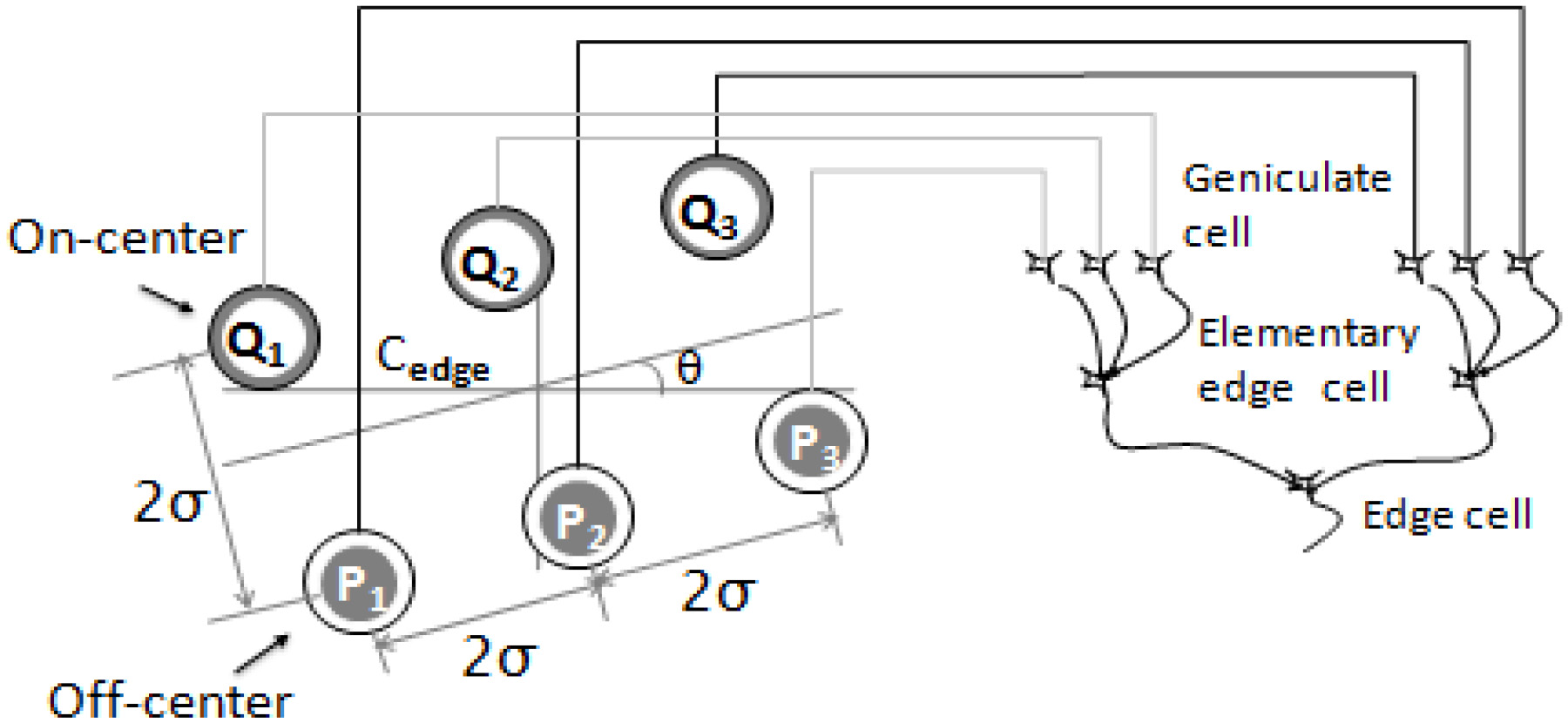
Wiring diagram of an edge cell. A hierarchical structure was introduced by Hubel and Wiesel in order to explain how cortical receptive fields are built up; this hierarchy is made up of simple cells, complex cells and hyper complex cells. Elementary units are used to build up receptive fields of simple cells, termed elementary edge cells; these receive projections from three geniculate cells. An edge cell received projections from the two types of elementary edge cell. Cedge and denoted the center position and orientation of the edge cell, respectively. Pi and Qi (i= 1, 2, 3) indicated the center positions of the receptive fields of OFF-center geniculate cells and ON-center ones, respectively.

2.Differential cell

In their early research, Hubel and Wiesel [14] separated cells into simple cells, complex cells and hyper-complex cells, according to the level of cells in the V1 zone. It is widely accepted that Gabor filters [15], DOG filters [16], Gaussian filters [17], and edge cell [18] research paved the way for the simple cell model. This paper uses the edge cell in a simple cell model that is able to interpret the relationship between the lateral geniculate nucleus (LGN) with the least parameters. The model in Fig. 1 is called “edge cell”. It is adapted from Marr and Hildreth’s model by removing the “logical and gates” parameter. Compared to the traditional models (such as Gabor filter, DOG filter, and Marr & Hildreth), our “edge cell” model placed no restrictions on the size of the simple cell’s receptive field, especially the major axis. The experiment results presented in this paper show that both the size and the separation of geniculate cell’s receptive field were crucial in extracting the features of the contour line. Therefore, it was necessary to establish a base parameter σ based on the size of the simple cell’s receptive field [19]. The response function of the edge cells was defined as follows:

Here ∇2⁡G(X) indicates the laplacian-gaussian value in the X-axis location.

In Fig. 2, if the edge cell (base) was located on the linear edge, and the optimal orientation of the cells coincided with the edge’s orientation, the edge cell would output a maximum reaction value [20]. At the same time, if there was another edge cell (shift) located at regular intervals in the extended line of the edge orientation, and if the response value of the edge cell (base) was less than that of the edge cell (shift), the result would be near zero. If the edge cell (base) was on the curve edge and its center position was verging on the point of contact, the reaction value would be close to the highest value possible. Meanwhile, compared with the reaction value on the linear edge position, the value of the edge cell (shift) would decrease in the extended line of the edge. In that case, the difference in reaction value between the edge cell (base) and the edge cell (shift) would be a positive number. Moreover, this positive number would vary with any change in curvature.

Figure 2.

The edge cell’s two receptive fields on the radian edge that was altered. The receptive field is represented with a rectangle profile. The reaction value of cell E was less influenced by the degree of edge bending, whereas the reaction value of cell I shows a tendency of decrease with an increase in curvature.

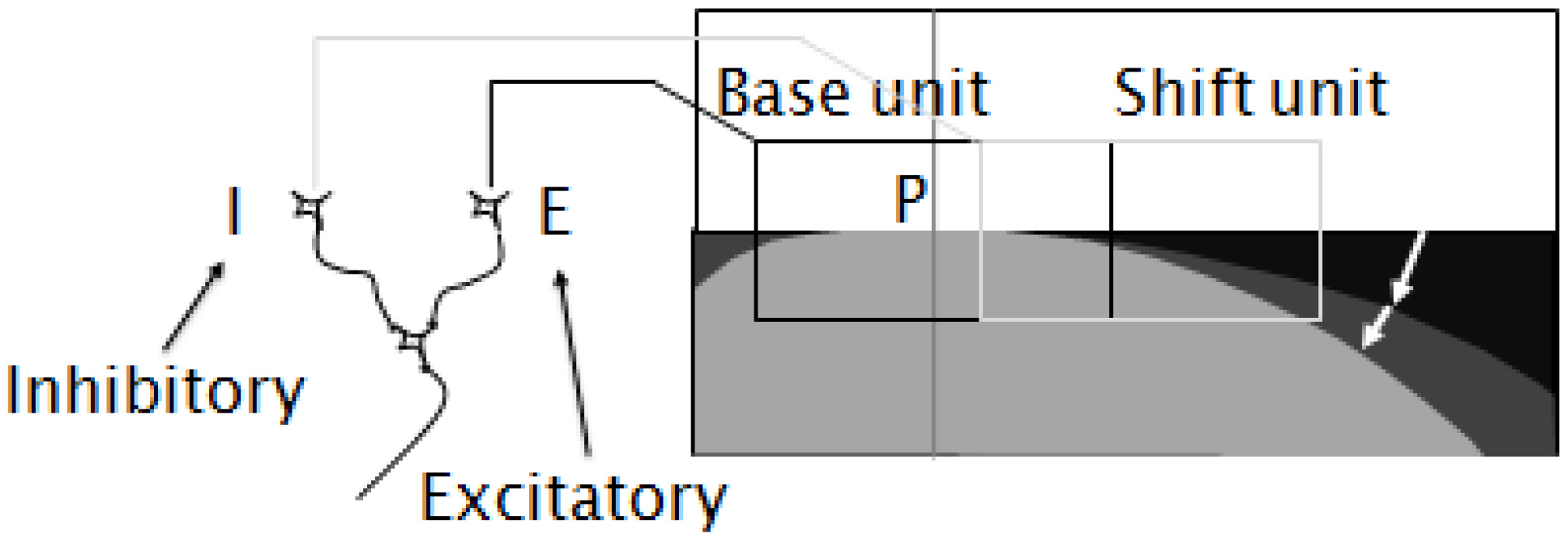
In Fig. 2, when the simple cell’s receptive fields E and I (“E” for excitatory and “I” for inhibitory) are located near the curve tangent line, the cell accepted the difference in reaction value between E and I and could therefore be defined as “differential cell” (Fig. 2). The reaction value of “differential cell” (RD) was defined as:

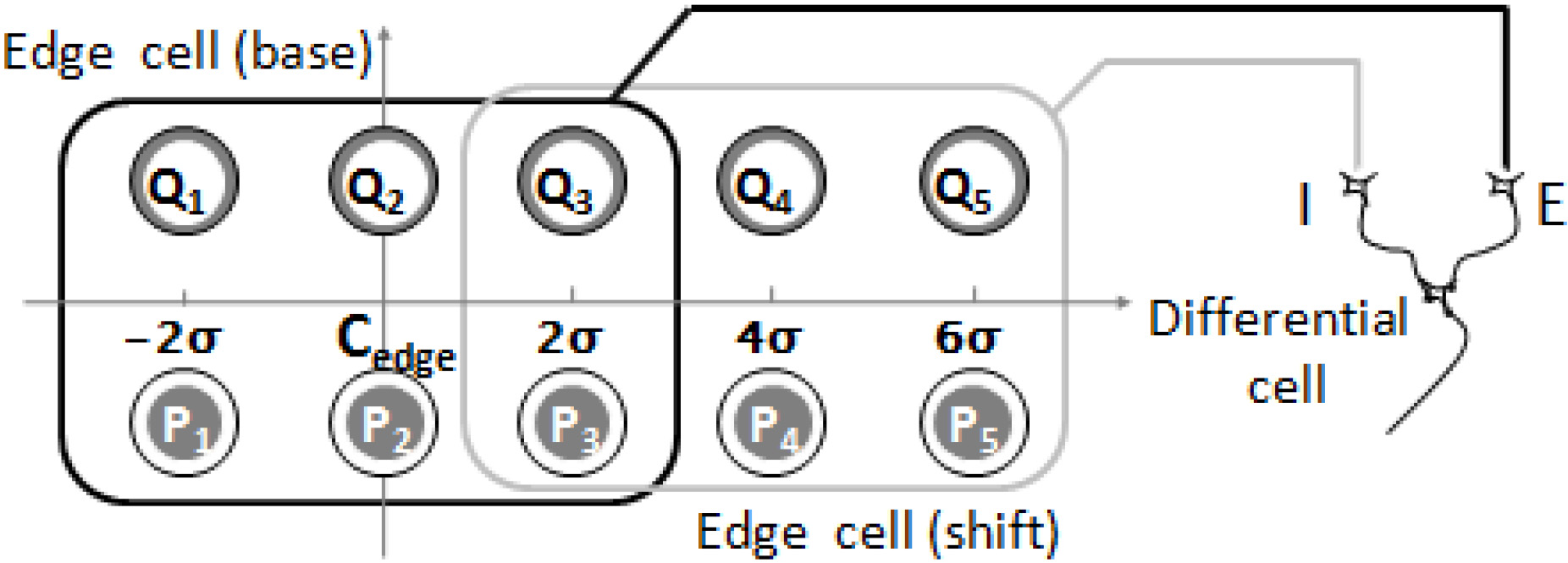
In this formula, REbase represents the the reaction value of the edge cell (base), and REshift represents the reaction value of the edge cell (shift). The differential cell’s receptive field is shown in Fig. 3.

Figure 3.

A schematic model of the receptive field of a differential cell. A differential cell receives projections from two-edge cells, one excitatory (E), the other inhibitory (I). The excitatory edge cell has its receptive field in the region indicated by the left rectangle; the inhibitory cell has its field in the area indicated by the right rectangle.

3.Using the curvature cell to implement curvature detection

In the present study’s definition of “differential cell”, the reaction value was determined by subtracting the value of the edge cell (base) and of the edge cell (shift). This is essentially the same as assuming the existence of a kind of cell that contains both excitatory and inhibitory zones in its receptive field. For example, if the two zones are stimulated simultaneously (for instance, with linear stimulus), the resulting reaction value of differential cell is 0. This is similar to the end-stopped cell’s reaction. The structure in Fig. 3 was called “right-differential cell” (or RDC). If the edge cell (shift) switched positions to the left side of the edge cell (base), it would form another type of differential cell: “left-differential cell” (or LDC). Furthermore, the cell that stimulated by RDC and LDC was named the “curvature cell” (Fig. 4a). The curvature cell could be treated as a specific model of end-stopped cell, where the two ends of the cell were inhibitory in the V1 zone.

Figure 4.

A schematic model of the receptive field of a curvature cell and its response to curved edges. (a) There are two types of differential cells according to locations of inhibitory regions. The curvature cell receives projections from both RDC and LDC (where RDC indicates a differential cell with its inhibition region on the right-hand side, and LDC a differential cell with its inhibition region on the left-hand side). (b) Response of the curvature cell to curved edges. When the radius of curvature is r, the modified curvature is equal to α/r.

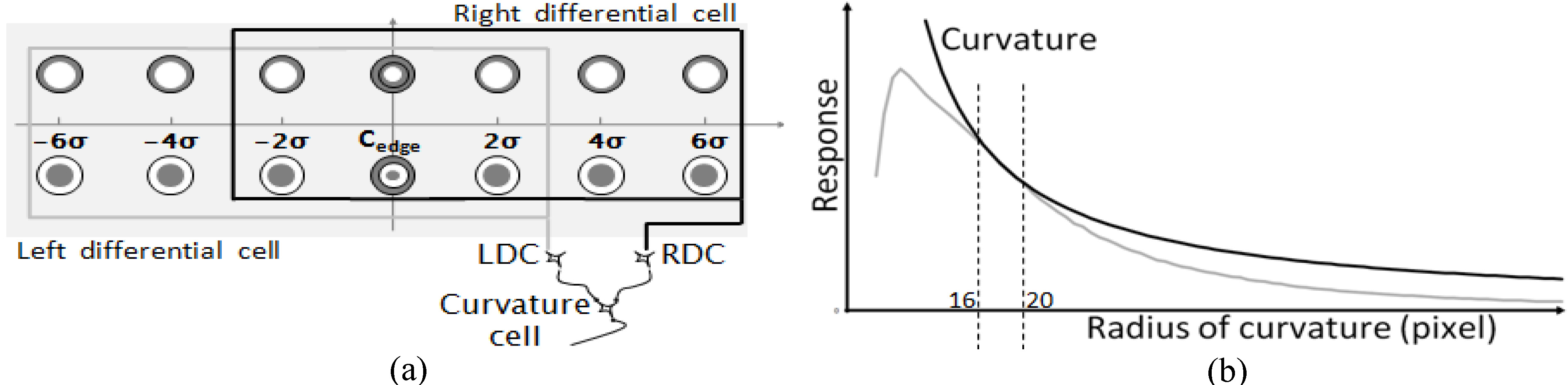
To verify the reaction characteristics of bending of both RDC and LDC, RDC’s and LDC’s reaction values with shifts in radius at a contact position (arc point) were recorded. The curve resulting from their average reaction values was then compared against the corresponding curvature. Figure 4b illustrates the results. When the radius increased, the reaction values’ curve showed a sharp rise followed by a slow decrease. As Dobbins noted in his earlier work, the curve presented a peak value reaction to regions with smaller radius. Although it was possible to distinguish between the curve and the straight line depending on where the reaction’s peak value appeared, the peak value did not allow for accurate measurements of the curvature.

Interestingly, we found that if the reaction value was multiplied by any given number, the reaction value curves and the curvature showed an overlap on a radius of 16–22 pixel drop interval. In certain of these overlap intervals, the decreasing section of the reaction value’s curve was proportional to the change in curvature.

4.Detection of broad range of curvatures

Even though there was an overlap between the two curves (the differential cell’s reaction value and the curvature), two important questions remained: (1) What range of curvature cell could be used for reliable curvature detection? and (2) How to adapt this to a wide range of curvature and response values? In Fig. 4b, after integrating the reaction value curves and the curvature, it is shown that the overlaps happened within a certain range, and so a corresponding relationship between them could also be established. Meanwhile, Fig. 4b also shows that the overlap intervals were relatively narrow, and could only correspond to the arc on a radius of 16–22 pixel. This kind of overlap interval is unable to meet the needs or simulate a visual system bending cognitively in nature. To solve this problem, we introduced a spatial parameter σ, determined on the basis of Wilson et al.’s experiments. For the vision system, Wilson & Bergen proposed a model composed of four different frequencies, and used two Gauss functions (DOG) to describe the excitatory center profile of each frequency. In this model, there are six spatial-frequency-tuned channels, and their peak sensitivities occur at 0.75, 1.5, 2.8, 4.4, 8 and 16 cycle/deg respectively [21, 22]. According to this theory, we can determine the parameter σ by calculating [23]. In the present research, we defined 6 dimensional curvature cell receptive fields (based on Wilson et al.’s notions). These were named CV1, CV2, CV3, CV4, CV5, and CV6; CV1 having the smallest receptive field dimension among them.

Figure 5.

Detection of broad range of curvatures. (a) Schematic diagram for curvature detection. (b) Normalized response curves of CV1, CV2, CV3 and CV4. (c) Attenuated response curves. The deep black curve shows the selector’s outputs.

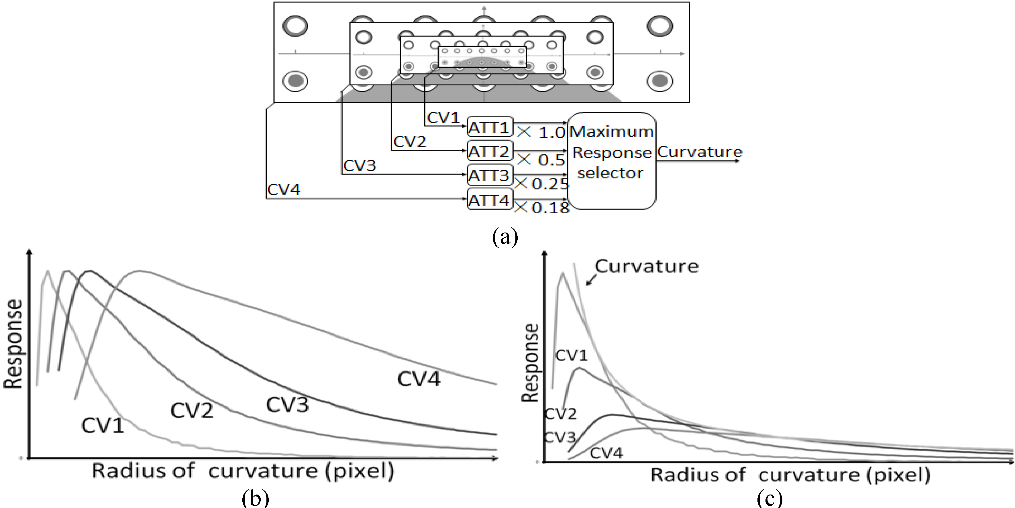
If we could coordinate a variety of curvature cells’ receptive fields to work together and make a selection of their outputs, we could become aware of a broad range of bending [24, 25]. The spatial parameter used here was the empirical value σ1: σ2: σ3: σ4 = 1: 2: 4: 5.7. Figure 5c shows the reactive value curves of four distinct sizes of curvature cells (CV1, CV2, CV3, and CV4), where the corresponding reactive values normalized respectively according to the attenuation ratio of 1: 2: 4: 5.7. The realization of this attenuation relied on the following two considerations:

The results shown in Fig. 5c demonstrate that different resolutions correlated to the change in curvature in different radius intervals. A wider range of curvature was covered by putting CV1, CV2, CV3, and CV4 together. Different ranges of curvature measurements in the visual system were distributed to the corresponding resolution to be processed. The levels of resolution 5 and 6 are not shown in the figure because the corresponding bending radius was too large, and we concluded that the vision system would use alternative methods to identify it.

Figure 6.

The results of curvature detection. (a) The Spiral pattern of gradient of curvature, with radius ranging from 40 to 320 pixels. (b) Contour detection results (spatial-frequency-tuned channels = 4.4 cycle/deg). (c) The response values of differential cells in each position of edge segments. (d) The results of curvature detection in each position of edge segments (CV3 receptive field).

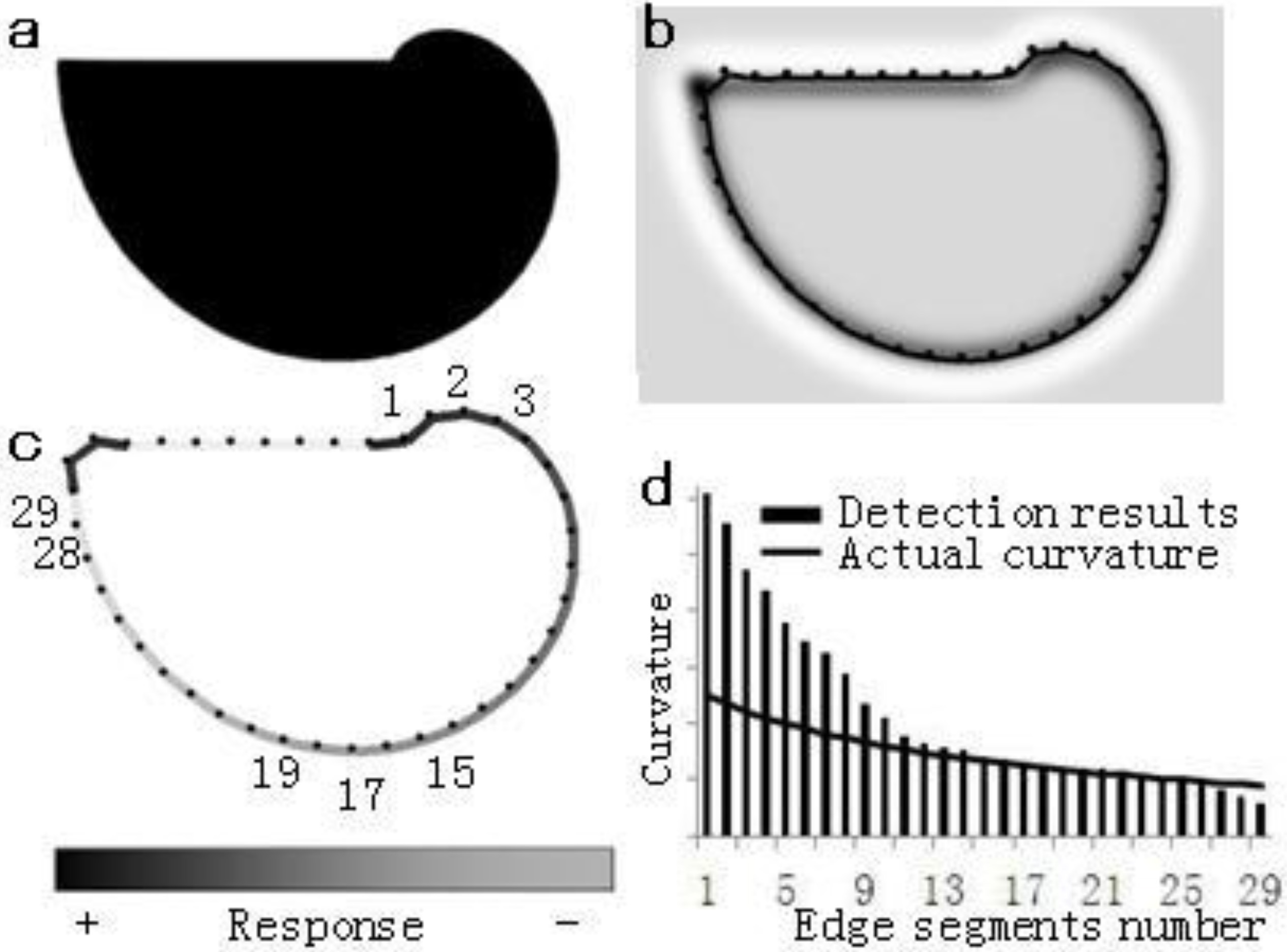
This kind of algorithm still needs to be combined with a contour detection algorithm to fully be able to determine curvature detection. In this paper, a chain algorithm and an edge-cell model are adopted and combined [18]. Figure 6b illustrates the contour detection results of the spiral diagram shown in Fig. 6a. The contour line in Fig. 6b was composed of end-to-end edge segments, with the length of each segment being 4 σ. The differential cells’ response value for each distinct position is expressed as the gray level change shown in Fig. 6c. The results of curvature detection were obtained through calculations dependent on response values. The corresponding results of curvature detection in each position of edge segments were expressed in histogram form. Figure 6d illustrates the detection results of resolution CV3, where the results ranging from number 13 to 25 were almost equal to the actual curvature. This indicates that our method was able to determine the correct curvature detection in the range of a differential cell of the size used. Resolution CV3 corresponded to the radius of the range 145 pixels ∼ 260 pixels; the average error of the detection results was 3.2 pixels. The remainder had to be detected with differential cells of other sizes/dimensions. Meanwhile, the length of the edge segments also shifted with changes in resolution.

Figure 7.

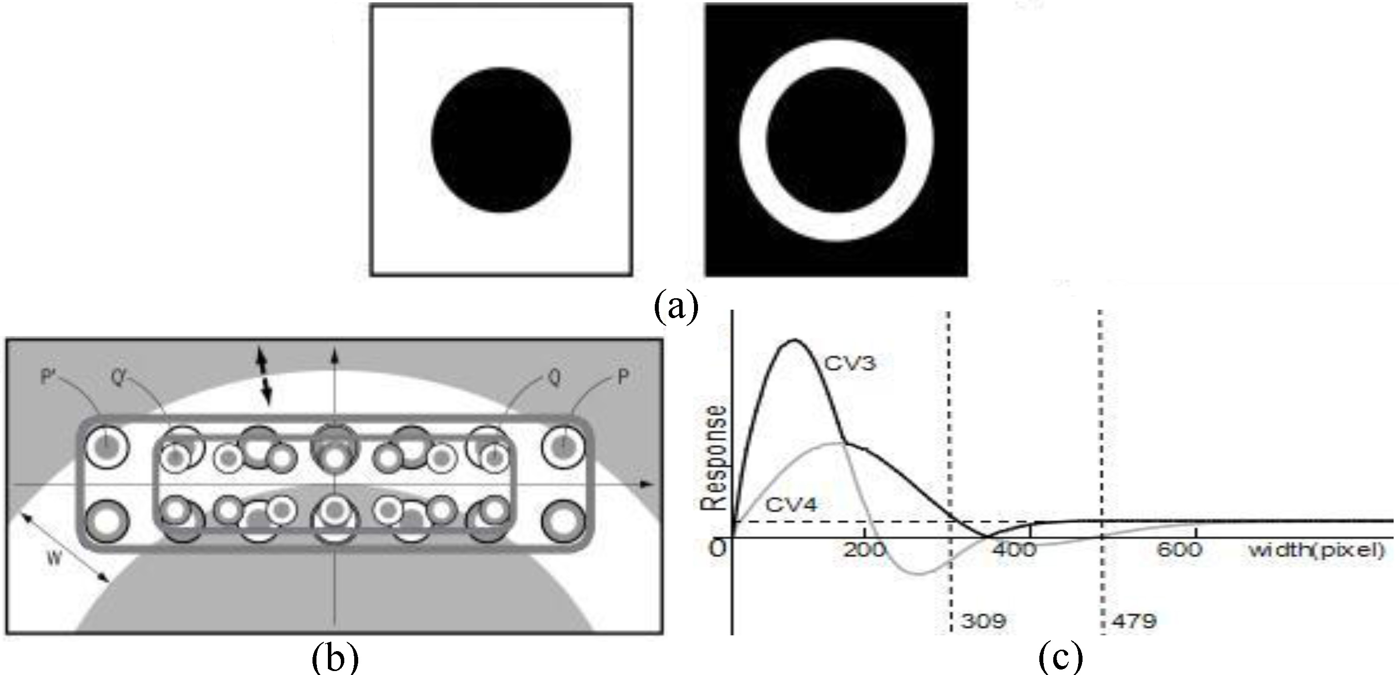
Delboeuf-like illusion. (a) Two black circles of the same size. However, the right circle might be perceived as bigger than the left one. (b) The response curves of the outermost cells P and Q of CV3 and CV4, when there is a dark stimulus on the outside of the black circle. The width W indicates the difference between the radius of the inner circle and the radius of the outer one. (c) The outputs of the maximum response selector in Fig. 3a for a case where the radius of the inner circle is 900 pixels (fixed) and the radius of the outer circle is not fixed. The deep black curve represents the outputs of the maximum response selector.

5.Discussion

To evaluate the validity and usefulness of any vision system theory it must determined whether it has the capacity to accurately explain visual phenomena (for instance, geometrical illusions). The curvature cell proposed in this study could be treated as a projection of eighteen LGN cells (Fig. 4a). When unexpected additional stimuli are added to the receptive field of curvature cells, the cells’ reactive values are impacted, leading to irregular changes and the production of phenomena such as geometrical illusions. In the case study shown in Fig. 7a, the results of a psychology experiment on geometrical illusions illustrated that the black circle on the right looked slightly bigger than the one on the left. The following logic can be drawn from this phenomenon: the visual system selectively chooses curvature cells with appropriate resolutions (e.g., CV3), determined by the size of the target black circle to be recognized. In Fig. 7a with the left black circle the black stimuli appeared on the outermost side of curvature cell’s receptive field. In Fig. 7b, the outermost part of the curvature cell was P and P’ or Q and Q’, and the width of the white ring was 400 pixels. Affected by this, the reactive value of the curvature cell decreased in comparison to the lack of stimulation on the right periphery (confirmed in Fig. 7c). In Fig. 7c, the deep black line represents the reactive value of CV3 and CV4 after ratio attenuation. The horizontal dashed line stands for the reaction value of CV3’s right black circle. It was easily observed that the curvature cell showed a significant reaction to the left side of the figure when the width of the white ring was less than 309 pixels. When the width of the white ring was in the range of 309–479 pixels, the reactive value was lower than on the right side and it clearly showed the over-estimation. With continual decrease of the white ring’s radius, the geometrical illusions gradually disappeared. According to this model’s calculations, the greatest degree of over-estimation was 16%. The Delboeuf concentric-circle illusion demonstrated a similar over-estimation of the size of the inner circle; it was concluded that the Delboeuf illusion might have been caused by the same mechanism.

Many scholars have proposed a variety of neuronal mechanisms for curvature detection. Among earlier research, Dobbins et al. proposed the most promising mechanism: an end-stopping mechanism [1, 26, 27], well-known for being curvature-selective. However, due to ambiguities in responses obtained using Dobbins et al.’s method, this paper proposes that it is more accurate to distinguish the curvature and length of line segments in comparison to curvature detectors [10, 11, 12, 28]. In general, cells in V1 had response ambiguities due to the simplicity and small size of their receptive fields; consequently, the subsequent results could only reflect partial features of contours. These ambiguities in information obtained needed to be transmitted and processed by more complex and/or larger receptive fields. Dobbins et al. proposed a mathematical model of end-stopped cells composed of two simple cells with distinct receptive field sizes. With this research, Dobbins et al. showed that cells exhibiting end-stopping showed selection in the degree of curvature of line stimuli. Since this model contained many parameters, it was difficult to map the response curve to its curvature. This, in part, led to Dobbins et al.’s failure to discover that end-stopped cells signaled the exact values of curvatures.

In other research, Wilson et al. suggested that the visual system contains a multi-resolution mechanism [21, 22]; subsequently, Marr and Hildreth proposed an edge-detection model [19] based on Wilson’s theory. These studies were carried out without considering the multiple scales for straight edges [29]. The questions arose, then, of (1) what kinds of stimuli were suitable for these multiple scales and, (2) how to define the proper scales? In this paper we have showed that four size-specific curvature cells (CV1, CV2, CV3, and CV4) and another two size-specific cells (CV5 and CV6) were required to detect a wider range of curvatures than previously detected (in calculating the size of the cells, Wilson’s empirical data played an essential role). Our model demonstrates how the scale of the cell varies with, and is impacted by, the scale of the stimulus. Both the psychophysical and physiological experiments indicated that the human visual system contained two selective mechanisms for curvature, one for high and the other for low curvatures [30]. The mechanisms of CV1, CV2, CV3, and CV4 corresponded to the former (high curvatures), and the mechanisms of CV5 and CV6 corresponded to the latter (low curvatures).

6.Conclusion

This paper proposes a model that can be used to calculate the response value of differential cells under different curvatures by using images of objects in various resolutions. This model also establishes a differential cell operator, thereby proposing a curvature-based computer system. Use of this mechanism can solve many real-life visual phenomena and correct inaccurate assumptions, such as with the Delboeuf findings.

Conflict of interest

None to report.

References

[1] | Dobbins A, Zucker SW, Cynader MS. Endstopped neurons in the visual cortex as a substrate for calculating curvature. Nature. (1987) . |
[2] | Fan X, Wei H. Research Based on Early Vision Algor Ithm Model. Computer Applications and Software. (2007) ; Vol.24: : p1415.. |
[3] | Lang B, Huang J, Wei H. An image local feature representatin method using hierarchical vision network model. Journal of Computer-Aided Desjgn & Computer Graphics. (2015) ; Vol. 27: : p. 703712. |
[4] | Kato H, Bishop PO, Orban GA. Hypercomplex and simple/complex cell classifications in cat striate cortex. J. Neurophysiol. (1978) ; 41: (5). |
[5] | Orban GA. Higher order visual processing in macaque extrastriate cortex. Physoil Rev. (2008) ; 8: (1). |
[6] | Bolz J, Gilbert CD. Generation of end-inhibition in the visual cortex via interlaminar connections. Nature. (1986) ; p. 362365. |
[7] | DeAngelis GC, Freeman RD, Ohzawa I. Length and width tuning of neurons in the cat’s primary visual cortex. J. Neurophysiol. (1994) ; p. 347374. |
[8] | Sceniak MP, Hawken MJ, Shapley R. Visual spatial characterization of macaque V1 neurons. J. Neurophysiol. (2001) ; p. 18731887. |
[9] | Wilson HR. Discrimination of contour curvature: data and theory. J. Opt. Soc. Am. A. (1985) ; p. 11911199. |
[10] | Wilson HR, Richards WA. Mechanisms of contour curvature discrimination. J. Opt. Soc. Am. A. (1989) ; p. 106115. |
[11] | Gheorghiu E, Kingdom FA. Spatial properties of curvature-encoding mechanisms revealed through the shape-frequency and shape-amplitude after-effects. Vision Res. (2008) ; p. 11071124. |
[12] | Poirier FJAM, Wilson HR. A biologically plausible model of human radial frequency perception. Vision Research. (2006) ; p. 24432455. |
[13] | Gheorghiu E, Kingdom FA. Multiplication in curvature processing. J. Vision. (2009) ; p. 117. |
[14] | Hubel DH, Wiesel TN. Receptive fields and functional architecture in two nonstriate visual areas (18 and 19) of the cat. J. Neurophysiol. (1965) ; p. 29289. |
[15] | Lee TS. Image Representation Using 2D Gabor Wavelets. in Trans. Pattern Anal. Machine Intell. IEEE. (1996) ; vol. 18: : p. 959971. |
[16] | Daugman. Uncertainty relation for resolution in space, spatial frequency, and orientation optimized by two-dimensional visual cortical filters. J. Opt. Soc. Am, (1985) ; vol.2: : p. 11601169. |
[17] | Mokhtarian F, Khalili N, Yuen P. Estimation of error in curvature computation on multi-scale free-form surfaces. Journal of Computer Vision. (2002) ; p 131149. |
[18] | Yu H, Iitsuma S. Detection of displacement vectors through edge segment detection. IEICE Trans. Inf. Syst. (2008) ; p. 234242. |
[19] | Marr D, Hildreth E. Theory of Edge Detection. Proc. R. Soc. Lond. B, (1980) ; vol. 207: : p. 187217. |
[20] | Schummers J, Cronin B, Wimmer K, Stimberg M, Martin R, Obermayer K, Koerding K. Mriganka, SurDynamics. of orientation tuning in cat v1; neurons depend on location within layers and orientation maps. Frontiers in neuroscience. (2007) ; vol.1: : p 145159. |
[21] | Wilson HR, Bergen JR. A four mechanism model for threshold spatial vision. Vision Research. (1979) ; p. 1932. |
[22] | Wilson HR, Macfarlane DK, Phillips GC. Spatial frequency tuning of orientation selective units estimated by oblique masking. Vision Research. (1983) ; p. 873882. |
[23] | Yu H, Niitsuma S. Computational model for calculating curvatures. Trans. Jpn. Soc. Artif. Intell. (2007) ; p. 595603. |
[24] | Briggs F, Usrey WM. A fast, reciprocal pathway between the lateral geniculate nucleus and visual cortex in the macaque monkey. The Journal of Neuroscience. (2007) ; p. 4315436. |
[25] | Wei H, Wang X, Lai L. Compact Image Representation Model Based on Both nCRF and Reverse Control Mechanisms. IEEE Transactions on Networks. (2012) ; vol. 23: : p150162.. |
[26] | Dobbins A, Zucker SW, Cynader MS. End stopping and curvature. Vision Res. (1989) ; p. 13711387. |
[27] | Shao X, Peng Z. Curvature Estimation Methods and Its Application in Surface Detection. Computer Science and Application. (2015) ; p. 239245. |
[28] | Zetzshe C, Barth E. Fundamental limits of linear filters in the visual processing of two-dimensional signals. Vision Research. (1990) ; p. 11111117. |
[29] | Georgeson MA, Freeman TC. Perceived Location of Bars and Edges in One-dimensional Images: Computational Models and Human Vision. Vision Res. (1997) ; p. 127142. |
[30] | Versavel M, Orban GA, Lagae L. Responses of visual cortical neurons to curved stimuli and chevrons. Vision Research. (1990) ; p. 235248. |