
Measuring the 3D motion space of the human ankle
Abstract
BACKGROUND:
The 3D motion space of the human ankle is an important area of study in medicine. The 3D motion space can provide significant information for establishing more reasonable rehabilitation procedures and standards of ankle injury care.
OBJECTIVE:
This study aims to measure the 3D motion space of the human ankle and to use mathematical methods to quantify it.
METHODS:
A motion capturing system was used to simultaneously capture the 3D coordinates of points marked on the foot, and convert these coordinate values into rotation angles through trigonometric functions and vectors. The mathematical expression of the ankle’s motion space was obtained by screening, arranging, and fitting the converted data.
RESULTS:
The mathematical expression of the 3D motion space of the participants was obtained. We statistically analyzed the data and learned that, in terms of 3D motion space, the right foot is more flexible than the left foot and the female foot is more flexible than the male foot.
CONCLUSIONS:
The adduction and abduction rotation ranges are affected by the plantar flexion or dorsal flexure rotation angles. This relationship can be expressed mathematically, which is significant in the study of the ankle joint.
1.Introduction
Both athletes and non-athletes commonly experience ankle injuries. These injuries occur during sports activities and in everyday life. Most people who experience ankle injuries are able to recover after a series of treatments, but some people never fully recover [1, 2, 3]. Surveys have shown that the incidence rate of ankle injuries is growing. Researchers have been working towards a uniform treatment for many years; however, there is currently no clear standard for ankle rehabilitation [4]. It may be possible to use the ankle’s motion space to establish a rehabilitative standard and a grade of the ankle. The rehabilitative standard and grade of the ankle could then be used to diagnose the patient’s condition at various points in time, and to make timely adjustments to rehabilitative training. Studying the ankle’s motion space is valuable for assuring proper treatment protocols.
In addition to its importance in the medical field, studying the ankle’s motion space contributes to medical robotics research. The growing number of patients with ankle injuries, combined with longer recovery periods and difficulties in assessing treatment outcomes, has led many scientists to look for ways to improve the speed and treatment effects through non-drug treatments. One area of research that has been widely studied recently is ankle-rehabilitative robotics [5, 6, 7]. The mechanism of the human ankle is very complex. Its skeletal shape is uneven and each bone in the ankle is constrained by the other bones. Therefore, the rotational angles of the ankle mutually affect one another. Published research has demonstrated one-dimensional rotation ranges of the human ankle [8, 9, 10]. However, these findings do not provide accurate information for establishing a trajectory for an ankle-rehabilitative robot in three-dimensional space, and the reference values of these findings are limited by their dimensions. The mutual relationships of the rotation angles in different directions must be obtained in order for this information to be of use. A more reasonable and effective trajectory can be planned using the measured data of the ankle’s 3D motion space [11, 12]. In the ankle mechanism, movement in different directions is controlled by different bones, muscles, and ligaments [13, 14]. Injured muscles or ligaments could be detected by medical equipment, and targeted therapy and rehabilitation training could be used to achieve better rehabilitation effects [15, 16].
2.Materials and methods
2.1Measuring instrument
In this study, we used a motion-capturing system (Motive) produced by NaturalPoint, Inc. This system is able to acquire accurate data about the actual motion space of the ankle [17]. As shown in Fig. 2, this system consists of 12 cameras, a supporting camera frame, a computer, a rotary head with three degrees of freedom, special clothing, shoes, and marks. These cameras indirectly capture the 3D coordinates of the marked points on the human foot and feed them back to the computer for continuous recordkeeping.
Figure 1.
Motion capturing system.
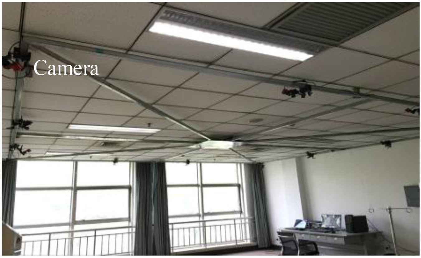
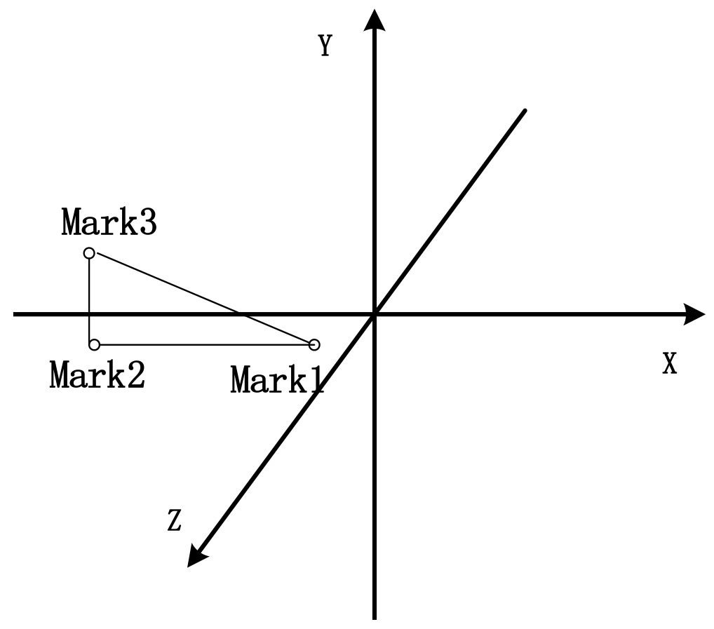
Figure 2.
The coordinate system after calibration.
Sixty graduate students (30 males and 30 females) were recruited to participate in this study. Participant demographic information is shown in Table 1.
Table 1
Participant demographic information (Mean
| Gender | Age | Height (cm) | Weight (kg) |
|---|---|---|---|
| Male | 24.0 | 175.0 | 70 |
| Female | 24.0 | 160 | 50 |
2.2Methodology
The motion capturing system is not able to directly measure rotation angles. Therefore, we used vectors and trigonometric functions to translate the measured three-dimensional coordinates of the marked points into rotation angles in three-dimensional space. In order to follow trigonometric function principles, three markers were needed for data measurement. These markers were named Mark1, Mark2, and Mark3. In order to confirm the relative positions of the cameras in space, and to confirm the horizontal plane, we used the rotary head with three degrees of freedom and the calibration bar to recalibrate the cameras. We did this to avoid any errors that could be caused by slight equipment movements between measurements. Figure 2 depicts the mark positions and the coordinate system that were produced after the calibration of the motion capturing equipment.
If we fixed marks directly on the foot, the data and results would be inaccurate. Some marks might be blocked and the corresponding coordinates would not be able to be obtained through reflection during measurement. Toe movement could also cause measurement errors. We used bandages to horizontally fix a stiff, thin board with three marks on the sole of the foot, through the principle of translation and extension. On the board, the line from Mark1 to Mark2 was perpendicular to the line from Mark2 to Mark3. The positions of the marks are shown in Fig. 4. Using the board prevented metrical errors due to uneven soles, and greatly improved measurement accuracy.
Figure 3.
Mark positions on the board.
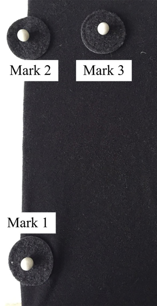
Figure 4.
The measurement process.
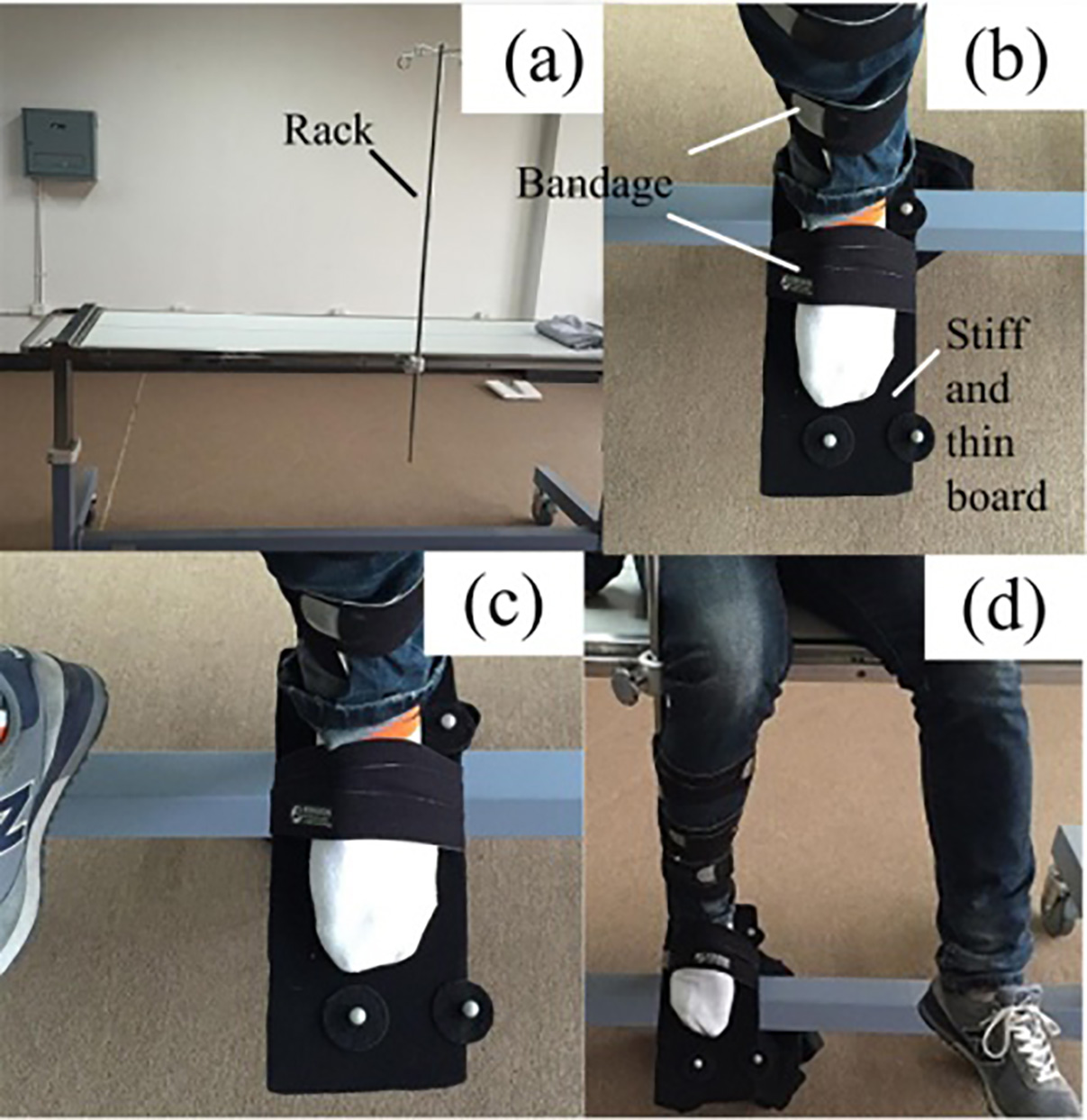
Rotation of the leg following ankle movements can generate falsely inflated data. To address this, a medical bed with an adjustable rack was used during the measurement process. The rack could move both horizontally and vertically. We fixed the rack on the middle of the bed. The leg was fixed on the rack with bandages in order to prevent it from rotating after ankle movement, and the rack was adjusted to an appropriate position relative to the subject’s height to ensure that the rack did not influence the data. This method helped us to obtain more accurate data of the ankle’s 3D motion space. Since the rotation angle is a relative value, we defined a reference point (referred to as the initial state) in which the subject’s leg was perpendicular to the ground, the horizontal plane for the sole of foot was perpendicular to leg, and the toes were in front of the ankle (see Fig. 4b). In this state, the rotation angles of the ankle in all directions were zero. We had the subjects sit on the bed with the stiff, thin board fixed on the sole of the foot while the leg was fixed on the rack in the initial state. Then, a model was built to measure the data. After the equipment started simultaneously recording the mark coordinates, participants let the ankle rotate to reach any point it could achieve in three-dimensional space. After several minutes, we stopped collecting data and recorded the data in a spreadsheet. When measuring the data of the left foot, the participant sat to the left of the rack, as this made it easier for the left foot to be in its initial state, resulting in more accurate data. Likewise, when measuring the data of the right foot, the subjects sat to the right of the rack. The measurement process is shown in Fig. 4.
Through data analysis, we calculated the standard deviation (
3.Analysis and arrangement of data
3.1Basic principles of data analysis
The data of the left and the right foot were separated after all subjects were measured. Table 2 shows the data of one foot. Columns C, D, and E in the table represent the coordinates (
Table 2
The collected data
| C | D | E | F | G | H | I | J | K | |
|---|---|---|---|---|---|---|---|---|---|
|
|
|
|
|
|
|
|
|
| |
| 0 | 1.0812 | 0.4755 | 0.838 | 0.4775 | 0.8435 | 0.4774 | |||
| 1 | 1.0812 | 0.4756 | 0.838 | 0.4775 | 0.8435 | 0.4774 | |||
| 2 | 1.0812 | 0.4755 | 0.838 | 0.4776 | 0.8435 | 0.4774 | |||
| 3 | 1.0812 | 0.4755 | 0.838 | 0.4776 | 0.8435 | 0.4775 | |||
| 4 | 1.0812 | 0.4756 | 0.838 | 0.4776 | 0.8435 | 0.4775 | |||
| 5 | 1.0812 | 0.4755 | 0.838 | 0.4776 | 0.8435 | 0.4775 | |||
| 6 | 1.0811 | 0.4755 | 0.838 | 0.4776 | 0.8435 | 0.4775 | |||
| 7 | 1.0811 | 0.4755 | 0.838 | 0.4776 | 0.8435 | 0.4776 | |||
| 8 | 1.0811 | 0.4756 | 0.8379 | 0.4777 | 0.8435 | 0.4776 | |||
| 9 | 1.0811 | 0.4755 | 0.8379 | 0.4777 | 0.8435 | 0.4776 | |||
| 10 | 1.0811 | 0.4755 | 0.8379 | 0.4777 | 0.8435 | 0.4776 |
3.2Analysis of dorsal flexure and plantar flexion
The rotation angles of the plantar flexion and dorsal flexure were calculated using the Mark1 and Mark2 coordinates. The formula used is as follows:
(1)
If
3.3Analysis of adduction and abduction
Converting the coordinates into rotation angles of adduction or abduction was a complicated process. We had two methods of analysis.
Method I:
We simply used Eq. (2) to convert the data and obtain the results. We had to examine two cases to use this method.
(2)
Analyzing the data of the left foot with the coordinate system led to the conclusion: if
Method II:
We used different formulas to convert the data from the left foot and the right foot. We chose Eq. (2) to convert the left foot data, and Eq. (3) to convert the right foot data.
(3)
When using this method to obtain
3.4Analysis of varus and eversion
There was no difference between converting the coordinates to rotation angles of varus or eversion and the coordinates to the rotation angles of adduction or abduction. We could use the same methods for analysis and conversion. The first formula used is:
(4)
We used Method I to obtain
(5)
The principle of Method II is the same as above. We chose Eq. (4) to convert the coordinates collected from the left feet into rotation angles, and Eq. (5) for the right foot data. If
3.5Initial errors
Table 3 displays the results obtained using Method II in three columns named L, M, and N. The data in the three columns are the three rotation angles that correspond to the position of the foot in the coordinate system, measured in degrees. There were small initial errors because the sole was uneven when the ankle was in the initial state with a hard board fixed on the sole of the foot. We obtained more accurate results using rotation angles that were obtained by subtracting the rotation angles that corresponded to the initial position.
Table 3
The converted data
| C | D | E | F | G | H | I | J | K | L | M | N |
|---|---|---|---|---|---|---|---|---|---|---|---|
|
|
|
|
|
|
|
|
|
| È | â |
|
| 1.081 | 0.476 | 0.838 | 0.478 | 0.844 | 0.477 | 0.461 | 5.904 | ||||
| 1.081 | 0.476 | 0.838 | 0.478 | 0.844 | 0.477 | 0.463 | 5.905 | ||||
| 1.081 | 0.476 | 0.838 | 0.478 | 0.844 | 0.477 | 0.474 | 5.894 | ||||
| 1.081 | 0.476 | 0.838 | 0.478 | 0.844 | 0.478 | 0.479 | 5.903 | ||||
| 1.081 | 0.476 | 0.838 | 0.478 | 0.844 | 0.478 | 0.473 | 5.912 | ||||
| 1.081 | 0.476 | 0.838 | 0.478 | 0.844 | 0.478 | 0.489 | 5.907 | ||||
| 1.081 | 0.476 | 0.838 | 0.478 | 0.844 | 0.478 | 0.491 | 5.922 | ||||
| 1.081 | 0.476 | 0.838 | 0.478 | 0.844 | 0.478 | 0.494 | 5.939 | ||||
| 1.081 | 0.476 | 0.838 | 0.478 | 0.844 | 0.478 | 0.495 | 5.949 | ||||
| 1.081 | 0.476 | 0.838 | 0.478 | 0.844 | 0.478 | 0.511 | 5.951 |
3.6Arrangement of data
Throughout this process, we were working to obtain the 3D motion space of the ankle. This refers to the rotation ranges in various directions at different rotation angles of the dorsal flexure or plantar flexion. Therefore, it was necessary to analyze the data of the points on the edge of the motion space. There were some points that were not on the edge or repeated because the ankle rotated to reach any point it could achieve in the three-dimensional space for several minutes during measurement. We are able to create a preliminary screening from these data. Firstly, the data for the points that were not on the edge were deleted, and then we calculated the averages of the data of the points that could be considered repetitions. Table 4 shows that the data in the first 8 columns should be deleted because they are obviously not the data of points on the edge. The data in the last 3 columns represent points that could be considered repetitions, so we obtained the averages of these columns.
Table 4
The preliminary screening data (in degrees)
| è | 19.03 | 19.15 | 19.25 | 19.42 | 19.37 | 19.42 | 19.50 | 19.46 | 19.41 | 19.32 | 19.08 |
| â | 15.33 | 15.69 | 16.07 | 16.34 | 16.82 | 17.27 | 17.74 | 18.16 | 18.55 | 18.97 | 19.31 |
| ä | 13.98 | 14.21 | 14.39 | 14.79 | 14.98 | 15.27 | 15.42 | 15.71 | 15.85 | 16.26 | 16.54 |
After all of the data were screened the first time, we integrated the data for the left foot into one table and the data for the right foot into another table. We placed the rotation angles for the same direction separately into one column.
When we screened the integrated data the second time, individual data that were significantly different from the others were deleted, and then we calculated the averages of the remaining data. For each number in the first column, there is a corresponding positive number, representing the rotation angle in one direction, and a negative number, representing the rotation angle in the opposite direction. We separately average all the positive numbers and the negative numbers. Whichever average has a greater absolute value, it is used to represent the actual rotation angle.
The final data that corresponded to the motion space of the left foot or the right foot were obtained after the data’s arrangement was completed again. These data are shown in Table 5.
Table 5
Second screening data (in degrees)
| Right ankle data | Left ankle data | ||||||||||
|---|---|---|---|---|---|---|---|---|---|---|---|
| È | â | ä | È | â | ä | ||||||
| | .5 | | .5 | 4 | .4 | | .5 | | | .5 | |
| .5 | 6 | .1 | .7 | .5 | 8 | 2 | .4 | ||||
| .5 | .5 | .5 | .6 | ||||||||
| .5 | 8 | .5 | 5 | .2 | .5 | 11 | 2 | .3 | |||
| .5 | .5 | 3 | .2 | .7 | |||||||
| .5 | 10 | .7 | 13 | 5 | .1 | ||||||
| .5 | .8 | .5 | .5 | .6 | |||||||
| .5 | 12 | 6 | .3 | .5 | 15 | .6 | 11 | .6 | |||
| .5 | .3 | .5 | .5 | .7 | .4 | ||||||
| .5 | 13 | .8 | .5 | 16 | 6 | .7 | |||||
| .5 | .3 | .5 | |||||||||
| .5 | 14 | 6 | .8 | .5 | 16 | .6 | 12 | .8 | |||
| .5 | .8 | .7 | 18 | 25 | .2 | ||||||
Lastly, we integrated the final data for the left foot and the right foot into one table using the same method, and then we obtained the final data for the ankle’s motion space after the averages were calculated. The results are shown in Table 6.
Table 6
The final data of ankle’s motion space (in degrees)
| Dorsal flexure or plantar flexion | .5 | .5 | .5 | .5 | .5 | .5 | 0 | 5 | .5 | 16 | .5 | 26 | .5 | 34 | .5 | |||||||
|---|---|---|---|---|---|---|---|---|---|---|---|---|---|---|---|---|---|---|---|---|---|---|
| Adduction | 2 | .5 | 11 | 20 | .9 | 24 | 27 | .9 | 28 | .8 | 29 | .5 | 27 | 20 | .9 | 14 | .7 | 3 | .5 | |||
| Abduction | 1 | .5 | 9 | 19 | .3 | 21 | .4 | 23 | .5 | 23 | .9 | 25 | 22 | 16 | .6 | 8 | .4 | 3 |
4.The simulation
Figure. 5a and b show fitted curves of the maximum rotation angles of adduction and abduction, which changed with the rotation angles of the dorsal flexure or plantar flexion. We used MATLAB to obtain the fitted equations and curves using the least square method to fit the final data, represented by dots [18, 19, 20, 21, 22]. In these Figures, the X-axis indicates the rotation angles of the dorsal flexure and plantar flexion. The positive axis indicates the rotation angles of dorsal flexure and the negative axis indicates the rotation angles of plantar flexion. The Y-axis indicates the rotation angles of abduction or adduction. The axes are measured in degrees.
Figure 5.
(a) Change of adduction. (b) Change of abduction.
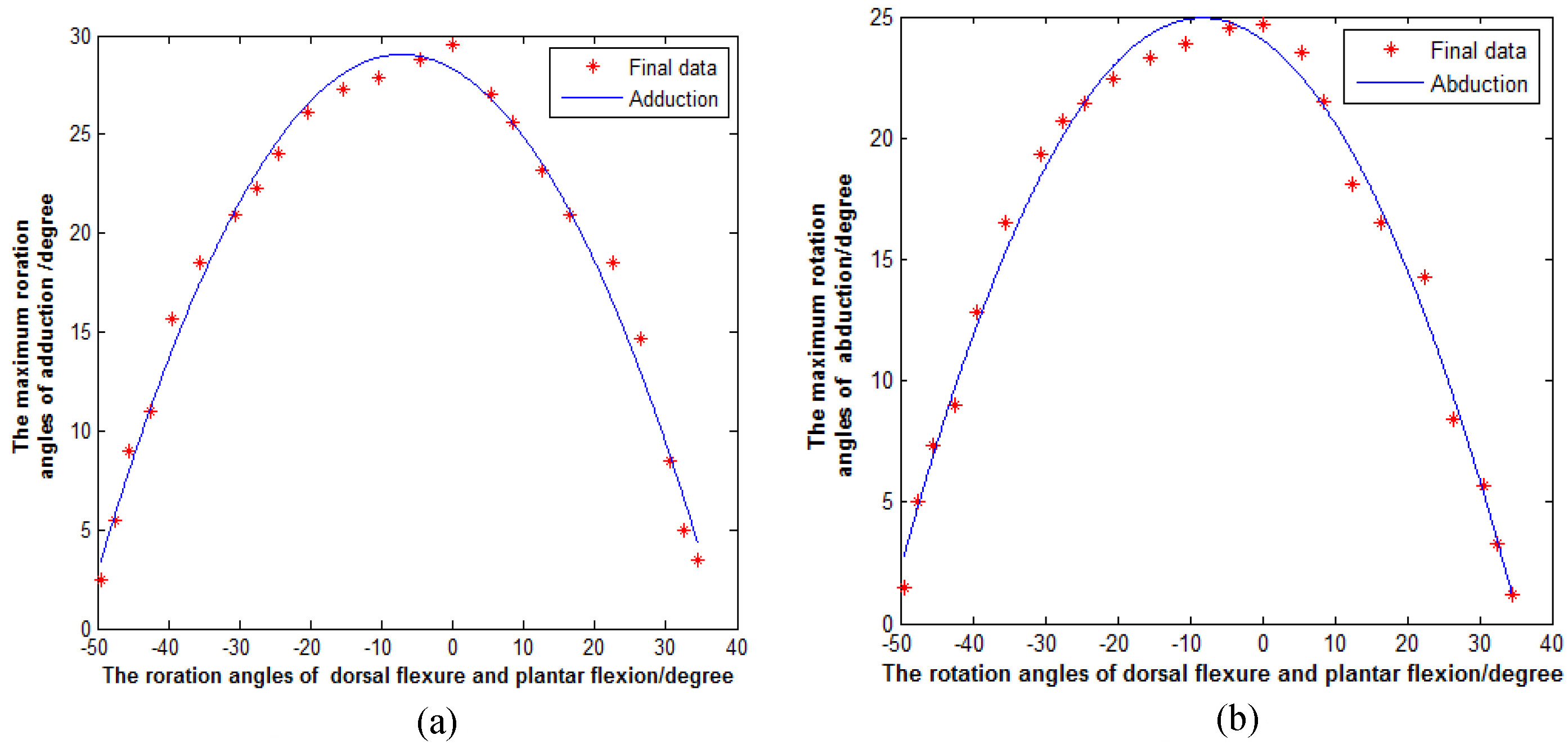
From the graphs, we can see that when the rotation angles of the plantar flexion and dorsal flexure decrease, the maximum rotation angles of adduction and abduction increase. When the rotation angles of the plantar flexion and dorsal flexure are zero, the maximum rotation angle of adduction is 29.5
The maximum rotation angles of adduction and abduction were compared with the same rotation angles for dorsal flexure and plantar flexion. In Fig. 7, the solid curve and dotted line respectively describe the change of the maximum rotation angles for adduction and abduction with the different rotation angles of plantar flexion or dorsal flexure. We also used a
Figure 6.
Comparison of adduction and abduction.
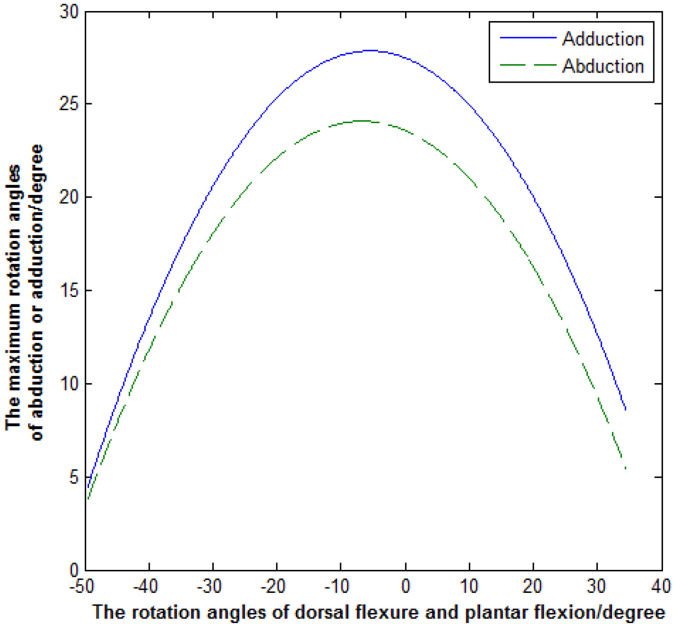
Figure 7.
Three-dimensional graph.
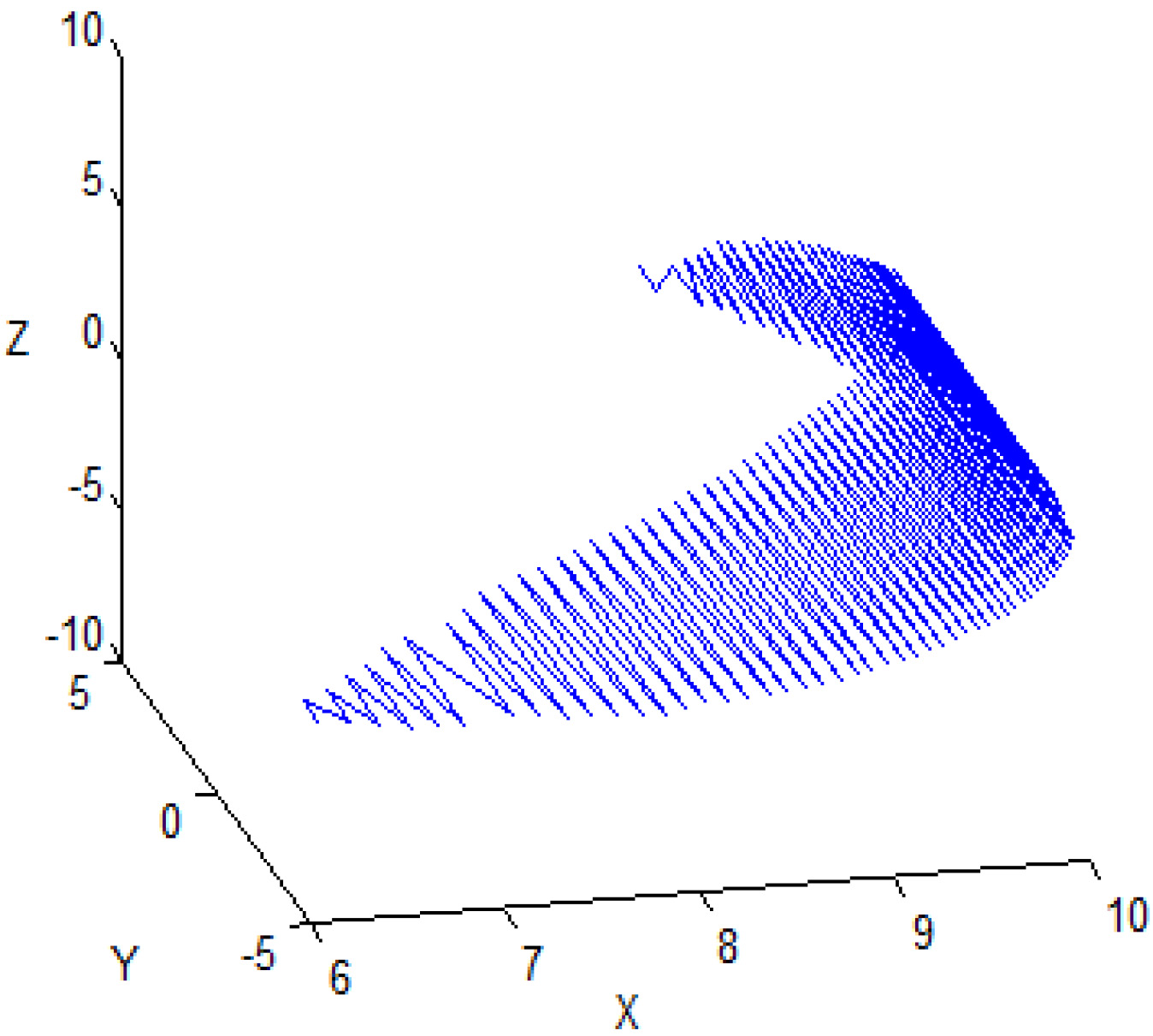
In order to ensure a clear understanding of the ankle’s 3D motion space, we regarded the ankle joint as the origin, and used a particle ten centimeters ahead of the origin to replace the foot. The motion space of the ankle was represented by particles that were obtained by entering the final data into a program that controlled particle movement. The 3D graph of the motion space is shown in Fig. 7. Points on the motion space and the origin form a line. The angle between the line and the plane that is composed of the X-axis and the Y-axis represents the rotation angle of plantar flexion or dorsal flexure; the angle between the line and the plane of the X-axis and the Z-axis represents the rotation angle of adduction or abduction.
5.Discussion
Table 6 shows that the maximum rotation angle of plantar flexion is 49.5
Table 7
One-dimensional rotation ranges of the human ankle
| Directions | Dorsal flexure | Plantar flexion | Abduction | Adduction | Eversion | Varus |
|---|---|---|---|---|---|---|
| Rotation range | 25 | 35 | 15 | 20 | 15 | 25 |
Figure 8.
(a) Change of adduction. (b) Change of abduction.
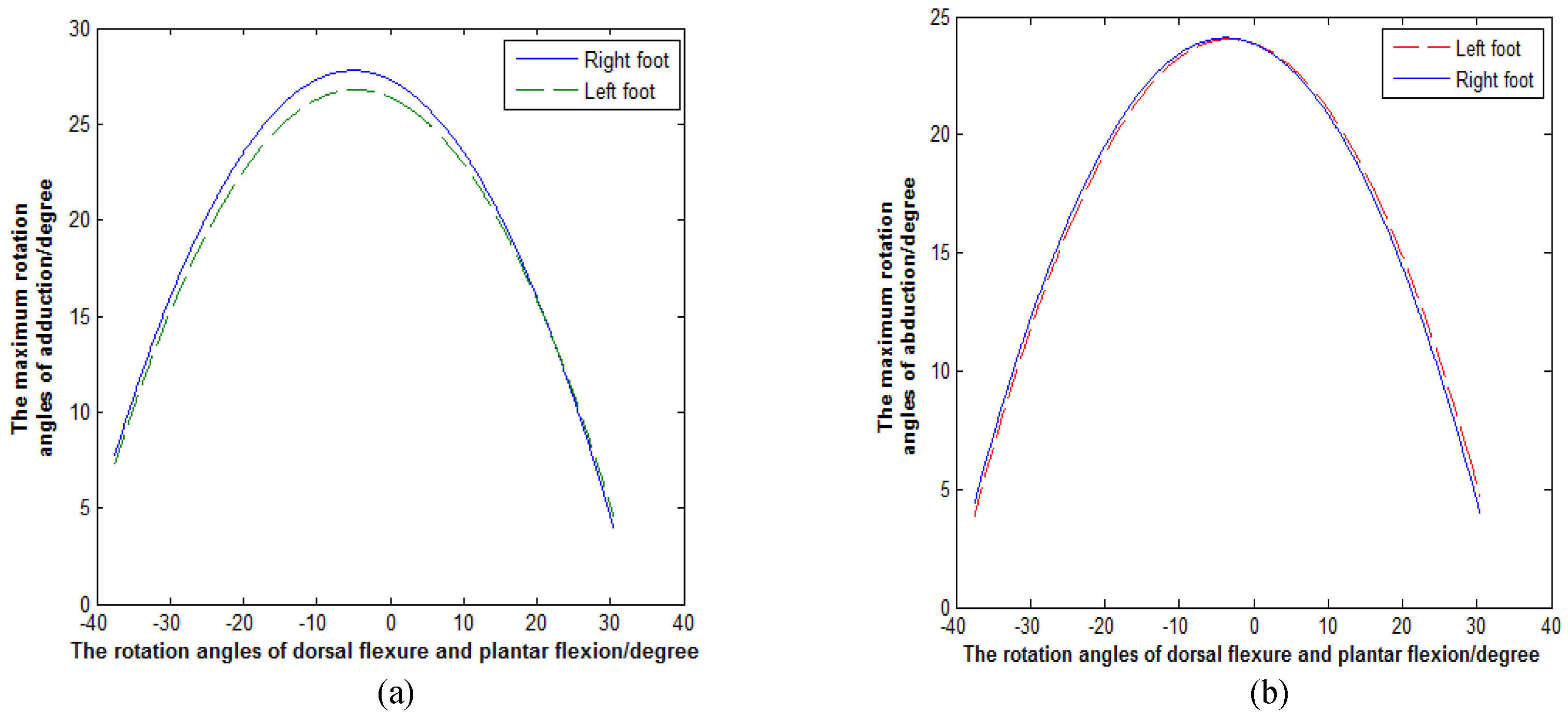
Our experiment used MATLAB to simulate the final data of the left and right feet individually in order to obtain the differences for the maximum rotation angles of adduction and abduction with the different rotation angles of plantar flexion or dorsal flexure. In Fig. 8a and b, the solid curves show the change of the maximum rotation angles for adduction and abduction in the right ankle along with different plantar flexion and dorsal flexure rotation angles. The dotted lines describe the change of the maximum rotation angles for adduction and abduction in the left ankle along with the different plantar flexion or dorsal flexure rotation angles. These graphs show that the motion space of the right foot is slightly larger than the left foot. (The sig of abduction is 0.052, and the sig of adduction is 0.002.). The result shows that the left foot and right foot of subject affect the size of the ankle’s 3D motion space.
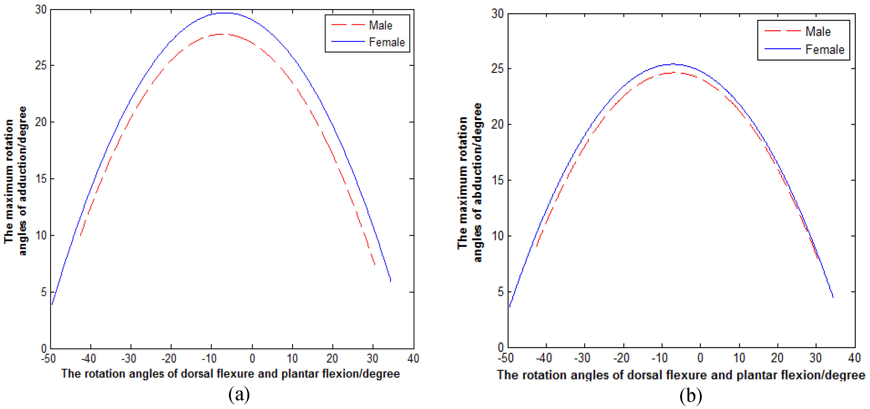
Subject’s age and gender may affect the size of the ankle’s 3D motion space [23]. It should be noted that the results we obtained are slightly larger than the data in Table 7, which may be due to the subjects in this study are young. We used the same method to compare the data of the female and male participants. The simulated results, divided by gender, are shown in Fig. 9a and b. The solid curves describe the change of the maximum rotation angles for the female subjects’ adduction and abduction with the different rotation angles of plantar flexion or dorsal flexure, and the dotted lines describe the change of the maximum rotation angles of the male subjects’ adduction and abduction with the different rotation angles of plantar flexion or dorsal flexure. By contrasting the curves, we see that the motion space of the females’ ankles is significantly larger than that of the males. This means that the females’ ankles are more flexible than the males’ ankles [24]. (The sig of abduction is 0.003, and the sig of adduction is 0.0002.).
Figure 9.
(a) Change of adduction. (b) Change of abduction.
6.Results
The maximum standard deviation of adduction with the different rotation angles of plantar flexion or dorsal flexure is 2.19
The mathematical expression of the 3D motion space of the participants is as follows:
(6)
where
(7)
where
Through analyzing this data, we found that the female subjects’ rotation range of adduction is 1
7.Conclusion
In this study we found that the rotation ranges of adduction and abduction are affected by the rotation angles of plantar flexion or dorsal flexure. Also, the rotation ranges of plantar flexion or dorsal flexure are affected by the rotation angles of adduction and abduction. This relationship can be expressed mathematically. From this information, we can establish a standard of ankle rehabilitation and determine patient recovery using these accurate mathematical expressions. Future areas of research include studying the effect of age on ankle movement space and how the maximum rotation angles of varus and eversion change with the rotation angles of dorsal flexure or plantar flexion.
Conflict of interest
The authors declare that there is no conflict of interest regarding the publication of this paper.
Acknowledgments
The authors wish to thank all the participants who took part in this study and the grant of Key Laboratory of Digital Medical Engineering of Hebei Province, China.
References
[1] | Chinn L, Hertel J. Rehabilitation of ankle and foot injuries in athletes. Clinics in Sports Medicine. (2010) ; 29: (1): 157-167. |
[2] | Czajka CM, Tran E, Cai AN, DiPreta JA. Ankle sprains and instability. Medical Clinics of North America. (2014) ; 98: (2): 313-29. |
[3] | Zhang M. Prevention, and recovery of ankle joint injury in Basketball Players. Contemporary Sports Technology. (2016) ; 6: (2): 14-16. |
[4] | Rodineau J. Rehabilitation of ankle and foot. La Revue Du Praticien. (1986) ; 36: (7): 329-36. |
[5] | Khalid YM, Gouwanda D, Parasuraman S. A review on the mechanical design elements of ankle rehabilitation robot [J]. Journal of Engineering in Medicine. (2015) ; 229: (6): 452-463. |
[6] | Bian H. A novel 2-RRR/UPRR robot mechanism for ankle rehabilitation and its kinematics [J]. Cnki.robot. 2010: (1): 7-21. |
[7] | Dhaher YY, Francis MJ. Determination of the abduction-adduction axis of rotation at the human knee: helical axis representation [J]. Journal of Orthopaedic Research. (2006) ; 24: (12): 2187-2200. |
[8] | Bell-Jenje T, Olivier B, Wood W, Rogers S. The association between loss of ankle dorsiflexion range of movement, and hip adduction and internal rotation during a step down test [J]. Manual Therapy. (2016) ; 21: : 256-261. |
[9] | Kirby KA. Subtalar joint axis location and rotational equilibrium theory of foot function [J]. J am Podiatr Med Assoc. (2001) ; 91: (9): 465-487. |
[10] | Kitaoka HB, Luo ZP, An KN. Three-dimensional analysis of normal ankle and foot mobility [J]. A m J Sports Med. (1997) ; 25: (2): 238-242. |
[11] | Schröder M, Stüber V, Walendzik E. Establishing an optimal trajectory for calcaneotibial K-wire fixation in emergent treatment of unstable ankle fractures [J]. Technology and Health Care. (2015) ; 23: (2): 215-221. |
[12] | Luximon Y, Cong Y, Luximon A. Effects of heel base size, walking speed, and slope angle on center of pressure trajectory and plantar pressure when wearing high-heeled shoes [J]. Human Movement Science. (2015) ; 41: : 307-319. |
[13] | Feger MA, Donovan L, Hart JM. Lower extremity muscle activation in patients with or without chronic ankle instability during walking [J]. Journal of Athletic Training. (2015) ; 50: (4): 350-357. |
[14] | der Wilk D, Dijkstra PU, Postema K. Effects of ankle foot orthoses on body functions and activities in people with floppy paretic ankle muscles: a systematic review [J]. Clinical Biomechanics. (2015) ; 30: (10): 1009-1025. |
[15] | Deng H, Durfee WK, Nuckley DJ. Physical. Complex Versus Simple Ankle Movement Training in Stroke Using Telerehabilitation: A Randomized Controlled Trial [J]. Physical Therapy. (2012) ; 92: (2): 197-209. |
[16] | Wang Z, Zhang Y, Xia S. 3D human motion simulation and a video analysis system for sports training [J]. Journal of Computer Research and Development. 2005: (2): 344-352. |
[17] | Wen J. Establishment and preliminary application of new digital technology on measuring 3D kinematics of intrinsic foot and ankle joint in vivo [D]. Master’s Degree Thesis of Southern Medical University. (2012) . |
[18] | Pointner H, de Gracia A, Vogel J. Computational efficiency in numerical modeling of high temperature latent heat storage: Comparison of selected software tools based on experimental data [J]. Applied Energy. (2016) ; 161: : 337-348. |
[19] | Sorin MO, Nitulescu M. Hexapod Robot Leg Dynamic Simulation and Experimental Control using Matlab [J]. IFAC Proceedings Volumes. (2012) ; 45: (6): 895-899. |
[20] | Ghasemi M, Amrollahi R. Numerical solution of ideal MHD equilibrium via radial basis functions collocation and moving least squares approximation methods [J]. Engineering Analysis with Boundary Elements. (2016) ; 126-137. |
[21] | Ingarao G, Lorenzo R. A contribution on the optimization strategies based on moving least squares approximation for sheet metal forming design [J]. The International Journal of Advanced Manufacturing Technology. (2013) ; 64: (1): 411-425. |
[22] | Yang Y. Curve fitting based on Matlab and the appliantion [J]. Journal of Shanxi Datong university. (2014) ; 17: (4): 34-36. |
[23] | Rein S, Fabian T, Zwipp H. Influence of age, body mass index and leg dominance on functional ankle stability [J]. Foot & Ankle International. (2010) ; 31: (5): 423-432. |
[24] | Qu S, Luo D. Aging of lower limbs’ movement and muscle characteristics of squat in women [J]. Journal of Beijing Sport University. (2015) ; 30: (6): 1-4. |


