
Unbiased estimation strategies for respondent driven sampling
Abstract
In this paper, we focus on respondent-driven sampling (RDS), which is a valuable survey methodology to estimate the size and the characteristics of hidden or hard-to-measure population groups. The RDS methodology makes it possible to gather information on these populations by exploiting the relationships between their components. However, RDS suffers from the lack of an estimation methodology that is sufficiently robust to accommodate the varying conditions under which it is applied. In this paper, we address the estimation problem of the RDS methodology and, by approaching it as a particular indirect sampling technique, we propose three unbiased estimation methods as possible solutions.
1.Introduction
In this paper, we focus on respondent-driven sampling (RDS), which is a valuable survey methodology for both national and international organisations to estimate the size and characteristics of hidden (e.g., homeless people, undocumented immigrants) or hard-to-measure population groups (e.g., minorities, indigenous people).
The principle of “leaving no one behind” is at the heart of the 2030 Agenda and a key requirement for many Sustainable Development Goals (SDG) indicators is to be available for the most vulnerable and marginalised population groups. Nevertheless, halfway through the implementation of the 2030 Agenda, most SDG indicators are still not available at the needed level of disaggregation to monitor the socioeconomic conditions of hidden and hard-to-count population groups. As a result, it is neither possible to produce reliable structural data on the needed disaggregation dimensions nor to monitor the developments of emerging phenomena that need to be approached with targeted evidence-based policy interventions.
The RDS methodology makes it possible to gather information on these populations by exploiting the relationships between their components. Moreover, the effectiveness of the RDS can be further increased by employing an integrated approach in which the RDS is used in conjunction with other information sources, such as administrative or geographical data.
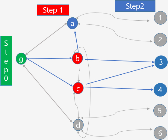
The RDS is a network-based sampling technique [1, 2] that was developed first by Eckathorn [3]. RDS has been the favourite survey method for sampling populations that are difficult to reach due to the potential of a viable sampling technique with reasonable inferential approaches. As a result, since its establishment, it has been employed in countless investigations of these populations across many countries [4]. RDS starts with a small sample of individuals (“seeds”) with which the researchers are familiar. Each participant is then given a small number of coupons with unique identifiers to distribute to their contacts in the target population, enrolling them in the study and growing the sample size until the sample includes the desired number of respondents. The RDS process stops either when, in the selection process, we encounter only units already identified in the previous steps or at a predetermined data-collection step (e.g., the fifth step). Picture 1.1 below illustrates an example of a network sampling process articulated into three steps. The blue lines are the links observed in the sample. Up to and including step 2, participants g, b, c, a, 3, and 4 are kept in the sample. Participants d, 1, 2, 5, and 6 are not observed.
Figure 1.
Example of network sampling process
We may view RDS as a specific extension of the extensively used group of convenience sampling methods known as “snowball sampling networks” [5] which are frequently employed as a last option when a traditional sample frame is not available [6]. Compared to those of more traditional snowball sampling, RDS offers two key benefits. First, respondents receive few coupons. This enables statistical inference to be more appropriately defined and makes it more plausible to approximate the final sample as a probability sample. Second, asking respondents to pass coupons to their contacts in a potentially stigmatised community reduces potential confidentiality issues. Due to this innovation, RDS is a compelling method for gathering data from marginalized and difficult-to-reach populations.
However, the RDS methodology suffers from the lack of an estimation methodology that is sufficiently robust to accommodate the varying conditions under which it is applied. Although it is quite robust for estimating mean and proportion values [7], the accuracy of the total estimates depends on several features including the nature of the network connecting the individuals in the population and the lack of a rigorous sampling approach to select the sampling units.
In this paper, we address the estimation problem and by approaching the RDS methodology as a particular indirect sampling technique [8], we propose three unbiased estimation methods as possible solutions. In particular, the first method assumes a random sampling of the initial individuals. In contrast, the second method, which considers purposive sample selection, creates a nonbiased estimation if the initial sample of respondents falls into all the clusters of networks that characterise the population of interest. Finally, leveraging the generalised capture-recapture estimation approach [9], we propose an estimator that accounts for the noncoverage of two independent indirect samplings.
The paper is organised as follows. In Section 2, we summarise the traditional methodology of the RDS methodology, illustrating the data collection technique and the Volz and Heckathorn estimator [10], which has been very successful in practical applications due to its lack of computational complexity. Section 3 introduces the basic symbology, and we show how the RDS can be seen as a particular specification of indirect sampling in which each survey wave represents the indirect basis for the subsequent RDS phase. In Section 4, we expand the sampling aspects in the RDS. Section 5 introduces the three estimators. Section 6 concludes the work, and we begin to outline a strategy to overcome information gaps for SDG indicators for hard-to-reach populations, focusing on indigenous peoples.
2.Data collection and estimation in the classical RDS approach
RDS is frequently carried out by using techniques suggested by Salganik et al. [11] and outlined in protocols such as those proposed by White et al. [4] and Johnston [12].
A preliminary sample of typically 2 to 10 seeds is chosen. Aiming to represent all the key socioeconomic subpopulations that researchers anticipate may exist in the target population, seeds are selected to be as varied as possible. The rationale of this derives from the fact that each subpopulation may represent a separate network (or a cluster) of target individuals. If we select a seed in a given subpopulation, we can explore the network of related individuals. In contrast, if we do not select any individual in a subpopulation, the specific cluster of individuals cannot be observed in the RDS process. Therefore, picking up in the initial sample all possible distinct networks increases the possibility of constructing unbiased inferences on the target population.
The enumerators should include community opinion leaders in the initial seeds. Hence, their acceptance and support of the survey method may likely inspire widespread involvement from other target population members. This buy-in is crucial in target populations that are unlawful or stigmatised, especially if the population has any prior exposure to risky research practices. Following an interview, the seeds are given some coupons, each with a unique identification number, to spread to other population members. This number was used to reconcile the practical need to prevent the early termination of the sample trees with the inferential aim of limiting the branching of the sample. Members of the population who receive coupons visit a study centre where they are directly interviewed or given an interview appointment. Three coupons are likewise supplied to subsequent replies; this process continues until the sample size is approximately reached and the coupons are tapered or discontinued. Participants are paid for their time spent taking the survey. Additionally, for each successful recruiting, participants receive rewards. In the survey, the number of target population contacts of each respondent must be measured. This is typically done by asking questions that narrow the recruit’s references to the precise definition of the target population. Interviewers must also verify membership in the target population. Researchers must also assure participants do not participate in the survey more than once. Study staff are familiar enough with the target population in many settings to notice repeat participation attempts. In other cases, repetition is prevented by collecting nonidentifiable but unique information about participants, as in Johnston [13].
The RDS methodology can be applied alternatively to the entire population of individuals or by considering only the subpopulation at risk of belonging to the target population. For instance, if the target population coincides with forced labour people, we may observe people working in sugarcane.
Figure 2.
Example of target population divided in disjoint clusters.
Contrary to what was previously believed, Eckathorn [3] used a Markov modelling of the peer recruitment process to demonstrate that bias from the convenience sample of beginning participants from which the sample started gradually diminished as the sample increased wave by wave. By using the model, they demonstrated how the sample approached an equilibrium independent of the beginning location or independent of the convenience sample of seeds from which it started as it expanded wave by wave. The conclusion was that this sampling technique may become reliable if there were enough waves, meaning that any seed selection can eventually yield the same equilibrium sample composition. However, the researchers did not show how an unbiased estimate can be derived.
Eckathorn[14] introduced the first RDS population estimator based on the essential idea that in RDS, relationships tend to be reciprocal. This implies that if person A knows person B, then B knows A.
The estimator bases its validity on the principle of network balance between population subgroups. Up to a constant factor, the volume of network connections to and from each group can be approximated. For each pair of groups, this results in a set of balance equations that may be used to solve for the relative size of each group. Volz and Eckathorn [10] proposed a slightly biased estimator. In the following we call this estimator the VH estimator. The VH estimator is based on the following hypotheses [15]: 1. The network size is large compared to that of the realised sampling, including the initial seeds and the respondents recruited by the RDS process. 2. Homophily is weak enough, where homophily is the tendency for nodes to preferentially form network contacts with others like themselves. 3. Reciprocity of contacts. 4. With-replacement sampling. 5. Enough sample waves. 6. Accurate measurement. 7. The recruitment in the subsequent waves of the RDS process is random.
The first three hypotheses relate to the nature of the contact network, while Hypotheses 4 to 7 relate to sampling. Hypothesis 4 is the most critical and may introduce a certain level of bias, as the sampling process adopted assumes a link between the persons recruited.
Focusing on the first three assumptions, let us consider the example below in Fig. 2, where we assume that people of the target population belong to three disjoint clusters. If the starting sample includes only persons in one group, the traditional RDS can estimate only the total number of persons in that cluster suffering from a substantial undercoverage problem. Since people of the target population are often grouped geographically, observing each cluster’s units in the starting sample is appropriate.
The VH estimator has had great application success in the practice of real investigation due to its great computational ease. Subsequently, other estimators have been proposed in the literature (see among others [16, 17]) each of which overcomes some of the limitations associated with the assumptions made with the VH estimator. These estimators have higher computational complexity, and introduce some modelling assumptions on the cluster variables or the nature of the contact network.
To illustrate the classical VH estimator, let us consider the case where the total of a characteristic
(1)
in the population of interest
Let
The probability of selection of unit
where
where
be the Hansen Hurwitz (HH) [18] estimate of
is the HH estimate ratio of the average number of contacts in the population. The numerator on the right-hand side of the previous equality is given by:
Figure 3.
Example of construction of the totals
The denominator can be expressed as
The VH estimator of
(2)
where
(3)
is the sample weight assigned to unit
3.Totals of interests and a formalisation of the RDS as a particular case of indirect sampling
The RDS can be formalised as an indirect sampling scheme. In this type of sampling, there is an initial
In our case,
The specific unit
(4)
be the value of the characteristic of interest for unit
In the initial population
The two populations
(5)
Moreover, the target parameter may also be expressed as the sum of the
(6)
Indeed, it is
(7)
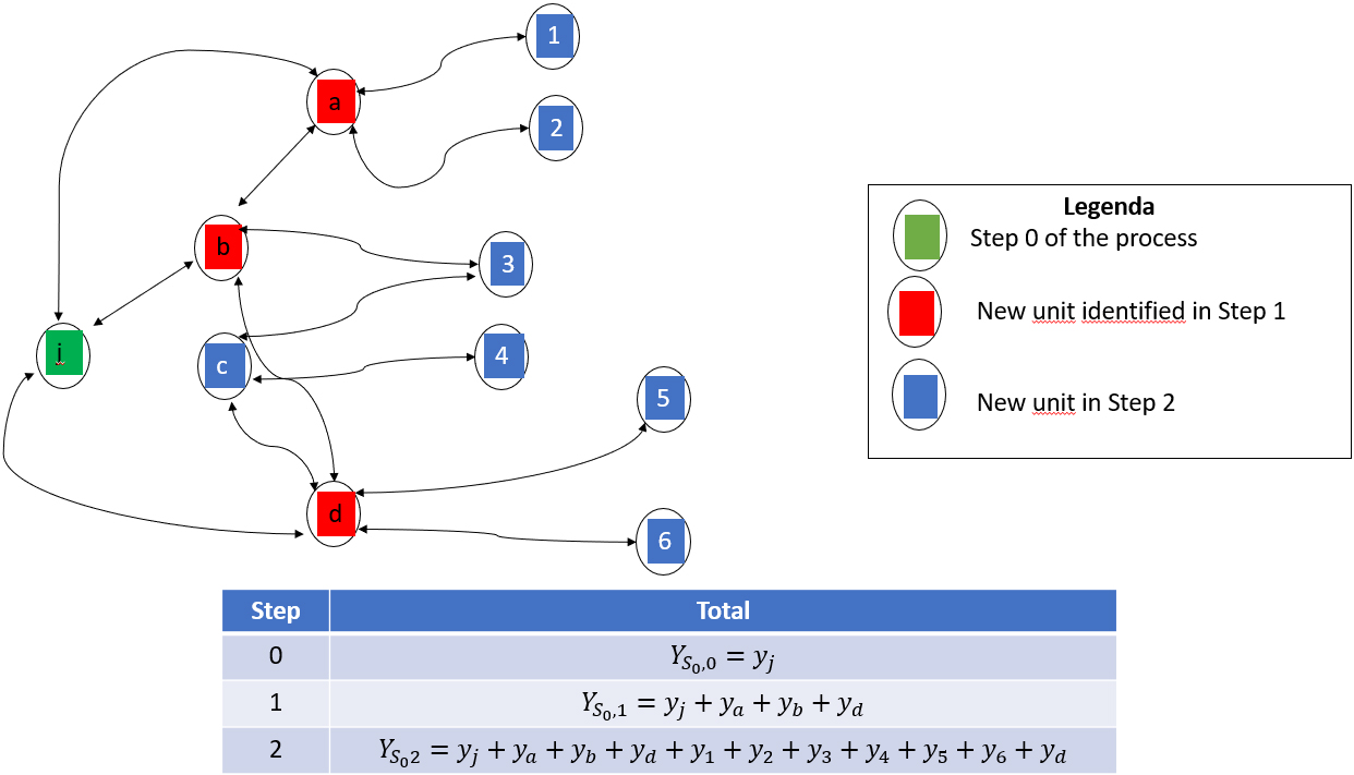
In addition to the total
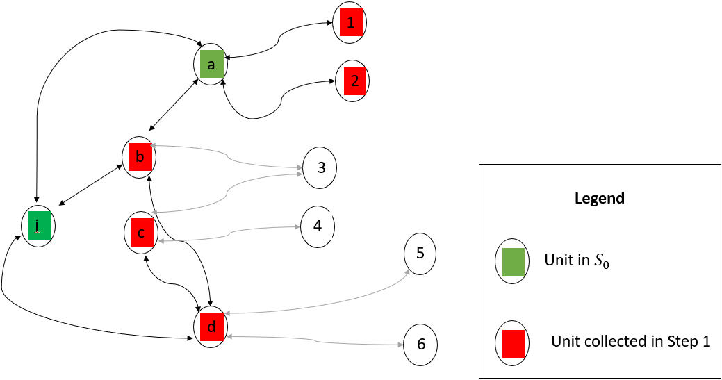
Figure 3 illustrates this process starting from sample
To clarify how this total can be constructed, let us compute it step by step. To distinguish among the search processes of the different steps, let
At step 0, the total
(8)
In step 1, we observe the links of units in
(9)
where
To clarify the notation, we note that the
We can reverse the order of the sums and formulate as
(10)
where
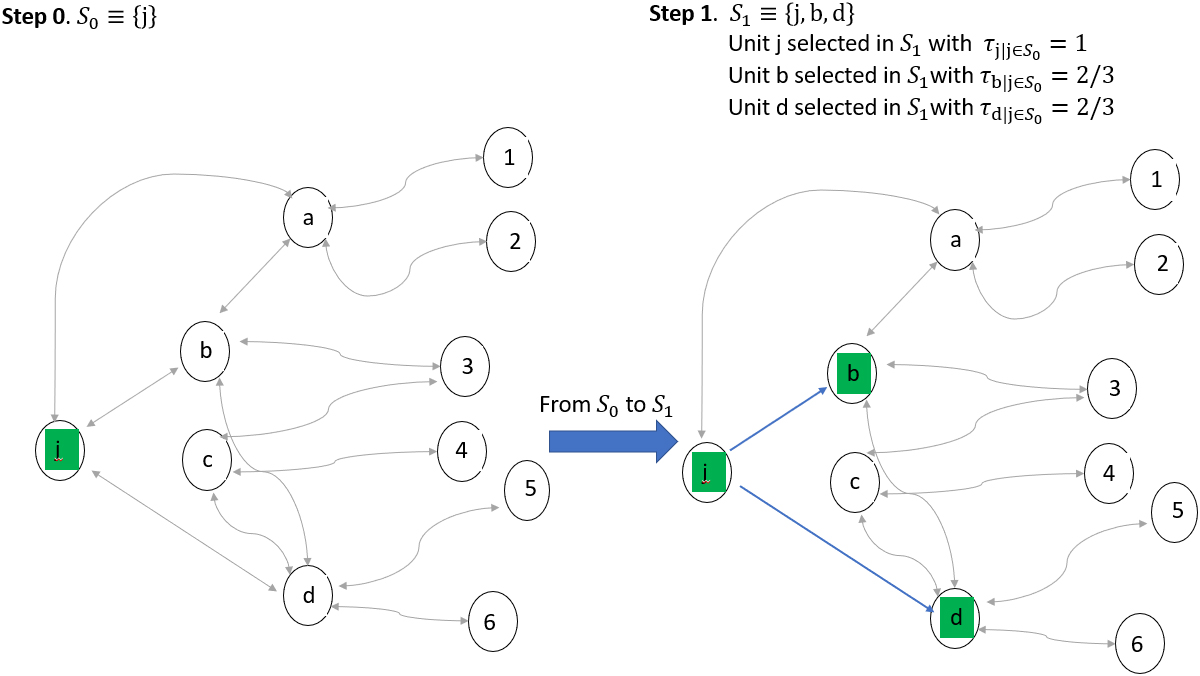
We note that Eq. (10) avoids the multiple counting of a unit linked to different elements of the initial sample, as illustrated in Fig. 4, where unit
Figure 4.
Example of Steps 0 and 1.
At step 2, we have
(11)
We note that the last summation is over
Reversing the order of the summations, we have
(12)
Let us note that in this case, the unit
Continuing recursively the above process, at step
(13)
Even in this case, we avoid the multiple counting of a unit linked to different elements collected in the
Based on the above expressions, we note the following.
• Each step of network sampling can be formalised as an indirect sampling mechanism.
• In a given step of the RDS process, the participants from which the search starts constitute the source list
• In the subsequent step, the people found in the target population
• This switch in the role of the sample participants, from the target population
Remark 1. A path in graph theory is a finite or infinite sequence of edges that joins a sequence of vertices. We note that if
•
• if
We obtain these important outcomes illustrated in remarks 2 and 3 below by interpreting the result of Remark 1 in an alternative way.
Remark 2.
•
• The
Remark 3. We consider the case of two interconnected units in which they know each other. However, these units may belong to two separate clusters if the RDS search rules call for stopping the search if a connection is identified with a person living in a geographic location distinct from that of the original contact. In this case, to ensure the equality
4.Sampling the RDS research chain
Unlike in the previous section, in the RDS process, not all links of a unit kept in the process are observed, but only a randomly selected sample of them is observed. The RDS process starts at step
the total number of contacts of the unit that have been selected in sample
be the number of contacts that have not been selected in sample
Figure 5.
Example of the formation of sample
Remark 4 on the feasibility of the selection process. The illustrated selection process avoids the dead-end loops typical of graph sampling. However, to make it feasible, it is essential to know the
Remark 5 on the research chain for a subpopulation. We consider the case of constructing the RDS sampling search chain only on the units of a subpopulation, for example, only on the people of a particular class-age. We denote by
The values
5.Estimators
Next, we present three estimators. The first assumes a random selection of the
5.1S 0
Let us suppose a random sample
(14)
To facilitate the understanding of the calculation method, we construct the estimator step by step. In each step, we obtain a sampling unbiased estimate of the total
At step 0, we have the classical HT estimator:
(15)
where
In Step 1, we have
(16)
As illustrated in Appendix 2, denoting
(17)
where
Estimator
(18)
where
In Step 2, taking Eqs (16), (17), and (18) of step 1 as a reference, the unbiased estimator
where
and
Recursively using the previous procedure, at the ultimate step
where
and
In Appendix 2, we see
Remark 6 on estimating the sampling variance. We can approximate the RDS design with multistage sampling with replacement, where each step may be viewed as a specific sampling stage, and the replacement refers to a single unit. In that way, we may derive an estimate of the sampling variance [19][(Formula 11.35)];
where
and
Remark 7 on the estimator for a subpopulation. As illustrated in Remark 5, the link variables are defined as
Remark 8 on type of estimator. Considering the above expressions, we can see how the
Remark 9 on the starting sampling. The sampling design should maximise the number of observed individuals of the target population in the sample
5.2S 0
If the sample
where
We note that the formulation of
Remark 10 on type of estimator. We can straightforwardly see how the
Remark 11 on the starting sampling. To ensure that estimator
5.3Generalised capture-recapture estimator
Even if the
Likewise, if the
The generalised capture-recapture (CReG) estimator allows us to overcome the abovementioned undercoverage by leveraging a capture-recapture perspective. A comprehensive treatment of this estimator and how it mitigates undercoverage deserves much more space in this article than can be devoted. The interested reader can undoubtedly look to the extensive work reported in [9].
Let us consider two independent surveys based on the RDS methodology, and we suppose they are articulated in
where
where
A useful approach is applying the estimator CReG on the two nonrandom starting samples but with a different mechanism of undercoverage of the two respondent groups.
6.Conclusions
The disaggregation of data for SDG indicators on hidden or hard-to-count population groups presents several critical issues that are difficult to overcome to produce reliable official statistics at the national and international levels. In this context, it is impossible to estimate the characteristics of these groups through models as in other situations.
Considering, for example, indigenous populations, data availability varies widely from country to country. Few countries provide up-to-date and high-quality data. Many other countries have only data that are scattered over time. Or the data they provide is not supported by a sufficiently robust methodology, both for precisely identifying the subpopulation group of interest and for the sampling technique adopted.
Given the current context of producing official statistics on the subject, it is unrealistic that this lack of data on indigenous peoples is going to improve soon.
Therefore, it becomes necessary to define and apply an implementation program that can improve this situation relatively quickly.
This implementation program should be based on the following pillars:
1. The first pillar is to develop a valuable data collection strategy for sample surveys that is capable of measuring the number of people belonging to the indigenous population in a given area. This strategy needs to cover various aspects, including the formulation of the questionnaire for identifying persons belonging to the indigenous population and the characteristics of special sampling techniques that can maximise the efficiency of surveys aimed at obtaining data on these hidden or hard-to-measure population groups. Specifically, the data collection strategy consists of technical manuals, open software modules, ad hoc training materials, etc. In short, anything that enables or helps conduct surveys or specific survey modules to estimate the size of indigenous populations. Regarding the questionnaire, the data collection strategy should develop a set of standard questions on the key characteristics of the specific population of interest and not adopt generic questions on whether specific individuals belong to an indigenous population group.
2. The second pillar is to adapt the data collection strategy to ongoing survey programs. For example, the indigenous module may be applied to a large-scale national survey conducted by a national statistics office. Another example can be to promote the application of the indigenous sampling module to international surveys, such as the World Bank’s LSMS survey. Regarding the sampling aspects, it is helpful to consider an overall sampling strategy to maximise the number of observed individuals of the target population in the sample by combining the first and final sampling stages. First-stage methods should tend to oversample the areas where the researchers have some a priori information on the geographical concentration of the target population. Final-stage sampling should oversample the target population by adopting strategies, such as respondent-driven sampling (RDS), that leverage the existing hidden relationships among the individuals of the target populations.
3. The third pillar is adopting estimation methods that allow unbiased estimates of phenomena of interest in target populations. In this paper, we have considered the RDS, widely used for observing hidden or rare populations but which lacks an estimation methodology that is sufficiently robust to accommodate the varying conditions under which it is applied. We have proposed three unbiased estimators. The first assumes a random selection of the starting sample, and the second considers a nonprobabilistic starting sample. The third estimator is developed under a capture-recapture approach and allows for smoothing of the coverage problems that may affect the estimators. We have studied their sampling expectation and have indicated the conditions that may be fulfilled to guarantee their unbiasedness concerning the target totals.
References
[1] | Gile K, Beaudry IS. Handcock MS, Miles Q. Methods for Inference from Respondent-Driven Sampling Data. Annu Rev Stat Appl. (2018) ; 5: (4): 1-429. |
[2] | Heckathorn DD, Cameron J. Network Sampling: From Snowball and Multiplicity to Respondent-Driven Sampling. Annual Review of Sociology. August (2017) . |
[3] | Heckathorn DD. Respondent driven sampling: a new approach to the study of hidden samples. Soc Probl. (1997) ; 44: (2): 174-99. |
[4] | White RG, Hakim AJ, Salganik MJ, Spiller Spiller MV, Johnston LG, Kerr L, Kendall C, Drake A, Wilson D, Orroth K, Egger M, Wolfgang H. Strengthening the Reporting of Observational Studies in Epidemiology for respondent-driven sampling studies: “STROBE-RDS” statement. Journal Clinical Epidemiology. (2015) Dec; 68: (12): 1463-71. doi: 10.1016/j.jclinepi.2015.04.002. Epub 2015 May 1. |
[5] | Goodman LA. Snowball sampling. Ann Math Stat. (1961) ; 32: : 148-70. |
[6] | Handcock MS, Gile KJ. Comment: on the concept of snowball sampling. Sociol Methodol. (2011) ; 41: (1): 367-71. |
[7] | Heckathorn DD, Jeffri. Finding the Beat. Using respondent-driven sampling to study jazz musicians. Poetics. (2001) ; 28: : 307-329. Elsevier. |
[8] | Lavallée P. Indirect Sampling. Springer. New York, (2007) . |
[9] | Lavallée P, Rivest LP. Capture – Recapture Sampling and Indirect Sampling. Journal of Official Statistics. (2012) ; 28: (1): 1-27. |
[10] | Volz E, Heckathorn DD. Probability based estimation theory for respondent driven sampling. J Official Statistics. (2008) ; 24: : 79. |
[11] | Salganik M.J., Douglas D. Heckathorn. Sampling and Estimation in Hidden Populations Using Respondent-Driven Sampling. Sociological Methodology. (2004) ; 34: : 193-239. |
[12] | Johnston LG. Conducting respondent driven sampling studies in diverse settings: a manual for planning RDS studies. Cent Dis Control Prev, Atlanta, GA, (2007) . |
[13] | Johnston LG. Introduction to HIV/AIDS and sexually transmitted infection surveillance. Module 4. Introduction to respondent-driven sampling. World Health Organ., Geneva. http//www.lisagjohnston. com/respondent-driven-sampling/respondent-driven-sampling, (2013) . |
[14] | Heckathorn DD. Respondent-driven sampling II: deriving valid population estimates from chain-referral samples of hidden populations. Soc Probl. (2002) ; 49: : 11-34. |
[15] | Heckathorn DD. Assumptions of RDS: analytic versus functional assumptions. Presented at CDC Consult. Anal. Data Collect. Respond.-Driven Sampl., Atlanta, GA, (2008) . |
[16] | Gile K, Handcock MS. Network model-assisted inference from respondent-driven sampling data. J R Stat Soc A. (2015) ; 178: (3): 619-39. |
[17] | Verdery AM, Merli MG, Moody J, Smith J, Fisher JC. Respondent-driven sampling estimators under real and theoretical recruitment x conditions of female sex workers in China. Epidemiology. (2015) a; 26: : 661. |
[18] | Hansen MH, Hurwitz WN. On the theory of sampling from finite populations. Ann. Math. Stat.. (1943) ; 14: (4): 333-62. |
[19] | Cochan WG.. Sampling Techniques. J Wiley New York, (1943) . |
Appendices
Appendix 1: Equation (7)
We have
being
Appendix 2: Unbiasedness of Y ^ 1
We have
since
Unbiasedness of
Unbiasedness of


