
Crop sequence boundaries using USDA National Agricultural Statistics Service historic cropland data layers1
Abstract
Gridded landcover datasets like the NASS Cropland Data Layer (CDL) provide a useful resource for analyses of cropland management. However, many farm operation decisions are made at the field level, not the pixel level. To capture relationships between land cover and field characteristics – size, contiguity, etc. – some method is needed to aggregate gridded data into crop fields. To provide a uniform and consistent approach for aggregation of gridded data at the field level over a series of years, this research project developed a set of Crop Sequence Boundaries (CSBs), which are polygons that delineate areas of homogeneous cropping sequences for the contiguous US. The CSBs are open-sourced algorithm-based, geospatial polygons derived using historic CDLs together with road and rail networks to capture areas with common cropping sequences. The CSB approach used geospatial functions in Google Earth Engine (GEE) and in the ArcGIS Pro application. These geospatial functions are run in parallel by sub-dividing the contiguous US into smaller regions based on road and rail boundaries to prevent overlaps or gaps in the data. As a new set of algorithmically delineated field polygons, the CSBs enhance applications requiring large-scale crop mapping with vector-based data.
1.Introduction
The United States Department of Agriculture(USDA) has two of the thirteen federal principle statistical agencies: the Economic Research Service (ERS) and the National Agricultural Statistics Service (NASS). These two agencies continuously collaborate and coordinate on the compilation and analysis of data and the dissemination of information for statistical purposes [1].
One example is the NASS Cropland Data Layer (CDL). The CDL provides operational in-season crop type estimates at 30-meter resolution by utilizing multispectral imagery from Earth observational satellites and a classification algorithm trained on crop acreage reporting data maintained by USDA’s Farm Service Agency (FSA). This gridded dataset is produced for the contiguous US and is disseminated annually to the public following the completion of the growing season. The CDL for the contiguous US has been available each year since 2008 [2].
The new, algorithmically delineated field polygons, called Crop Sequence Boundaries (CSBs), presented in this paper were developed in a collaborative effort between ERS and NASS by leveraging a time series of historical CDLs. The CSBs are vector-based boundaries for areas with homogenous crop rotation histories also derived from the CDL. Some derivative products of the CDL include the National Frequency Layer [3] and the National Cultivated Layer [4]. The CBSs are automatically and algorithmically, rather than manually, delineated. Other field-level polygon datasets are often manually delineated, represent legal or administrative boundaries, and, most importantly for analysis of gridded datasets, frequently do not necessarily correspond to the idea of a field as an area with a uniform crop rotation because legal land units are often split or combined into effective management areas.
Geospatial research has been developing automated crop-field delineations methodologies for over 30 years. Most studies have been published in the last three to five years, a reflection of recent improvements in data, computing power, and methods. Geographically, most studies focus on relatively small regions to demonstrate and test methodological advances. Within the United States, these studies have focused on multiple states [5, 6], Iowa [7], and Illinois [8]. Only one study to date has developed automatic crop-field delineated polygons for the contiguous US [9]. Among the other studies, the geographic scope has included study areas in China [10, 11, 12]; South America [13, 14]; Europe [15, 16, 17, 18]; Africa [19, 20, 21]; Southeast Asia [22, 23]; Turkey [24]; Saudi Arabia [25]; and Australia [26]. Only one study has implemented an automatic crop-field delineation methodology globally [27].
Two broad approaches are used in the automatic crop-field delineations literature: the zone method and the edge intensity method. Most studies primarily rely on only one of these methods, although some studies use a mix of the two. The zone method uses contiguity of similar pixels (single crop or sequence) and can have multiple crops in a field polygon. An approach similar to the zone method was previously proposed for Iowa [7]. The edge intensity method implies one crop type or some physical separating boundary [9].
The USDA FSA produces a confidential administrative product known as the common land unit (CLU) that is a vector-based polygon and closely resembles a farmer field parcel. CLUs are individual contiguous farming parcels, which have the shared characteristics defined by FSA as: 1. A permanent, contiguous boundary 2. Common land cover and land management 3. A common owner, and/or 4. A common producer association [28]. These polygon-based representations of agricultural fields were hand digitized from parcels separated by permeant land characteristics such as fence lines and tree lines, waterways, and roads from National Agriculture Imagery Program (NAIP) photos, which are taken only every 3–5 years.
The limitations of the CLUs could make it the wrong option for field-level research. They are: 1. Due to privacy issues, CLUs are not available for use outside USDA. 2. CLUs represent a single year that are only updated when there is a new operator or new NAIP. 3. They do not always capture in-field variations including multiple crop types. 4. CLUs contain duplicate or missing polygons or misaligned boundaries. Conversely, the CSBs are made from public data without privacy concerns, are updated yearly to capture changes in cropping decisions that might split a polygon and contain polygons in regions where CLUs may be absent.
The objective of this project is to produce CSBs for the contiguous US. The CSB algorithm expands upon a novel approach to capturing crop-fields by employing the zonal method to a stack of historical CDL years. By combining multiple years of historical CDLs, the zonal method can accurately identify homogenously cropped regions while maintaining information on their crop-specific sequences and acreages. To further improve the accuracy of the zonal method, the combined CDLs are masked with a spatial data layer of US roads and rails [29]. This maintains edges where homogenously cropped fields border each other with the same crop rotation but physically are separated by a road or rail line. The resulting CSBs were validated by comparing corn and soybean acreages to the NASS estimated total planted acres, for each contiguous state and nationally.
The paper is organized as follows: The study area and data are described in Section 2. The study methodology is introduced in Section 3 followed by results and discussion in Section 4. Finally, the conclusions are presented in Section 5.
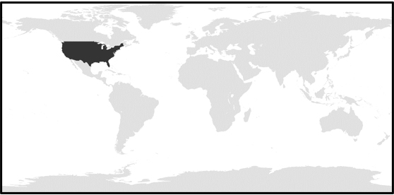
Figure 1.
The contiguous US, highlighted in black.
2.Study area and data
2.1Study area – Contiguous US
The paper uses the contiguous US as the study area (Fig. 1), which includes the continental US excluding the states of Alaska and Hawaii or US territories. The contiguous US was used because the available input data is limited to this area. In terms of US agricultural production, corn and soybeans represent the two largest crops planted by acreage for this study area, which was used to assess the CSB.
2.2Cropland data layer (CDL)
The CDL is a 30-meter pixel-based gridded dataset that represents all landcover across the contiguous US. Currently, the CDL represents over 200 types of crops or cropping patterns with high levels of accuracy for major commodities, such as corn, soybeans, wheat, rice, and cotton. It has been published with complete contiguous US coverage annually since 2008. The two major commodities, corn and soybeans, have accuracies above ninety percent [2]. The CDL has been a useful dataset for agricultural analysis and statistics.
2.3Crop sequence boundaries (CSB)
The coverage of the CSBs consist of the contiguous US. Currently, each of the CSBs are comprised of eight consecutive years of stacked CDLs. The sequence time frame indicates the range of years included in the dataset. Every CSB time frame has unique characteristics based on its input years. For example, the 2015-2022 CSBs include the annual CDL products for the years 2015, 2016, 2017, 2018, 2019, 2020, 2021, and 2022. This paper assessed, a total of eight CSB sequence time frames, across the years spanning 2015 to 2022.
2.4NASS quick stats corn and soybean agricultural estimate data
NASS produces planted acreage estimates for corn and soybeans for most US states; these are considered the ground truth for total planted acres of corn and soybeans at the state and national levels. The planted acreage estimates are available at the end of the season on Quick Stats [29] and are used for validation purposes.
3.Methodology
The approach closely followed the steps described in Beeson et al. 2020, where the first generation of the CSBs (referred to as Crop Management Units) were developed.
By design, the CSB polygons are developed from only publicly available datasets: the NASS CDL [2] and the US Census TIGER line data [30]. The CSB polygons do not use tax parcels, land ownership, or land operator information to define field-level boundaries. The algorithms are an automated python library, arcpy, script utilizing typical GIS tools requiring no manual drawing of CSBs. As fields may divide or combine over years, multiple CSB windows were examined. An eight-year window was used for the first release of the CSBs, but any duration can be used. The initial steps are to filter and simplify CDL classes on each historic CDL year to reduce noise, e.g., misclassified pixels, and re-impose road and rail network line data lost when filtered. These steps are completed in Google Earth Engine (GEE). The resulting rasters are then brought into ArcGIS to be stacked and converted into polygons on a sub-region basis. To address problematic areas, small polygons, under 10,000 m2, are dissolved/eliminated into the neighboring polygon to remove islands within boundaries and clean edges using the ArcGIS eliminate function. The dissolve/eliminate step was developed to preserve areas that are too small to be positively defined as a crop-field. These areas are typically on the edge of a field and are comprised of mixed pixels that can vary year-to-year due to the 30 m pixel resolution of the CDL. This provides further refinement in the CSB to reduce gaps or voids but as a result it increases the area of certain boundaries. Multiple processor environments allow for faster completion of this step as sub-region pools can be spawned to a core when available. Here, the Amazon Web Services (AWS) environment available to the USDA has 96 cores. The resulting CSBs represent areas of similar cropping sequences for the designated years, while separating areas with boundaries that have different cropping sequences. These steps can be repeated for the 8-year moving window to produce the contiguous US resulting in at least eight unique layers of CSB history for all lower 48 states (2008–2015, 2009–2016, 2010–2017, 2011–2018, 2012–2019, 2013–2020, 2014–2021, and 2015–2022).
The CSBs were assessed with original CDL values and USDA NASS official published corn and soybean acreage to calculate percent errors that provide a statistically empirical assessment of the CSB accuracy [29]. The results described will inform readers on the CSBs creation and their accuracies.
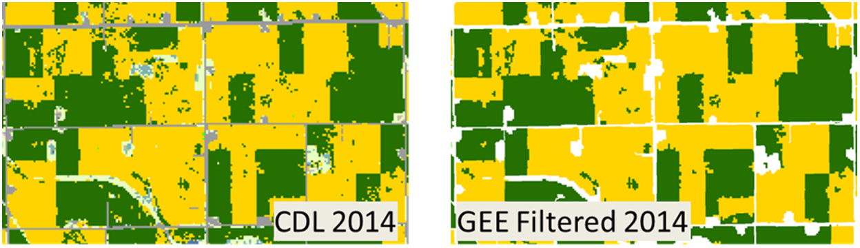
Figure 2.
Comparison of 2014 CDL before (left) and after (right) filtering.
3.1CDL pre-processing
The primary data input to the CSBs is the NASS CDL [2], which is also the input for numerous other field delineation algorithms [5, 6, 7, 8], and [9]. In each of these, the CDL undergoes some degree of pre-processing for two major reasons. First, noise reduction in the CDL is needed. Noise in the CDL is defined as isolated pixels classified with erroneous land cover types because in general CDL accuracies are reported to be between 85% and 95% correct for major crop types [2]. The noise in the CDL is well documented [31] but has been less in the most recent years [32], making noise reduction less important but still useful in earlier years. Second, even in areas with limited noise, simplification is needed given the focus on cropland and the desire to limit the number of unique sequences with stacking multiple years (Fig. 2).
Setting aside some of the important computing steps, four structural changes to the data are made during pre-processing: resampling, reclassifying, filtering, and masking known edge features (roads and railroads).
Resampling: The first change to the raw CDLs is a resampling, which is used to alter pixel size, from 30-meter resolution to 10-meter resolution in Google Earth Engine. The purpose of this step is to improve the masking (reimplementation) of road and rail networks. Because many rural roads and rail routes are less than 30 meters in width, imposing them on a 30-meter gridded dataset introduces errors in field edges, particularly where the transportation features run diagonally across the gridded data. The edge noise, without resampling, leads to a downward bias in boundary calculated areas by assigning too many pixels to roads and rail lines.
Reclassifying: The original CDLs have over 200 different classifications for land covers, so stacking multiple years of CDLs can lead to hundreds of thousands of different unique sequences. The reclassification step aggregates the land cover types into a smaller set of classes. The new classes are based on grouping geographically disparate land cover types together. This keeps the integrity of the crop boundaries in areas with geographical proximity while reducing the quantity of unique sequences. For example, CDL land cover classes for corn and double cropped corn, which include the values corn (1), sweet corn (12), popcorn (13), double cropped winter wheat/corn (225), double cropped oats/corn (226), double cropped triticale/corn (228), double cropped barley/corn (237), and double cropped corn/soybeans (241), are aggregated to one class.
Filtering. A number of other projects have developed alternative methods for filtering and smoothing the CDL [2, 31], and [32]. For the CSBs, the filtering process iterates through multiple steps. First the CDL is filtered using a focal mode based on patch sizes greater than 40 pixels with a radius of four pixels and run with eight iterations. Then the CDL is filtered again (without patch size limits) to reduce speckled CDLs and exaggerate field-shaped boundaries.
Reimposing transportation features: To correct for any misclassification of roads and rails that may have been introduced by the filtering process, or that might have been misclassified in the original CDL, the CSB process uses publicly available transportation feature classes to impose road and rail networks, which are imported from Census Tiger files. The roads are available on GEE, but the rail network has to be uploaded as a local asset.
3.2Zonal identification
Using the modified CDLs for each crop year, the CSBs are developed through six steps: subregion definition, stacking, masking, polygon conversion, refinement, and crop code repopulation.
Subregion definition: Given the large processing requirements for the following steps, each processed CDL is split into subregions. These subregions are defined using the transportation network features. This avoids the problem of splitting CSBs along administrative boundaries (e.g., states and/or counties lines) or biophysical boundaries (e.g., watersheds). The size of the subregion and the number of subregions allows for efficient multi-core processing.
Figure 3.
Creation of sequence zones by stacking eight filtered CDLs (left) and using combine raster function (center), then edge artifact cleaning to final CSBs (right).
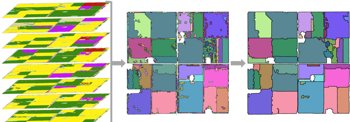
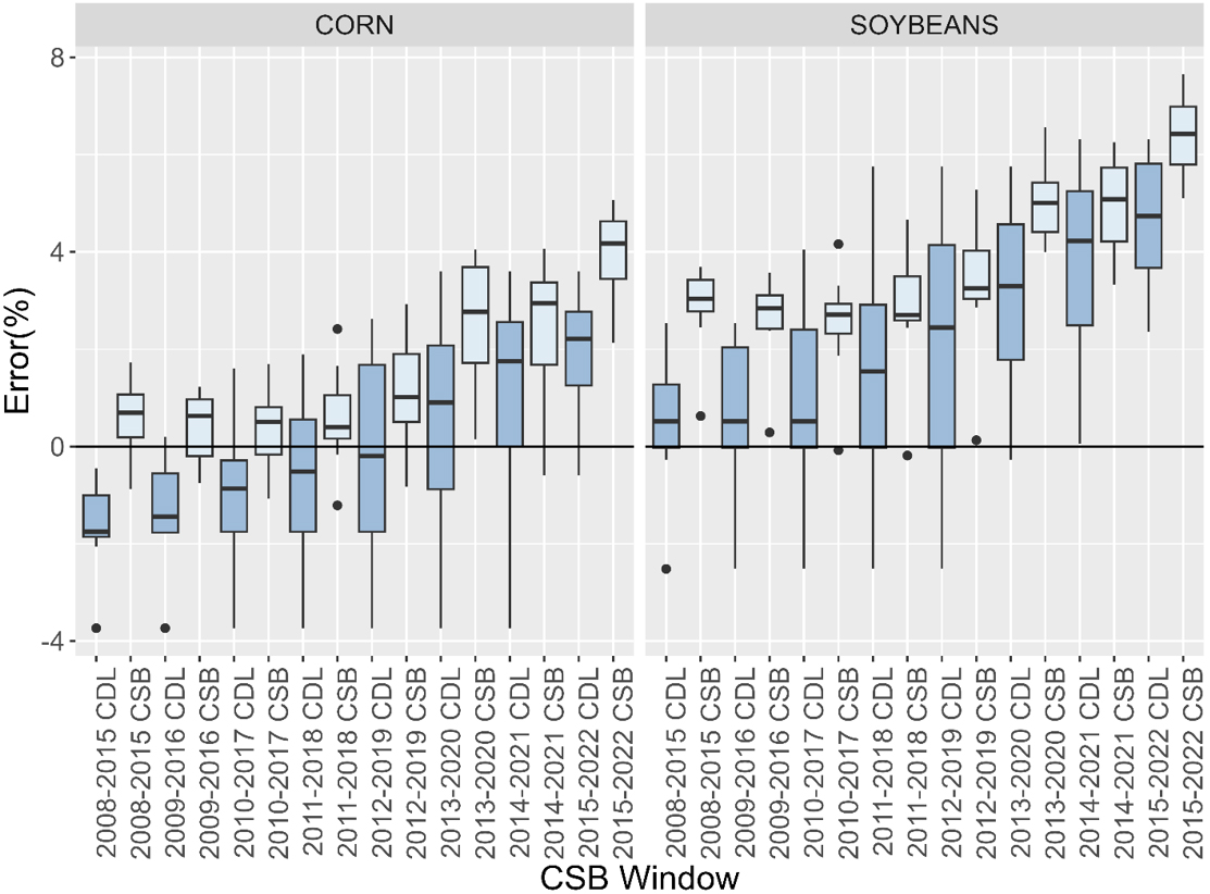
Figure 4.
Box and whisker plot of the CDL and CSB windows and their error to the USDA NASS Quick Stats official planted acreage value for corn and soybean. Each box is made up of the eight years used in the associated CSB window.
Stacking:The current CSBs are developed using a stack of eight CDL years, but any duration could be used (Fig. 3). A shorter window, using fewer years, will result in larger polygons that may not divide similar cropping areas as much. A longer window, using more years, will result in smaller polygons that possibly divide the area more than expected. If a project spans a 10-year period, it would be appropriate to use the same 10-year window CSB to match. If a project studies rotations on a 3-year basis, then a CSB window in multiples of three would be appropriate (e.g., 3, 6 or 9 years). The 8-year window was chosen as a good compromise for not over or under dividing with the results most resembling fields.
Masking: All sequences that do not involve any crop classes or only one year of cropping are removed. These areas may be forest, pasture, or developed land cover types, to name a few.
Polygon Conversion: Each zone of adjacent pixels with the same sequences are converted into polygons. In addition to aggregating (joining) similar pixels, the conversion step simplifies the polygons to reduce the number of extra vertices. The polygons are projected to Albers Conical to prevent adding artifacts that look like steps in otherwise straight lines while in raster format. The original raster files exported from Google Earth Engine are in Geographic projection (WGS1984), which reduces the stairstep appearance of the roads and rails because in the US most of them were constructed on longitude and latitude lines. Once polygons they can be projected without introducing these unwanted artifacts.
Refinement: The ArcGIS Pro eliminate function was used to avoid downward bias in area, thus preserving the aggregate total area as much as possible, resulting in a continuous border between CSB polygons. The model runs elimination four times to dissolve problematic areas into larger neighboring polygons. The first time the selected polygons are less than 100m2; in the second they were less than 1,000m2; and for the last two, the polygons are less than 10,000m2.
Repopulating: Repopulating the attribute table uses zonal majority of CDL classes as well as county and state locations. A unique ID is added after all sub-regions are joined.
3.3CSB acreage validation
One way of validating the accuracy of the CSBs is to compare the CSB derived acreage to the available ground truth planted acreage and against the original CDL. Ground truth data are available for a wide range of crops on the USDA NASS Quick Stats website. Planted acreages on Quick Stats are available at the county, state, and national levels.
To calculate the CSB-based acreage, a crop type is assigned to each CSB based on the majority class of CDL pixels within each polygon. For a given state and crop, the CSB-derived, state-level planted acreage is the sum of the areas of each CSB within the state containing the crop of interest (1)
(1)
where,
Once the state and national estimates are obtained from the CSBs, the error can be calculated using the percent error:
where PE is the percent error and
4.Results and discussion
This paper described the CSB creation methodology by defining the steps to the algorithm and their importance to its development. The computationally intense process described successfully combines multiple publicly available geospatial datasets into a single geospatial output file for the contiguous US. The resulting file was assessed with original CDL values and officially published corn and soybean acreage to calculate percent errors that provide an empirical assessment of the CSBs accuracies. The results described in this section will inform readers on the CSBs creation and their accuracies.
Initial 8-year CSB creation for the contiguous US took about five days using a 96-core AWS workstation. The process is fully automated, but the sizes of the 86 subregions are not balanced. Some sub-processing regions are completed in a couple hours while a few takes five days. This could be improved to reduce the time to two days. A majority of the processing time was spent on the dissolve/elimination step (ArcGIS Pro eliminate function), which incrementally
Table 1
Percent error for CSB’s compared to Quick Stats national planted acreage for corn and soybean
| Corn | Soybean | |||||
|---|---|---|---|---|---|---|
| Year | Quick stats (ac) | CSB (ac) | Error | Quick stats (ac) | CSB (ac) | Error |
| 2015 | 88,019,000 | 89,888,422 | 2.1% | 82,660,000 | 87,120,721 | 5.4% |
| 2016 | 94,004,000 | 96,665,222 | 2.8% | 83,453,000 | 87,644,495 | 5.0% |
| 2017 | 90,167,000 | 93,440,276 | 3.6% | 90,162,000 | 96,119,359 | 6.6% |
| 2018 | 88,871,000 | 92,904,634 | 4.5% | 89,167,000 | 95,515,323 | 7.1% |
| 2019 | 89,745,000 | 93,459,732 | 4.1% | 76,100,000 | 80,548,849 | 5.8% |
| 2020 | 90,652,000 | 95,060,605 | 4.9% | 83,354,000 | 88,401,544 | 6.1% |
| 2021 | 93,252,000 | 97,139,581 | 4.2% | 87,195,000 | 93,138,351 | 6.8% |
| 2022 | 88,579,000 | 93,071,290 | 5.1% | 87,450,000 | 94,088,968 | 7.6% |
reduces the number of total polygons (Fig. 3). This step is run four times by dissolving the selected polygons into the neighbor that shared the longest border. The first dissolve/elimination process started at nearly 500 million polygons and dissolved about 100,000 that were less than 100 m2. The second pass selected 250 million polygons that were less than 1,000m2. The third pass selected another 100 million polygons that were less than one hectare. The last pass started with over 50 million polygons and reduced the remaining by 50 percent. After the dissolve/elimination step, only polygons greater than one hectare were kept as final CSBs which reduced the resulting 25 million polygons to fewer than 20 million. Absent incrementally increasing the selection size, the tool often fails or takes days. Without this step the polygons only cover about 100,000,000 hectares which is about 34,000,000 hectares shy of the reported US cropland area. With this step, the CSBs report about 8,000,000 hectares over the expected US acreage for 2022.
Figure 5.
CSB corn planted acreage compared to Quick Stats by state (fit line is dashed and the one-to-one line is solid).
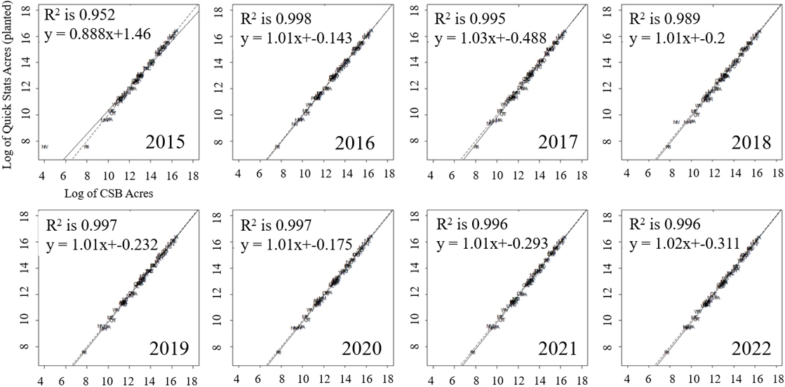
The area totals for each crop follow the accuracy of the initial CDL input. In general, compared to the USDA NASS Quick Stats national acreage, values produced by the CSB are higher than the CDL (Fig. 4). This is due to the elimination step forcing the polygons to match their neighbors’ edges by expanding into mixed pixels of non-cropland or edge noise. Nationally the CSB values for corn and soybean acreage are consistently greater the official estimates from Quick Stats (Table 1). For corn, the percent error increases with time. The percent error for soybeans tends to increase with time, though it varies. Prior to 2019 the CDLs typically underpredict crop acreages the elimination step helps the CSBs replicate the Quick Stats values to a closer degree (Table 1). In later years, after 2019, the CDL improved methods for classifying mixed pixels, giving weight for those pixels to be classified as cropland ultimately overestimating Quick Stats values. This trend of overestimating is preserved as it is a derivative product of the CDL.
When CSB acreage for corn at the state level was compared to Quick Stats reported planted corn acres, the results are generally the same nationally by tending to overestimate like the CDL (Fig. 5). The CSB acreage was higher with a slope value above 1.0 with few outliers at the lower values. However, the earliest year, 2015, had a lower slope value at 0.888. The largest outlier was Nevada and has under reported values in 2015 and 2018.
Figure 6.
CSB soybean acreage compared to Quick Stats by state (fit line is dashed and the one-to-one line is solid).
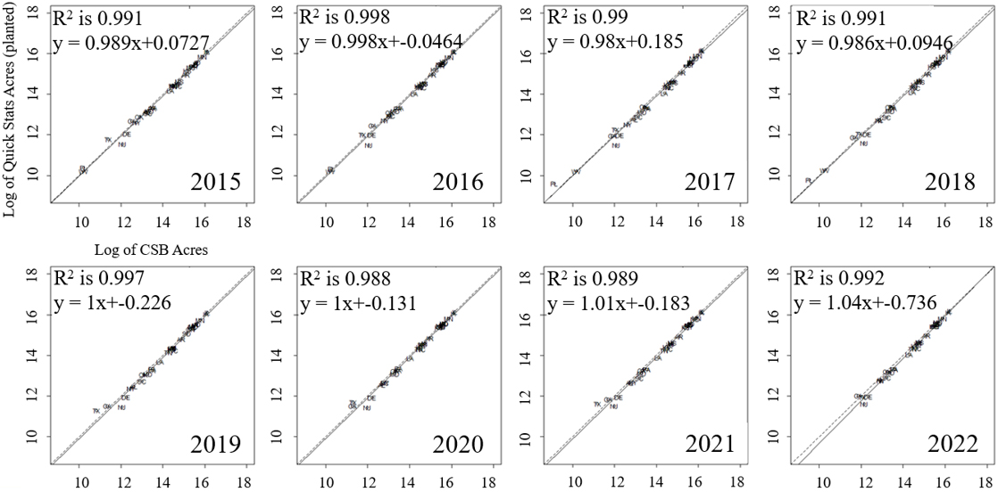
For soybean CSB acreage at the state level, the slope value has trended above 1.0 in the last several years (Fig. 6). Generally, soybeans have greater outliers in both higher and lower acreage than Quick Stats but continue to follow the national trend and generally overestimate. Some of the outlier states with lower CSB areas are Texas, Oklahoma, and Florida. New Jersey and Delaware are outliers in the positive direction. Soybeans tend to have a wider range of results, and the r2 value is slightly lower than that for corn.
4.1CSB uses
In Abernethy et al. 2023 [33], a field-level model for pre-season crop type prediction using CSBs was introduced. The CSBs served as field analogs in a machine learning model leveraging historical crop rotations to predict the crop to be planted for the current year. CSB-based predictions were shown to be competitive with previous pixel-based forecasting models when compared to FSA CLU ground-reference data, and at a reduced computational burden. Crop type summaries by CSBs provide a computational efficient procedure for crop type forecasting over a large area [33].
Another study has started to use the CSBs to validate the imputation work from NRCS Conservation Effects Assessment Project (CEAP) Agricultural Policy Environment eXtender model (APEX) data. They verified the rotation/crops that were imputed from the CEAP survey data to additional NRI points/locations using the CSB. There was a strong correlation (96%) between the data provided by the surveyed farmers and the sequence of crops derived by CBSs, reinforcing the reliability and accuracy of the data collected.
USDA NASS used the CSBs to identify potential new farms to include in the National Agricultural Classification Survey (NACS). The number of potential farms identified through this process varied with state, exceeding 28,000 in Florida [34]. The NACS is used to determine the farm status of the potential farms. Most of them do not meet the definition of a farm, which is any operation that produces or has the potential to produce at least $1000 in a year. However, each farm identified improves the coverage of the NASS list frame.
USDA ARS used the CSBs to create crop rotation summaries for management file input to a carbon model using Markov Chain. There are millions of possible crop sequences across the US. By summarizing them into several dozen options, the model input files are manageable while minimally affecting model response. This method would be useful to other modeling efforts, and rotation summaries could be included in future CBS attribute tables. CSBs are used the same way in the Nitrogen Recommendation Tool for precision nutrient management in OK and KS [35].
Furthermore, CSBs are being considered to support mapping of winter cover crop presence/absence in the contiguous US the USDA greenhouse gas assessment. USDA ARS and USGS are comparing CSBs with additional field boundary polygons, public and private, to assess accuracy and applicability for remote sensing of agricultural land cover (cover crops, tillage intensity).
4.2CSB limitations
CSBs are a derivative product of the CDL and will propagate misclassifications found in the CDL. While this was reduced by filtering and reclassifying the CDL during CSB creation, false islands and bands in otherwise continuous fields will exist. Users can identify and dissolve those features if they wish to reduce unwanted features, but this might change the area totals reported. Additionally, there are artifacts from converting raster formatted products to polygon features that retain grid shapes when a straight line is warranted. This presents as CSB not describing the field perfectly which is acceptable because these are polygons of continuous cropping sequences as seen in the CDL, not field boundaries. Users can smooth the CBSs to match their needs, but again may introduce new errors to the area totals. Future versions of the CSB will minimally smooth the polygons, but a certain amount of grid shapes will remain to not introduce large errors. Overall, CSBs can enhance the signal and reduce the noise of remotely sensed data to supply the full population versus a sample for a more complete description.
5.Conclusions
Creation of the CSBs is a repeatable automated process for building crop-field polygons with accurate representation of crop areas. Geospatial research into automatic crop-field delineation has been studied for many years; however, with advancements in accessibility to cloud computing and a growing historical CDL archive, it is now possible to produce the contiguous US products demonstrated in this paper using this method.
The CBSs were designed to be flexible and customizable. Users can extract their specific study areas from the contiguous US files, further refine the polygons to reduce certain CDL artifacts, and spatially join other datasets to the CBS attribute table to perform previously difficult spatial analyses. In addition, if the settings used to create the publicly available CSBs (https://www. nass.usda.gov/Research_and_Science/Crop-Sequence-Boundaries) differ from users’ needs, they can create their own using the code provided on the GitHub site (https://github.com/USDA-REE-NASS/csb-project).
The CSBs may benefit from future refinement. The current version represents an early iteration, prioritizing a uniform spatial and temporal methodology. This produces a streamlined product but likely at the cost of accuracy for some geographical areas due to unique factors that vary across physical landscapes. The current methods were focused on representing field-level boundaries and crop sequences with fixed computing resources to complete this study. The CSBs may be improved by using other inputs beyond the CDL like additional satellite imagery or administrative data. They can be improved by expanding the methods to more complex algorithms and tuning for local variability at the state level. Additionally, improvements in the CDL like going to 10-meter resolution may improve field-level polygons. These new considerations and advancements could enhance CSB accuracy.
This approach can provide a solid methodology for advancing automatic crop-field delineation in the US and around the world. The CSBs have been useful with some recent examples including predicting preseason planted acreage, verifying crop types and rotations, identifying potential farms for new survey participants, and determining survey reliability. We believe this will be useful for other types of studies and can be utilized by researchers with needs for field-level polygons depicting agricultural land cover in the U.S.
Disclaimer
This research was supported by the U.S. Department of Agriculture, Economic Research Service and National Agricultural Statistics Service. The findings and conclusions in this publication are those of the author(s) and should not be construed to represent any official USDA or U.S. Government determination or policy.
References
[1] | National Academies of Sciences, Engineering, and Medicine. Principles and Practices for a Federal Statistical Agency: Sixth Edition. Washington, DC: The National Academies Press. (2017) ; doi: 10.17226/24810. |
[2] | Boryan C, Yang Z, Mueller R, Craig M. Monitoring US agriculture: the US Department of Agriculture, National Agricultural Statistics Service, Cropland Data Layer Program. Geocarto International. (2011) ; 26: (5): 341-58. |
[3] | Boryan CG, Yang Z, Willis P. US Geospatial Crop Frequency Data Layers, Proc. of the Third International Conference on Agro-geoinformatics. August 11–14, (2014) , Beijing, China, doi: 10.1109/Agro-Geoinformatics.2014.6910657. |
[4] | Boryan, CG, Yang, Z, Di L. Deriving 2011 Cultivated Land Cover Data Sets Using USDA National Agricultural Statistics Service Historic Cropland Data Layers. Proc. of IEEE International Geoscience and Remote Sensing Symposium, July 22–27, (2012) , Munich, Germany. |
[5] | Yan, L and Roy DP. Automated crop field extraction from multi-temporal Web Enabled Landsat Data. Remote Sensing of Environment. (2014) ; 144: : 42-64. |
[6] | Beeson, PC, Daughtry, CS, Wallander, SA. Estimates of conservation tillage practices using landsat archive. Remote Sensing. (2020) ; 12: (16): 2665. |
[7] | Rahman MS, Di L, Yu Z, Eugene GY, Tang J, Lin L, Zhang C, Gaigalas J. Crop Field Boundary Delineation using Historical Crop Rotation Pattern. In 2019 8th International Conference on Agro-Geoinformatics. IEEE Agro-Geoinformatics. 2019: : 1-5. |
[8] | Jong M, Guan K, Wang S, Huang Y, Peng B. Improving field boundary delineation in ResUNets via adversarial deep learning. International Journal of Applied Earth Observation and Geoinformation. (2022) ; 112: : 102877. |
[9] | Yan L, Roy DP. Conterminous United States crop field size quantification from multi-temporal Landsat data. Remote Sensing of Environment. (2016) ; 172: : 67-86. |
[10] | Ji CY. Delineating agricultural field boundaries from TM imagery using dyadic wavelet transforms. ISPRS Journal of Photogrammetry and Remote Sensing. (1996) ; 51: (6): 268-83. |
[11] | Cheng T, Ji X, Yang G, Zheng H, Ma J, Yao X, Zhu Y, Cao W. DESTIN: A new method for delineating the boundaries of crop fields by fusing spatial and temporal information from WorldView and Planet satellite imagery. Computers and Electronics in Agriculture. (2020) ; 178: : 105787. |
[12] | Xu L, Ming D, Du T, Chen Y, Dong D, Zhou C. Delineation of cultivated land parcels based on deep convolutional networks and geographical thematic scene division of remotely sensed images. Computers and Electronics in Agriculture. (2022) ; 192: : 106611. |
[13] | Graesser J, Ramankutty N. Detection of cropland field parcels from Landsat imagery. Remote Sensing of Environment. (2017) ; 201: : 165-80. |
[14] | Garcia-Pedrero A, Gonzalo-Martin C, Lillo-Saavedra M. A machine learning approach for agricultural parcel delineation through agglomerative segmentation. International Journal of Remote Sensing. (2017) ; 38: (7): 1809-19. |
[15] | Masoud KM, Persello C, Tolpekin VA. Delineation of agricultural field boundaries from Sentinel-2 images using a novel super-resolution contour detector based on fully convolutional networks. Remote Sensing. (2019) ; 12: (1): 59. |
[16] | Wagner MP, Oppelt N. Extracting agricultural fields from remote sensing imagery using graph-based growing contours. Remote Sensing. (2020) ; 12: (7): 1205. |
[17] | Wagner MP, Oppelt N. Deep learning and adaptive graph-based growing contours for agricultural field extraction. Remote Sensing. (2020) ; 12: (12): 1990. |
[18] | Taravat A, Wagner MP, Bonifacio R, Petit D. Advanced fully convolutional networks for agricultural field boundary detection. Remote Sensing. (2021) ; 13: (4): 722. |
[19] | Persello C, Wegner JD, Hänsch R, Tuia D, Ghamisi P, Koeva M, Camps-Valls G. Deep learning and earth observation to support the sustainable development goals: Current approaches, open challenges, and future opportunities. IEEE Geoscience and Remote Sensing Magazine. (2022) ; 10: (2): 172-200. |
[20] | Waldner F, Diakogiannis FI, Batchelor K, Ciccotosto-Camp M, Cooper-Williams E, Herrmann C, Mata G, Toovey A. Detect, consolidate, delineate: Scalable mapping of field boundaries using satellite images. Remote Sensing. (2021) ; 13: (11): 2197. |
[21] | Estes, LD, Ye S, Song L, Luo B, Eastman JR, Meng Z, Zhang Q, McRitchie D, Debats SR, Muhando J, Amukoa AH. High resolution, annual maps of field boundaries for smallholder-dominated croplands at national scales. Frontiers in Artificial Intelligence. (2022) ; 4: : 744863. |
[22] | Hong R, Park J, Jang S, Shin H, Kim H, Song I. Development of a parcel-level land boundary extraction algorithm for aerial imagery of regularly arranged agricultural areas Remote. Sensing. (2021) ; 13: (6): 1167. |
[23] | Kumar S, Jayagopal P. Delineation of field boundary from multispectral satellite images through U-Net segmentation and template matching. Ecological Informatics. (2021) ; 64: : 101370. |
[24] | Turker M, Kok EH. Field-based sub-boundary extraction from remote sensing imagery using perceptual grouping. ISPRS Journal of Photogrammetry and Remote Sensing. (2013) ; 79: : 106-21. |
[25] | Li T, Johansen K, McCabe MF. A machine learning approach for identifying and delineating agricultural fields and their multi-temporal dynamics using three decades of Landsat data. ISPRS Journal of Photogrammetry and Remote Sensing. (2022) ; 186: : 83-101. |
[26] | Waldner F, Diakogiannis FI, Batchelor K, Ciccotosto-Camp M, Cooper-Williams E, Herrmann C, Mata G, Toovey A. Detect, consolidate, delineate: Scalable mapping of field boundaries using satellite images Remote. Sensing. (2021) ; 13: (11): 2197. |
[27] | Fritz S, See L, McCallum I, You L, Bun A, Moltchanova E, Duerauer M, Albrecht F, Schill C, Perger C, Havlik P. Mapping global cropland and field size. Global Change Biology. (2015) ; 21: (5): 1980-92. |
[28] | USDA Farm Service Agency. Common Land Unit (CLU) Information Sheet April 12, (2012) . Available from: https//www.fsa.usda.gov/Internet/FSA_File/clu__infosheet_2012.pdf. [Accessed 28 March 2024]. |
[29] | USDA National Agricultural Statistics Service. NASS – Quick Stats. USDA National Agricultural Statistics Service. Available from: https://data.nal.usda.gov/dataset/nass-quick-stats [Accessed: 29 March 2023]. |
[30] | 2019 TIGER/Line Shapefiles (machine readable data files)/prepared by the US. Census Bureau, (2019) . |
[31] | Lin L, Di L, Zhang C, Guo L, Di Y, Li H, Yang A. Validation and refinement of cropland data layer using a spatial-temporal decision tree algorithm. Sci Data. (2022) ; 9: (1): 63. doi: 10.1038/s41597-022-01169-w. |
[32] | Lark T, Mueller R, Johnson D, Gibbs H. Measuring land-use and land-cover change using the US. department of agriculture’s cropland data layer: Cautions and recommendations. International Journal of Applied Earth Observation and Geoinformation. (2017) ; 62: : 224-35. doi: 10.1016/j.jag.2017.06.007. |
[33] | Abernethy J, Beeson PC, Boryan CG, Hunt KA, Satore L. Preseason crop type prediction using crop sequence boundaries. Computers and Electronics in Agriculture. (2023) ; 208: : 107768. ISSN 0168-1699, doi: 10.1016/j.compag.2023.107768. |
[34] | Jennings R. Georeferencing Process [WWW Document]. Esri Map Gall. Available from: https//www.esri.com/en-us/about/events/uc/agenda/virtual-map-gallery#/submission-detail/62cb72d2ff6b1a12e0ccfbf0. [Accessed 29 March 2023]. |
[35] | Chen X, Chambers RG, Bandaru V, Jones C, Ochsner T, Witt T. Precision Nitrogen Management for Winter Wheat Under Price and Weather Uncertainty. (in review) Available at SSRN: https://ssrn.com/abstract=4435286; or doi: 10.2139/ssrn.4435286. |


