Multivariate small area estimation of undernutrition for children under five using official statistics

1.Introduction

Sample surveys are mainly designed to produce estimates of population characteristics of interest for larger domains at regional and national levels with large sample sizes [1]. In these large domains, reliable, efficient, and precise direct survey estimates can be produced from the survey data. However, in many practical cases, estimates are often required for areas with small sample sizes for which the survey was not addressed. Recently the demand for reliable, consistent, and precise small area statistics is significantly increased across the globe. Unfortunately, for most surveys, the sample size is not large enough to guarantee reliable direct estimates for all characteristics of interest. Small area estimation (SAE) overwhelmed the problems of producing reliable estimates of parameters of interest for which the samples sizes are too small for adequate precisions [1].

Small area estimations based on area-level aggregated population data is a Fay Herriot model since it was introduced by [2]. Many researchers studied small area estimation under the univariate Fay Herriot (UFH) model, which overlooks the correlation between related target variables of interest [3, 4, 5]. However, surveys may be appropriate in practical cases to consider many correlated target variables. In such cases, the multivariate Fay-Herriot (MFH) model can be used to integrate the correlation among target variables. The MFH extends the UFH model introduced by [6] and developed by considering different covariance structures of the random effects by [7]. The MFH model replicated the joint modeling of more than one target variable, in contrast to the UFH model [8]. MFH models have become popular methods to produce reliable parameter estimates of multiple related characteristics of interest that are commonly produced from many surveys [8].

Statisticians are often applied to assess correlated measures of target variables, such as undernutrition indicators (stunting, wasting, and underweight). Multivariate models consider the correlation of different variables and are typically applied to this situation. There are few publications in the literature on small area estimates that use multivariate small area estimations under the FH model. Studies by [7, 8, 9, 10] evaluated the precision of small area estimators produced from univariate models to those generated from multivariate models for each target variable.

In this study, we used a multivariate extension of the Fay-Herriot model to help the estimate of mean vectors of the z scores of undernutrition indicators in small areas for small or zero sample sizes. When multiple dependent variables are considered correlated, the MFH model may produce better results than the univariate FH model [1], but these models have received little attention.

The mean squared error (MSE) is integral to small area estimation research [1]. MSE estimation depends on the method of model parameter estimation, but the assumptions made about the distributions of the random model components. It is essential to obtain an accurate estimator of MSE to reflect the true variability associated with the EBLUP estimators. MSE estimators have been studied using variance component estimators under the MFH model [11, 12]. The performance of small area estimates under the MFH model was assessed by the coefficient of variation (CV %) and root MSE [10, 13].

Undernutrition remains the leading public health problem in different continents, especially in eastern Africa and southern Asia [14, 15]. In Ethiopia, undernutrition is a severe problem for children under five and table among the worst countries in the world [16, 17]. Even though there has been significant recent progress in the country, there are still problems in different parts [16]. The target variable for this study has been the z-score of the undernutrition status of children under five, which are underweight (weight-for-age), stunting (height for age), and wasting (weight for height) from the 2016 Ethiopian demographic and health survey (EDHS) data.

The standardized measures of stunting, wasting, and underweight were calculated using the new child growth standards released by the world health organization [18]. Children whose height-for-age z-score is below minus two standard deviations (-2 SD) from the median of the reference population are considered stunted, which means low height relative to age. Children whose weight for height z-score is below minus two standard deviations (-2 SD) are deemed to be wasted [15, 17, 18]. Underweight is a composite form of undernutrition that includes elements of stunting and wasting. If the weight for age z-score is below minus two standard deviations (-2 SD), then the child is underweight [17, 18].

According to the report in [15], globally, an estimated 144 million and 47 million children under five were stunted and wasted, respectively. Most of the world’s stunted, underweight and wasted children under five were lived in Asia and Africa [15]. In Ethiopia, 38%, 10%, and 24% of children under five were stunted, wasted, and underweight [16, 17].

Many studies in Ethiopia examined undernutrition at the regional level [16, 19, 20, 21, 22, 23, 24]. These analyses were carried out utilizing survey data from planned domains at the national and regional levels. Furthermore, some studies have recently been undertaken at the zonal level [25, 26, 27]. However, the small area estimation ideas that boost effective sample sizes were overlooked in these investigations. As a result, unplanned areas that are zones of undernutrition in Ethiopia (the third administrative level) must be assessed using auxiliary variables to overcome the problem of small sample sizes. Because of the small sample size and the fact that the zones are unplanned domains for the Ethiopian survey, traditional direct survey estimation methods cannot be employed. As a result, under the MFH model, small area estimations are applied for under five age child undernutrition indicators.

The health service uses decentralization as the most influential administrative determinant [28]. The federal ministry of health decentralized the health service parallel to the government structures (regions, zones, and woredas). These administrative hierarchies are the key institutions involved in health care delivery in the country [28, 29]. Among them, the zonal governments serve as a bridge between regional and woreda (district) governments. The zonal health department is responsible for monitoring and evaluating health activities in the districts [28], which means that zones have more policy implications than districts. Therefore, zonal level estimates of undernutrition are invaluable for legislative organs at any level of structures in the country.

Thus, our study was focused on the multivariate estimates of the z scores of undernutrition (stunting, wasting, and underweight) of the zones to produce relatively the best reliable, efficient, and precise estimates, viz. borrowing auxiliary variables from the census data under the MFH model. A z-score, also known as standard deviation from the mean, is a measure of data dispersion, with some data being highly dispersed and others being less so. Z scores allow researchers to compare data from several normally distributed samples. It also provides several advantages. The most noteworthy is that they may be used to estimate summary statistics for the population or subpopulations, such as CV and quartiles [18, 30, 31].

The successive sections of this research paper are organized as follows: Section 2 describes the data sources, the sampling design and methodologies of the multivariate Fay Herriot model, Section 3 contains the results, discussions are presented in Section 4, and finally, Section 5 contains conclusions.

2.Methods and materials

In this section, the secondary source of the data used in the MFH model was the 2016 EDHS combined with the 2007 population and housing census data. These were the latest round of available data being used for policymakers in Ethiopia. A wide gap could exist between the 2007 census and 2016 survey data since the census in this country takes place every ten years. Note that using auxiliary covariates to model the undernutrition data from 2016 data are not expected to change significantly over a short period of time [32]. However, we used the 2016 census projection for sex, urban and rural residence auxiliary variables to all zones [33].

These data are used for estimating the z-scores of undernutrition at zonal levels in Ethiopia. The 2016 EDHS used a sampling frame designed for the Ethiopian population and housing census, which was carried out in 2007 by the Ethiopian central statistical agency (CSA). The 2016 sample survey was designed to provide reliable estimates of key indicators at the national and regional levels. Similarly, the sample survey was designed to provide estimates for urban and rural areas [17].

In the 2016 EDHS, a two-stage stratified random sampling technique was applied to collect data from nine regions, two administrative cities, and urban and rural areas. There were 21 strata selected for sampling. Enumeration areas (EAs) samples were collected independently from each stratum in two stages. At every lower level of administration, implicit stratification and proportional allocation were achieved by sorting the sampling frame within each sampling stratum before sampling, according to administrative units at different levels, and using a probability proportional to sample size selection at the first sampling stage [17].

In the first stage, 645 EAs were independently selected in each stratum with probability proportional to the EAs size. Among 645 EAs, 202 EAs were for urban, and 443 EAs were for rural areas. In the second stage, an equal probability systematic sampling was used to select 28 households per cluster from the newly created household lists. The height and weight measurements were collected from children 0–59 months, women aged 15–49 years, and men aged 15–59 years [17] in all the selected households. In this study, we comprised 8441 households of children under five within 87 zones of Ethiopia. The sample sizes are ranged from 5 to 457 households, with an average of 97 households in all 87 surveyed areas (zones special zones and special woredas). And also, there were eight non-sampled zones (special zones and special woredas).

2.2Multivariate Fay Herriot model

Various extensions of the basic area-level model have been developed in the literature [1, 7, 8, 11, 12]. One type of extension leads to extending the UFH model to a multivariate Fay-Herriot model to take advantage of the correlations between different characteristics of interest [7, 8]. Suppose the population is decomposed into m areas. Let 𝜽j= (θ1⁢j, θ2⁢j, …, θm⁢j)T be a vector of the jt⁢h characteristics of interest and 𝒚j=(y1⁢j,y2⁢j,…,ym⁢j) be the jt⁢h estimators of 𝜽j, with j= 1, 2, …⁢J. The MFH is defined in two stages. The first stage is the sampling model which is given below

(1)

𝒚j=𝜽j+ϵj,j=1,2,…,J=3

Where the vector ϵj∼N⁢(0,𝑹j) is a sampling error with known m×m covariance matrix Vj. Moreover, we can assume that νj is related to pj area-specific auxiliary variables 𝒙j=𝒙1,…,𝒙J)T. Through a linking model.

(2)

𝜽j=𝒙jT⁢𝜷j+𝝂j,𝝂j∼N⁢(0,Gj),j=1,J

where 𝝂j=(𝝂1⁢j,𝝂2⁢j,…,𝝂m⁢j)T be a vector of area (zone) random effects with J×J covariance matrix Gj=σj2⁢𝑰m where 𝑰m is m×m identity matrix for i=1,2,…,m. The matrix 𝒙j be the jt⁢h matrix of area level auxiliary variables of size m×pj and 𝜷j=(𝜷1,𝜷2,…,𝜷J) be vector of regression coefficients corresponding to 𝒙j. Therefore, combining the sampling and linking models, the multivariate Fay Herriot model is produced as follows.

(3)

𝒚j=𝒙j⁢𝜷j+𝝂j+ϵj,j=1,2,…,J=3

where 𝝂j∼N⁢(0,Gj) and ϵj∼N⁢(0,𝑹j) with 𝝂j and ϵj are independent, and 𝒚j is the direct estimates of the target variables of interest. Where J is the number of target variables.

We can rewrite model (3) in matrix form as follows

(4)

𝒚=𝒙⁢𝜷+𝒛⁢𝝂+ϵ,𝝂∼N⁢(0,𝑮),ϵ∼N⁢(0,𝑹)

where 𝝂=𝑐𝑜𝑙1⩽j⩽J⁢(𝝂j) and ϵ=𝑐𝑜𝑙1⩽j⩽J⁢(ϵj) are independent. The matrix z is a constant matrix assumed to be known. The matrix 𝒙=𝑑𝑖𝑎𝑔1⩽j⩽J⁢(𝒙j) is 𝐽𝑚×pj matrix of area level auxiliary variables (area level proportions), 𝒚=𝑐𝑜𝑙1⩽j⩽J⁢(𝒚j) is J⁢m×1 vector of variable of characteristics interest (target variables). The col operator means stacking the matrix column. Gs is the covariance matrix of area effects, and also Rs is the sampling errors of the JmxJm covariance matrix, which is assumed to be known from the survey data.

In our study the characteristics interest of target variables were stunting (yi⁢1), wasting (yi⁢2) and underweight (yi⁢3) obtained from 2016 EDHS survey data. The direct survey estimator of a total yi⁢j=∑n=1Niy𝑖𝑗𝑛 is y^i⁢j𝑑𝑖𝑟=∑wi⁢n⁢y𝑖𝑗𝑛. Where n is the sample and wi⁢ns are the sampling weights of the nt⁢h household within the it⁢h area, j=1,2,…⁢J=3, n=1,2,…,Ni, i=1,2,…,m. The direct estimator of the it⁢h area population is N^i𝑑𝑖𝑟=∑wi⁢n. The direct weighted survey estimator of the area mean is y¯i⁢j=y^i⁢j𝑑𝑖𝑟/N^i𝑑𝑖𝑟 [2, 3].

Therefore, the direct estimator of the variance covariance matrix (R) of the multivariate data for z scores of stunting (yi⁢1), wasting (yi⁢2) and underweight (yi⁢3) were approximately in the following equations.

𝐶𝑜𝑣⁢(y¯i⁢l,y¯i⁢r)=(1Ni)2⁢∑

wi⁢n⁢(wi⁢n-1)⁢(y𝑖𝑙𝑛-y¯i⁢l)⁢(y𝑖𝑟𝑛-y¯i⁢r)

where l,r=1,2,3, n=1,…,Ni, i=1,…,m. wi⁢n are the sampling weights of the nt⁢h household within the it⁢h area [4].

This study considered three particularizations of models under the Fay Herriot model in Eq. (4) concerning the arguments of correlated characteristics of interest. The first model is assumed to have zero correlation between the target variables (stunting, wasting, and underweight). This is particularly the UFH model. The second model is a model that assumed the existence of correlations with the homogeneity of the covariance matrix of the area-level random effects. Therefore, in model two, the model variance component parameters are the correlation (ρ) and the homogeneous variance (𝑮=σν2).

The area level (zonal level in our case) random component ν∼N(0,G=σν2) in model (4) is for each area level random component, νi∼N⁢(0,σν⁢i2), since all area level components are not homogeneous [2, 4, 5]. The second model, the autoregressive multivariate Fay-Herriot model (AR (1)), has been written as follows:

σν⁢i2=σν2⁢Ωi⁢(ρ),i=1,2,⋯⁢m

Ωi⁢(ρ)=11-ρ2⁢[1ρ⋯ρR-2ρR-1ρ1⋯ρR-3ρR-2⋮⋮⋱⋮⋮ρR-1ρR-2⋯ρ1]

Correlations (ρ) are highest between neighboring times in the first order autoregressive (Lag 1) structure, and decrease systematically with increasing distance between time points.

The last model is the heteroscedastic version of the second model, such that there exist correlations with heterogeneous random variances components. Model 3 is known as the heteroscedastic autoregressive multivariate Fay-Herriot model (HAR(1)), and its random error component is as follows [7, 8]:

ν(i⁢r)=ρ⁢νi⁢r-1+αi⁢r,νi⁢0∼N⁢(0,σ02),αi⁢r∼N⁢(0,σr2),r=1,2,…,R,i=1,2,…,mσν⁢02=1,αi⁢r, and νi⁢0 are independent and the elements of random variance matrix is written as σ𝑖𝑟𝑗𝑗=∑k=1j=ρ2⁢k⁢σj-k2, for diagonal matrix σ𝑖𝑟𝑗𝑠=∑k=0j-sρ2⁢k+|j-s|⁢σ|j-s|-k2, for the off diagonal matrix

2.2.1Multivariate small area estimates under Fay Herriot model

The MFH in model (4) can be written in the form of general linear mixed model [6]. The multivariate empirical best linear unbiased prediction (EBLUP) of area level random effects are (ν=col1⩽i⩽m(νi)) are presented by [2, 4]. Under model (4) the mean is E⁢(𝒚)=𝒙⁢𝜷 and the variance covariance matrix y is 𝑣𝑎𝑟⁢(y^)=𝑮+𝑹=𝚺. The empirical best linear unbiased estimator of the regression coefficients is given by: 𝜷^=(𝒙T⁢𝚺-1⁢𝐱)-1⁢𝒙T⁢𝚺-1⁢𝒚 with covariance matrix 𝑐𝑜𝑣⁢(𝜷^)=(𝒙T⁢𝚺-1⁢𝒙)-1. And also the empirical best linear unbiased predictors of the random effects are given by the following expression 𝝂^=𝒁⁢𝚺⁢𝒁T⁢(𝒚-𝒙T⁢𝜷^). Therefore, the multivariate EBLUP of y in model (4) is computed by [7].

(5)

𝒚^=𝒙⁢𝜷^+𝒁⁢𝚺⁢𝒁T⁢(𝒚-𝒙T⁢𝜷^)

The most common practical problem in small area estimation is measuring the variability associated with EBLUP under the MFH model. The variability in these estimators is measured using mean squared error. The MSE of the multivariate EBLUP defined under the MFH model (4) is followed [7]. The MSE of multivariate EBLUP estimator is obtained by taking the diagonal covariance of matrix 𝒚^ as follows:

𝑀𝑆𝐸⁢(𝒚^)=𝑐𝑜𝑙1⩽j⩽J⁢m⁢[𝑐𝑜𝑣⁢(𝒚^)]j

Where [𝑐𝑜𝑣⁢(𝒚^)]j is the jt⁢h diagonal element of JmxJm of covariance matrix 𝑐𝑜𝑣⁢(𝒚^). The estimates of multivariate 𝑀𝑆𝐸⁢(𝒚^) is give as

(6)

𝑀𝑆𝐸⁢(𝒚^)≈g1⁢(𝜽^)+g2⁢(𝜽^)+2⁢g3⁢(𝜽^)

Where, 𝜽^ are the estimated parameters. The details of mathematical derivations are presented in [2, 4]. The MSE of the non-sampled zones under MFH model for all target variables calculated using the synthetic regressions were given as 𝑴⁢𝑺⁢𝑬^⁢(𝜽^ℓ)=𝒙ℓ𝑻⁢[∑im𝒙i⁢𝒙iT(𝑹i+𝑮^)]-𝟏⁢𝒙ℓ+𝑮^, Where i=1,2,…,m is the sampled zones and ℓ=1,2,…,M is the non-sampled zones [8, 9, 10]. The maximum-likelihood (ML) and the restricted maximum likelihood methods are used to estimate the model parameters.

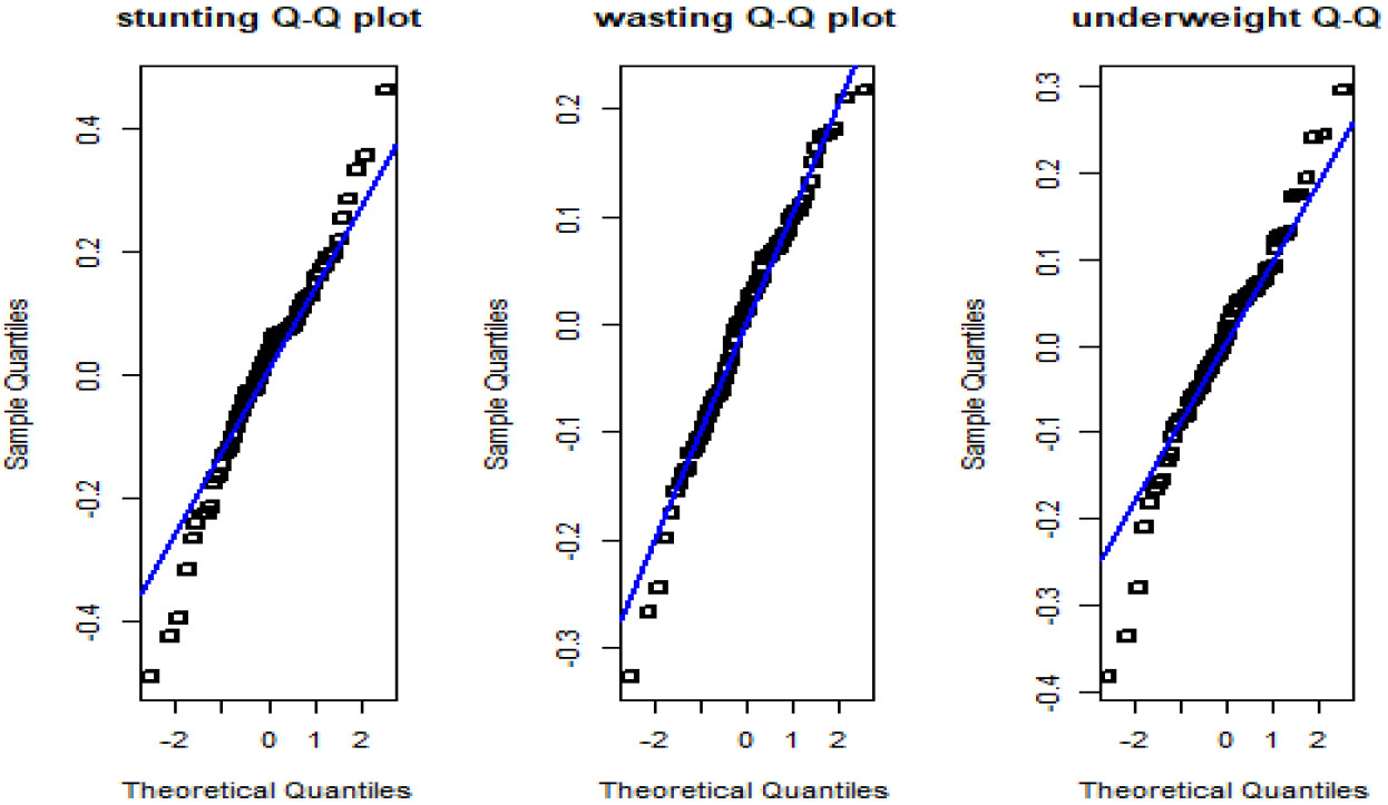
Figure 1.

Normal Q-Q plots of the residuals for stunting, wasting and underweight.

3.Results

3.1Variables selection and model comparison

This study took into account many auxiliary variables (approximately 41). On the other hand, the appropriate variables are chosen using principal component analysis (PCA), which reduces the number of variables to a few key components with minimal information loss [10]. PCA generates components that concentrate more explained variation in the first few principal components than any other variable in the original data. PCA uses an orthogonal transformation process to turn a set of observations of possibly correlated variables into a set of principal component values, which are uncorrelated variables. The number of primary components produced was 41, the same as the number of auxiliary variables. Nonetheless, the first eight principal components were kept (Table 1) since their eigenvalues were greater than one, and they explained 85.67 percent of the overall fluctuations [37].

Table 1

The first 8 principal components with eigenvalues

	Eigenvalue	Difference	Proportion	Prin (%)
1	16.23	9.57	0.3959	39.59
2	6.66	2.35	0.1624	55.83
3	4.31	1.91	0.1051	66.34
4	2.41	0.57	0.0587	72.20
5	1.83	0.29	0.0446	76.66
6	1.54	0.43	0.0376	80.42
7	1.11	0.06	0.0270	83.12
8	1.05	0.15	0.0255	85.67

In this result, we compared different multivariate Fay Herriot models to check the existence of correlations among target variables and the heteroscedasticity of covariance for random area effects. Accordingly, we equated the models using z scores of undernutrition to check the existence of correlations and to decide relatively the best model for further analysis. The estimates of the model variance component estimators (σ^ν1=0.0001, σ^ν2=0.0265, σ^ν3=0.0094 and ρ^=0.48) were first estimated under the heterogeneous model. The p values of the pairs of random zonal effects variance component estimators 0.58 for σ^ν12 and σ^ν22, 0.84 for σ^ν12 and σ^ν32, and 0.30 for σ^ν22 and σ^ν32 are insignificant at 5% levels of significance. Therefore, we can conclude that the zonal level random effects variances are homogeneous [2, 4]. Consequently, homogeneous MFH model is relatively better than the heteroscedastic model. In addition, the p value of test of correlation parameter (ρ) under homogeneous MFH model was zero. Hence, the multivariate Fay Herriot model with homogeneous variance is more likely the best model so we used this model for the rest of the analysis. The estimated model variance component parameters in this model are (σ^ν=0.013, ρ^=0.7638) which shows strong correlation between the target variables of stunting, wasting and underweight.

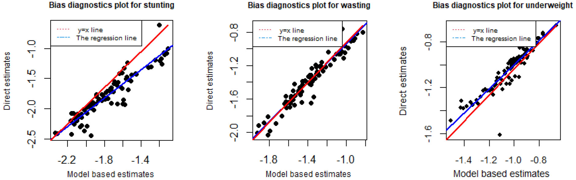
Figure 2.

Bias diagnostic plot with y=x line (red line) and regression line (blue line) for stunting, wasting and underweight for zones in Ethiopia: Model based MFH estimates versus direct estimates.

3.3The performance measures and improvements

The model diagnostics measures of small area estimates under the homogeneous variance MFH model are based on the arguments that model-based small area estimates should be consistent, unbiased, and more precise than direct survey estimates. The model-based small area estimates should provide an approximation to the direct survey estimates, so these values are consistent and close to the expected values of direct estimates. The small area estimates under the MFH model should have less variability than the corresponding direct survey estimates. The bias diagnostics, CV, and root MSE measures were performed in this research for the reliabilities, validities, and precisions of the model-based multivariate small area estimate for the three target variables.

The direct survey estimates on the y-axis vs. the model-based multivariate small area estimates on the x-axis are plotted (Fig. 2). The bias diagnostic plots in (Fig. 2) tested the argument that the deviation of the multivariate small area estimates regression line (blue line) from the line of equality y=x line (red line). These plots reveal that the multivariate small area estimates under the MFH model nearly converge with the survey estimates. These bias diagnostic measures indicated that the model based multivariate EBLUP is more likely to be consistent with direct survey estimates.

Furthermore, we can compute the Wald test statistic for the goodness of fit diagnostic. Following [38], the difference between the model-based estimates and the direct survey estimates should not be significant. The value of the Wald test statistic for the goodness of fit diagnostic follows χ2 square distribution with m=87 degree of freedom. The null hypothesis in this test is the EBLUP estimates didn’t differ significantly from the direct estimates. Consequently, the values of Wald test statistic is 30.2 with p-values = 1 for stunting, 23.4 with p-values = 1 for wasting and 44 with p-values = 0.99 for underweight. Therefore, there is not enough evidence to reject the null hypothesis implies that the model-based estimates and the direct estimates are statistically equivalent.

Table 2

Summary statistics of CV (%) for direct, UFH and MFH model estimates for the three target variables (the z scores of stunting, wasting and underweight)

Values	Sample sizes	Stunting			Wasting			Underweight
		Direct	UFH	MFH	Direct	UFH	MFH	Direct	UFH	MFH
Minimum	3	3.26	3.19	3.02	3.84	3.65	3.58	3.40	3.30	3.16
Q1	38	5.41	4.89	4.34	6.93	5.73	5.44	5.79	5.18	4.60
Median	78	7.57	6.42	5.28	9.54	7.60	6.66	8.53	6.77	5.79
Mean	97	9.45	6.80	5.55	11.37	7.88	6.98	9.54	6.79	6.14
Q3	126	11.16	7.98	6.35	13.47	9.61	7.81	10.91	8.00	7.20
Maximum	457	32.93	12.63	9.65	34.02	15.18	10.33	41.60	12.11	11.47

NB: all CV (%) are in absolute values.

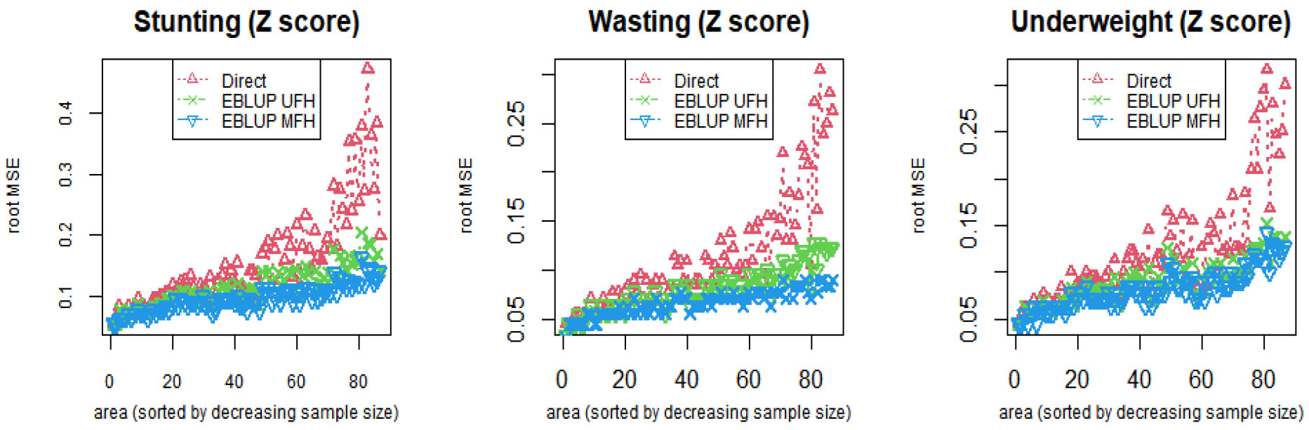
Figure 3.

Zones (sorted by decreasing sample size) root MSE’s of direct, EBLUP UFH and EBLUP MFH model estimates of stunting, wasting and underweight for children under age five.

A summary statistics of the CV (%) of the direct, univariate EBLUP and multivariate EBLUP of stunting, wasting, and underweight were presented in (Table 2). The CV (%) of the multivariate small area estimates (both UFH and MFH) is less than the direct survey estimates for all target variables. The CV (%) of direct survey estimates varied from 3.26 to 32.93 with a mean value of 9.45 for stunting, 3.84 to 34.02 with a mean value of 11.37 for wasting, and 3.40 to 41.60 with a mean value of 9.54 for underweight (Table 2). On the other hand, the CV (%) of univariate small area estimates under the UFH model ranged from 3.19 to 12.63 with a mean value of 6.80 for stunting, 3.65 to 15.18 with a mean value of 7.88 for wasting, and 3.30 to 12.11 with a mean value of 6.79 for underweight. In addition, the multivariate small area estimates of CV (%) were varied from 3.84 to 9.65 with a median value of 6.80 for stunting, 3.58 to 10.33 with a median value of 6.66 for wasting, and 3.16 to 11.47 with a median value of 5.79 for underweight in (Table 2). The summary statistics of the first and the third quartiles show that the CV (%) of the direct survey estimates are more than the model-based estimates (both in UFH and MFH models) in all target variables.

Figure 4.

Zones (sorted by decreasing sample size) CV (%) of direct, EBLUP UFH and EBLUP MFH estimators of stunting, wasting and underweight for children under age five.

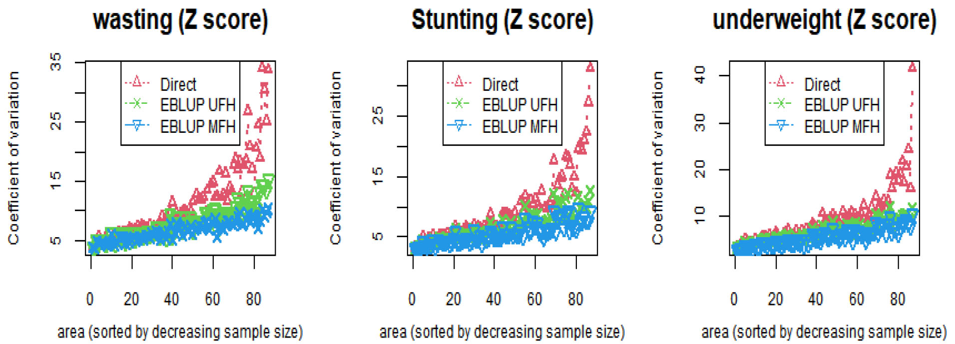
The root MSEs and the CV (%) of the direct survey estimate, univariate and multivariate EBLUPs of stunting, wasting, and underweight were reported in (Figs 3 and 4) respectively. In (Fig. 3), the zone-specific (with decreasing sample size) root MSE of multivariate small area estimates (blue) is smaller than the direct survey estimates (red) and the univariate small area estimates (green) for stunting, underweight, and wasting. The direct survey estimates have unacceptably high standard errors for all target variables as the sample size decreases (Fig. 3). However, the root MSE of the direct survey estimates are improved by model-based multivariate small area estimates due to the strong correlations among stunting, wasting, and underweight. Therefore, the results indicated that the direct survey estimates of all the three target variables are unstable (Table 2), (Fig. 3), and (Fig. 4). On the other hand, multivariate EBLUP with the smallest CVs is considered more reliable and precise estimates of undernutrition.

Table 3

Summary results of efficiency gain of MFH over UFH and direct survey estimates

	Efficiency gain MFH over Direct estimate			Efficiency gain MFH over UFH
Statistics	Stunting	Wasting	Underweight	Stunting	Wasting	Underweight
Minimum	6.89	4.48	5.94	3.87	-4.37	2.27
1st quartile	21.94	13.86	18.70	12.96	6.42	7.94
Median	30.63	19.82	25.77	17.32	10.77	9.69
Mean	33.44	23.66	28.43	17.05	12.72	9.53
3rd quartile	43.66	29.91	33.73	21.28	18.44	11.16
Maximum	72.14	57.99	72.42	29.93	36.49	16.72

Table 4

Summary statistics for small area estimation under MFH Model for non-sampled zones

Statistic	Direct			EBLUP			CV for direct estimate			CV for EBLUP
	Stunt	Wast	Under weight	Stunt	Wast	Under weight	Stunt	Wast	Under weight	Stunt	Wast	Under weight
Min	–	–	–	1.61	1.37	1.04	–	–	–	4.51	4.69	7.01
Q1	–	–	–	1.78	1.48	1.08	–	–	–	8.20	8.27	11.73
Mean	–	–	–	1.90	1.59	1.18	–	–	–	13.66	13.49	17.21
Q3	–	–	–	2.04	1.71	1.26	–	–	–	19.33	18.29	21.60
Max	–	–	–	2.09	1.73	1.43	–	–	–	23.28	23.13	29.45

The summary efficiency gain results for multivariate EBLUP estimates over the univariate EBLUP estimates, and the direct survey estimates were presented in (Table 3). The maximum efficiency gain for multivariate EBLUP over direct survey estimates was recorded 72.14 in Bahir Dar, 57.99 in Derashe special woreda, and 72.42 in Hawasa for stunting, wasting, and underweight, respectively. Similarly, the multivariate EBLUP over the univariate EBLUP was 29.93 for Bahir Dar, 39.49 for Huru guduru, Wollega, and 16.72 for Mao komo special zone for the target variables stunting, wasting, and underweight, respectively. The maximum improvements in efficiency have been recorded for zones with small sample sizes. For instance, Hawasa city and Bahir Dar city have the smallest sample sizes, 5 and 7, respectively. Whereas the minimum efficiency gain in CV was recorded for large sample sizes. The minimum efficiency gains in CV for multivariate over univariate small area estimates have been recorded: 3.87 in Korahe, -4.37 in Kemashe, and 2.27 in Derashe for stunting, wasting, and underweight. The negative minimum efficiency gain in CV for the Kemashe zone shows the loss of efficiencies for multivariate over univariate small area estimates [39]. Zones having relatively large sample sizes, have the minimum efficiency gain in CV. Therefore, the multivariate small area estimates didn’t improve the direct and univariate small area estimates for large sample sizes (Fig. 4). These results are relatively a good indicator that multivariate small area estimates were reliable for small sample sizes as the same time survey estimates are reliable for large sample sizes.

Table 4 reported the summary statistics of the non-sampled zones (zero sample size for each zone) under the MFH model for stunting wasting and underweight. There were eight non-sampled zones (Adama special zone, Amaro, Argoba, Basketo, Burayu, Fiq, Jimma special zone, and Konso special woreda) under 2016 Ethiopian DHS. Small area estimate is the optimum approach for non-sampled zones or zones with zero sample sizes [32]. The small area estimates and CV (%) of stunting, wasting, and underweight were estimated based on the MFH model for non-sampled zones using auxiliary covariates from the census (Table 4). We cannot establish a comparison of CV for non-sampled zones since there are no direct survey estimates for them. The small area estimates and the CV of the non-sampled zones, on the other hand, are consistent with the results of the sampled zones.

4.Discussion

The target variables of the study were obtained from the 2016 Ethiopian demographic and health survey (EDHS), and the auxiliary variables are taken from the 2007 population and housing census data. Principal component analysis was used to reduce the number of auxiliary variables to a few informative variables. Unlike the survey study by [16, 40], this study was the small area estimations of unplanned domains with small sample sizes for the correlated target variables by borrowing strength from the census data. In contrast to the univariate FH model, which ignores the correlation among the target variables [41, 42, 43], this study considered the correlations among three target variables for a small sample size. Following the correlations of the target variables, the univariate model becomes the MFH model [7, 8, 11]. We considered three particularizations of the model in [7] to detect the existence or nonexistence of a correlation and heteroscedasticity. Likewise, we discussed the three models in detail, and the homogeneous variance MFH model was considered appropriate.

The normality assumption of the selected model is valid via the Shapiro-Wilk test and normal Q-Q plot. The Q-Q plots and the Shapiro-Wilk test have concluded that the sampling errors are expected to be normally distributed [10, 11]. The bias diagnostic measures and the Wald test statistic for the goodness of fit indicated that the model-based multivariate small area estimates are likely to be consistent with the direct survey estimates for all target variables. These diagnosis checking were coherently agreed with the previous studies [10, 11, 12, 38].

The performance measures of the multivariate EBLUP over the univariate small area estimates and the direct survey estimates were measured by CV and root MSE [7, 8, 9]. The direct survey estimates of the target variables (stunting, wasting, and underweight) had the largest variabilities with small sample sizes. The root MSE of the direct survey estimates were more than the corresponding model-based multivariate EBLUP [7]. This is because of considering the correlation between related target variables of interest in the model-based multivariate EBLUP estimates [10].

The best efficiency gains were recorded for the model-based multivariate EBLUPs over the direct survey estimates in all zones for small sample sizes. The Multivariate EBLUP improved the univariate small area estimates and direct estimates. These improvements were obtained because of the correlations of the target variables [10]. Thus, multivariate EBLUP under the MFH model is the best reliable, efficient, and precise for all target variables stunting, wasting, and underweight [8, 10, 44, 45]. Multivariate small area estimates improve the univariate small area estimates and direct survey estimates due to the correlations among the target variables. The summary statistics of the non-sampled zones for all target variables were produced under the MFH model [1, 5, 32, 36]. The estimation of non-sampled zones under the MFH model is precise and adequate with similar approaches to the results of sampled zones [32]. The availability of reliable and adequate estimates of non-sampled zones will help the government give them equal attention to 87 sampled zones.

5.Conclusions

This study applied the MFH models using the 2016 survey by linking with 2007 population and housing census data. Under the three MFH models, the homogeneous variance MFH model is appropriate to obtain relatively reliable, efficient, and precise estimates. The model diagnostic measures directed that the model-based multivariate small area estimates are reliable to the direct survey estimates. Furthermore, the MFH model’s sampling errors are normally distributed for all target variables. The CV and the root MSE indicated that the model-based multivariate small area estimations are the most reliable, efficient, and precise under the homogeneous MFH model. The performance measures of CV and root MSE under the MFH model provided a significant gain in efficiency to obtain zonal level estimates of stunting, wasting, and underweight. The direct survey estimates are some high standard errors with small sample sizes, but these high standard errors are reduced by using multivariate small area estimates. Multivariate small area estimates highly improve the direct survey estimates because they have significant correlations between stunting, wasting and underweight.

In Ethiopia, surveys are planned to produce national and regional level estimates, while zonal levels are not considered in the survey. However, zones are an essential domain for the planning and monitoring process, and therefore the availability of zonal level statistics plays a prominent role for planning and policymakers. This study has produced the best reliable, efficient, and precise statistics with sampled and non-sampled zones and provides valuable information to policymakers, planners, and legislative organs of the government. One of the novelties of this paper is estimating the non-sampled zones, and therefore the policymakers will give equal attention similar to the sampled zones.

References

[1] | Rao JNK, Molina I. Small area estimation. 2nd ed. Hoboken: (2015) . |
[2] | Fay RE, Herriot RA. Estimates of income for small places: an application of james-stein procedures to census data. J Am Stat Assoc (1979) ; 74: : 269-77. doi: 10.1080/01621459.1979.10482505. |
[3] | Datta GS, Rao JNK, Smith DD. On measuring the variability of small area estimators under a basic area level model. Biometrika Trust (2005) ; 92: : 183-96. |
[4] | Shiferaw Y, Galpin J. A corrected confidence interval for a small area parameter through the weighted estimator under the basic area level model. J Iran Stat Soc. (2019) ; 18: : 17-51. doi: 10.29252/jirss.18.1.17.A. |
[5] | Shiferaw Y, Galpin J. Improved Confidence Intervals for a Small Area Mean Under The Fay-Herriot Model. University of the Witwatersrand, (2016) . |
[6] | Fay RE. Application of multivariate regression to small domain estimation. Small Area Stat (1987) ; 91-102. |
[7] | Benavent R, Morales D. Multivariate Fay-Herriot models for small area estimation. Comput Stat Data Anal. (2016) ; 94: : 372-90. doi: 10.1016/j.csda.2015.07.013. |
[8] | Ubaidillah A, Notodiputro KA, Kurnia A, Mangku IW. Multivariate Fay-Herriot models for small area estimation with application to household consumption per capita expenditure in Indonesia. J Appl Stat. (2019) ; 46: : 2845-61. doi: 10.1080/02664763.2019.1615420. |
[9] | Guha S, Chandra H. Measuring disaggregate level food insecurity via multivariate small area modelling: evidence from rural districts of Uttar Pradesh, India. Food Secur. (2021) ; 13: : 597-615. doi: 10.1007/s12571-021-01143-1. |
[10] | Guha S, Chandra H. Measuring and mapping disaggregate level disparities in food consumption and nutritional status via multivariate small area modelling. Soc Indic Res. (2021) ; 154: : 623-46. doi: 10.1007/s11205-020-02573-8. |
[11] | Moretti A, Shlomo N, Sakshaug JW. Multivariate small area estimation of multidimensional latent economic well-being indicators. Int Stat Rev. (2019) ; 88: : 1-28. doi: 10.1111/insr.12333. |
[12] | Moretti A, Shlomo N, Sakshaug JW. Parametric bootstrap mean squared error of a small area multivariate EBLUP. Commun Stat Simul Comput. (2018) ; 49: : 1474-86. doi: 10.1080/03610918.2018.1498889. |
[13] | Ito T, Kubokawa T. On measuring the variability of small area estimators in a multivariate fay-herriot model. (2018) : 1-21. |
[14] | Muller O, Krawinkel M. Malnutrition and health in developing countries. Cmaj. (2005) ; 173: : 279-86. |
[15] | UNICEF, WHO, World Bank. Levels and trends in child malnutrition: Key findings of the 2020 Edition of the Joint Child Malnutrition Estimates. Geneva WHO. (2020) ; 24: : 1-16. |
[16] | Tekile AK, Woya AA, Basha GW. Prevalence of malnutrition and associated factors among under-five children in Ethiopia: evidence from the 2016 Ethiopia Demographic and Health Survey. BMC Res Notes. (2019) ; 12: : 1-6. doi: 10.1186/s13104-019-4444-4. |
[17] | CSA, ICF. Ethiopia Demographic Health Survey. Addis Ababa, Ethiopia, and Rockville, Maryland, USA: CSA and ICF, (2016) . |
[18] | De Onis M. WHO child growth standards. (2006) . |
[19] | Amare D, Negesse A, Tsegaye B, Assefa B, Ayenie B. Prevalence of undernutrition and its associated factors among children below five years of age in Bure Town, West Gojjam Zone, Amhara National Regional State, Northwest Ethiopia. Adv Public Heal. (2016) ; 2016: : 8. doi: 10.1155/2016/7145708. |
[20] | Endris N, Asefa H, Dube L. Prevalence of malnutrition and associated factors among children in rural Ethiopia. Biomed Res Int. (2017) ; 2017: : 6. doi: 10.1155/2017/6587853. |
[21] | Gebre A, Reddy PS, Mulugeta A, Sedik Y, Kahssay M. Prevalence of malnutrition and associated factors among under-five children in pastoral communities of Afar Regional State, Northeast Ethiopia: a community-based cross-sectional study. J Nutr Metab. (2019) ; 2019: : 13. doi: 10.1155/2019/9187609. |
[22] | Tadesse S, Alemu Y. Urban-rural differentials in child undernutrition in Ethiopia. Int J Nutr Metab. (2015) ; 7: : 15-23. doi: 10.5897/IJNAM2014.0171. |
[23] | Woodruff BA, Wirth JP, Bailes A, Matji J, Timmer A, Rohner F. Determinants of stunting reduction in Ethiopia 2000–2011. Matern Child Nutr. (2017) ; 13: . doi: 10.1111/mcn.12307. |
[24] | Yeshaw Y, Kebede SA, Liyew AM, Tesema GA, Agegnehu CD, Teshale AB, et al. Determinants of overweight/obesity among reproductive age group women in Ethiopia: multilevel analysis of Ethiopian demographic and health survey. BMJ Open. (2020) ; 10: : e034963. doi: 10.1136/bmjopen-2019-034963. |
[25] | Fenta HM, Zewotir T, Muluneh EK. Spatial data analysis of malnutrition among children under-five years in Ethiopia. BMC Med Res Methodol. (2021) ; 21: : 1-13. doi: 10.1186/s12874-021-01391-x. |
[26] | Fenta HM, Zewotir T, Muluneh EK. A machine learning classifier approach for identifying the determinants of under – five child undernutrition in Ethiopian administrative zones. BMC Med Inform Decis Mak. (2021) ; 21: : 1-12. doi: 10.1186/s12911-021-01652-1. |
[27] | Fenta HM, Zewotir T, Muluneh EK. Disparities in childhood composite index of anthropometric failure prevalence and determinants across Ethiopian administrative zones. PLoS One. (2021) ; 16: : 1-17. doi: 10.1371/journal.pone.0256726. |
[28] | Woldie M, Jirra C, Azene G. Presence and use of legislative guidelines for the distribution of decentralized decision making authority in the Jimma zone health system, Southwest Ethiopia. Ethiop J Health Sci. (2011) ; 21: : 29. |
[29] | Kitaw Y, Teka G-E, Meche H, Damen H, Fentahun M. The evolution of public health in Ethiopia. 2nd ed. (2012) . |
[30] | Klaver W. Underweight or stunting as an indicator of the MDG on poverty and hunger. (2010) . |
[31] | Chubb H, Simpson JM. The use of Z-scores in paediatric cardiology. Ann Pediatr Cardiol. (2012) ; 5: . doi: 10.4103/0974-2069.99622. |
[32] | Chandra H. Exploring spatial dependence in area-level random effect model for disaggregate-level crop yield estimation. J Appl Stat. (2013) ; 40: : 823-42. doi: 10.1080/02664763.2012.756858. |
[33] | CSA. Federal Democratic Republic of Ethiopia Central Statistical Agency Population Projection of Ethiopia for All Regions At Wereda Level from 2014–2017. (2013) . |
[34] | Gizaw Z, Woldu W, Bitew BD. Acute malnutrition among children aged 6–59 months of the nomadic population in Hadaleala district, Afar region, northeast Ethiopia. Ital J Pediatr. (2018) ; 44: : 1-10. doi: 10.1186/s13052-018-0457-1. |
[35] | Wirth JP, Rohner F, Petry N, Onyango AW, Matji J, Bailes A, et al. Assessment of the WHO Stunting Framework using Ethiopia as a case study. Matern Child Nutr. (2017) ; 13: : e12310. doi: 10.1111/mcn.12310. |
[36] | Permatasari N, Ubaidillah A. Msae: An R Package of Multivariate Fay Herriot Models for Small Area Estimation. R J (2021) ; 1-12. |
[37] | Warnholz S. Small area estimation using robust estenstions to area level models theory, implementation and simulation studies. Freie Universität Berlin, (2016) . |
[38] | Mukhopadhyay PK, McDowell A. Small area estimation for survey data analysis using SAS software. SAS Glob. Forum, vol. 2011, (2011) , p. 96. |
[39] | Ogwu MC, Osawaru M. Principal component analysis: A tool for multivariate analysis of genetic variability. African J Plant Sci. (2016) . |
[40] | Brown G, Chambers R, Heady P, Heasman D. Evaluation of small area estimation methods – an application to unemployement estimats from the UK LFS. Proc. Stat. Canada Symp. (2001) ; pp. 1-10. doi: 10.1201/9780203166314.ch1. |
[41] | Li H. Small Area Estimation: An Empirical Best Linear Unbiased Prediction Approach. University of Maryland, (2007) . |
[42] | Rajkumar AS, Gaukler C, Tilahun J. Combating Malnutrition in Ethiopia: An Evidence-Based Approach for Sustained Results: World Bank Publications. (2012) . doi: 10.1596/978-0-8213-8765-8. |
[43] | Rao J. Small-area estimation. Wiley StatsRef Stat Ref Online. (2014) ; 1-8. doi: 10.1002/9781118445112.stat03310.pub2. |
[44] | Datta GS. Model-based approach to small area estimation. Sample Surv Inference Anal. (2009) ; 29B: : 251-88. doi: 10.1016/S0169-7161(09)00232-6. |
[45] | Islam S, Chandra H. Small area estimation combining data from two surveys. Commun Stat Comput. (2019) ; 36: : 1-22. doi: 10.1080/03610918.2019.1588308. |
[46] | Islam S, Chandra H, Aditya K, Lal SB. Small area estimation under a spatial model using data from two surveys. Int J Agric Stat Sci. (2018) ; 14: : 231-7. |
[47] | Esteban MD, Morales D, Pérez A, Santamaría L. Area-level time models for small area estimation of poverty indicators. Comb Soft Comput Stats Methods. (2010) ; 77: : 233-7. doi: 10.1007/978-3-642-14746-3_29. |