
Assessment of the spread of COVID-19 in seven countries using a seasonal adjustment method
Abstract
Early identification of the trends in the number of newly confirmed COVID-19 cases is essential. Weekly periodicity and irregular fluctuations affect the time series of the number of newly confirmed COVID-19 cases. However, a 7-day moving average and a rolling 7-day total delay identifying the trend changes because of assigning a low weight to the most recent day. Additionally, they cannot adjust for the fluctuations due to moving holidays.
For the first time, this study shows that X-13ARIMA-SEATS (X-13), one of the seasonal adjustment methods, can apply to the analysis of the changes in the number of newly confirmed COVID-19 cases with examples of seven countries: Germany, Indonesia, Iran, Russia, the United Kingdom, the United States, and Japan.
This study successfully extracts trend components, calendar-induced components (weekly periodicity and fluctuations due to moving holidays), and irregular components from the time series of seven countries by X-13. Thus, compared to a 7-day moving average and a rolling 7-day total, the method in this study can facilitate more rapid and accurate assessment and strategic responses to the spread of COVID-19. Furthermore, the method could be effective for analyzing other daily data with weekly periodicity.
Figure 1.
Flowchart of X-13 processes in this study.
1.Introduction
For national and local governments, early identification of the trends in the number of newly confirmed COVID-19 cases is essential for rolling out prompt strategic responses. Therefore, they count the number of newly confirmed COVID-19 cases daily.
Weekly periodicity and irregular fluctuations usually affect the time series of newly confirmed COVID-19 cases. Therefore, a substantial number of national and local governments use a 7-day moving average or a rolling 7-day total to track the trends in the number of newly confirmed COVID-19 cases [1, 2]. However, the 7-day moving average and the rolling 7-day delay identifying the trend changes because of assigning a low weight, 1/7, to the most recent day. Additionally, they cannot adjust for the fluctuations due to moving holidays.
This study applies X-13ARIMA-SEATS (X-13) to analyze the number of newly confirmed COVID-19 cases in seven countries to resolve these challenges. X-13 is one of the seasonal adjustment methods developed by the U.S. Census Bureau and widely used in economic statistics. However, X-13 can apply to only quarterly or monthly data. Hence, this study modifies one of the subprograms in X-13 to apply daily data with weekly periodicity.
In the first place, Section 2, ‘Methodology,’ outlines the overview of X-13 processes in this study and the modified subprogram in X-13. Then, Section 3, ‘Result,’ presents trend components, calendar-induced components (weekly periodicity and fluctuations due to moving holidays), and irregular components (irregular fluctuations) extracted from the number of newly confirmed COVID-19 cases by X-13. Finally, Section 4, ‘Discussion,’ provides some discussion of the method and analysis in this study.
2.Methodology
2.1Seasonal adjustment method used in this study
X-13, TRAMO/SEATS, and Seasonal-Trend decomposition using LOESS (STL) are seasonal adjustment methods. X-13 and TRAMO/SEATS can apply to only quarterly or monthly data. Nevertheless, they are common in economic statistics. STL can apply to daily data, although determining the smoothing parameters is complex [3]. The program of X-13 requires dealing with the challenge of not being able to handle daily data. Nevertheless, this study selects X-13 because it involves a simple procedure.
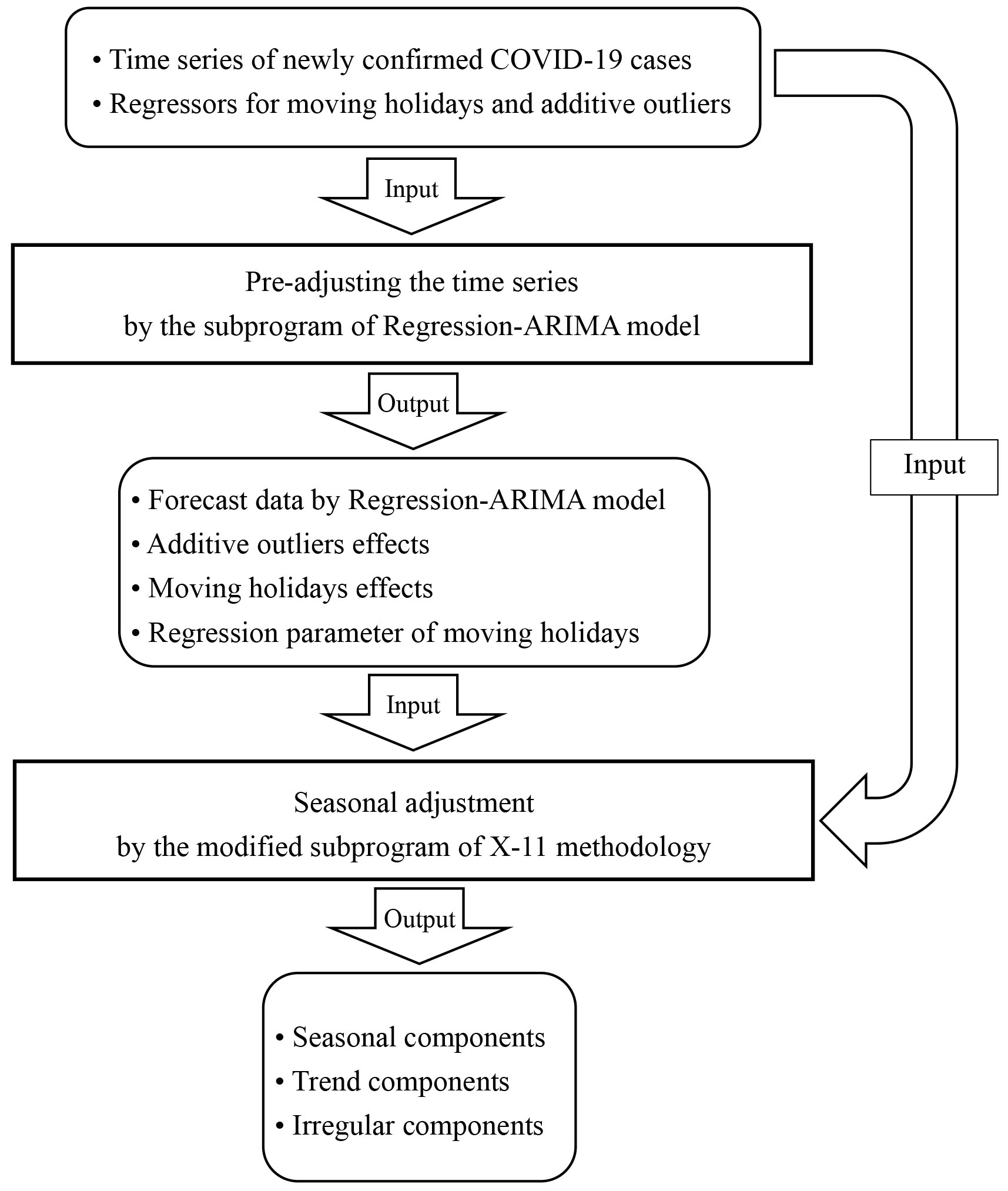
X-13 consists of two subprograms: pre-adjusting a time series (Forecasts, Backcasts, and Pre-adjustments) by the Regression-ARIMA model and seasonal adjustment by the X-11 methodology [4]. Figure 1 illustrates the flowchart of X-13 processes in this study.
Figure 2.
Flowchart of the modified subprogram of X-11 methodology in this study.
The Regression-ARIMA model is the following formula [5].
(1)
where
The Regression-ARIMA model can apply to daily data with weekly periodicity because the Regression-ARIMA model does not limit quarterly or monthly data. Therefore, this study does not modify the subprogram of the Regression-ARIMA model.
On the other hand, the X-11 methodology in X-13 contains some processes that assume quarterly or monthly data. Hence, this study modifies the subprogram of the X-11 methodology to apply to daily data with weekly periodicity. ‘2.2 The X-11 methodology’ describes the modifications of the subprogram and the flow of the seasonal adjustment process based on the modified subprogram.
2.2The X-11 methodology
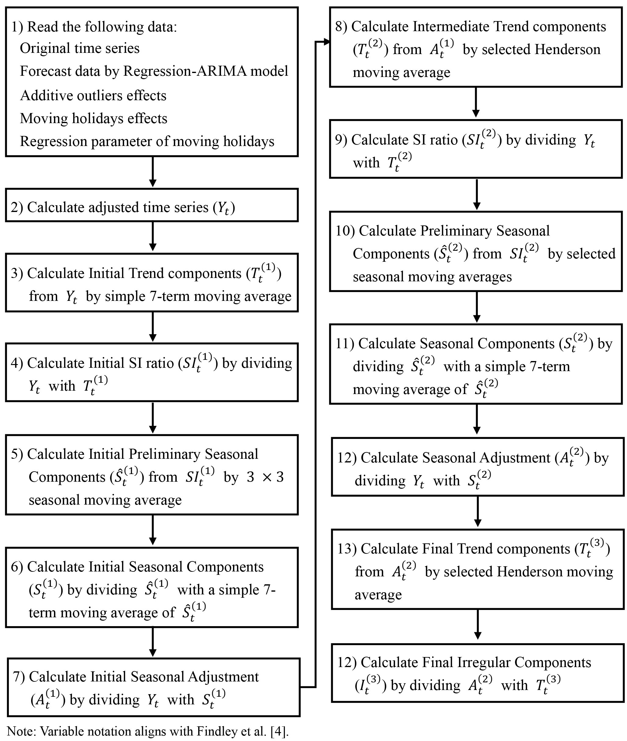
The X-11 methodology in X-13 is a procedure that decomposes a time series into trend components, seasonal components, and irregular components. This study modifies the subprogram of the X-11 methodology to apply to daily data with weekly periodicity by referring to Findley et al. [4], Dagum [6], and Tiller et al. [7].
Figure 2 illustrates the flowchart of the modified subprogram. It is 3), 5), 6), 10), and 11) in Fig. 2 that this study changes to apply to daily data with weekly periodicity.
2.3Three primary filters in the X-11 methodology
This section describes three primary filters in the X-11 methodology: moving averages, the Henderson filter (moving averages to extract trend components from seasonally adjusted series), and the seasonal filter (seasonal moving averages).
2.3.1Moving averages
Moving averages are a filter that extracts trend components from a time series. This study replaces the centered 4-term (for quarterly time series) and the centered 12-term (for monthly time series) moving averages with a simple 7-term moving average. The formulas of moving averages before and after the replacement are as follows:
(i) moving averages before the replacement
(ii) moving average after the replacement
where
The 7-term moving average keeps the formula to obtain the average for the seasonal period. Therefore, it can eliminate seasonal components of daily data with weekly periodicity. Additionally, the 7-term moving average (
2.3.2The Henderson filters
The Henderson filter extracts trend components from a time series consisting of only trend and irregular components. As the Henderson filter, the X-11 methodology employs weighted moving averages, called Henderson moving averages. Henderson moving averages are optimized to reproduce third-order polynomial. The X-11 methodology utilizes 9, 13, and 23-term Henderson moving averages for monthly data and 5- and 7-term Henderson moving averages for quarterly data [5]. The formula of Henderson moving averages is as follows [4]:
where
The formula of Henderson moving averages shows that it does not contain the seasonal period. Therefore, this study does not modify the formula. Therefore, this study utilizes the same Henderson moving averages of the X-11 methodology for monthly data.
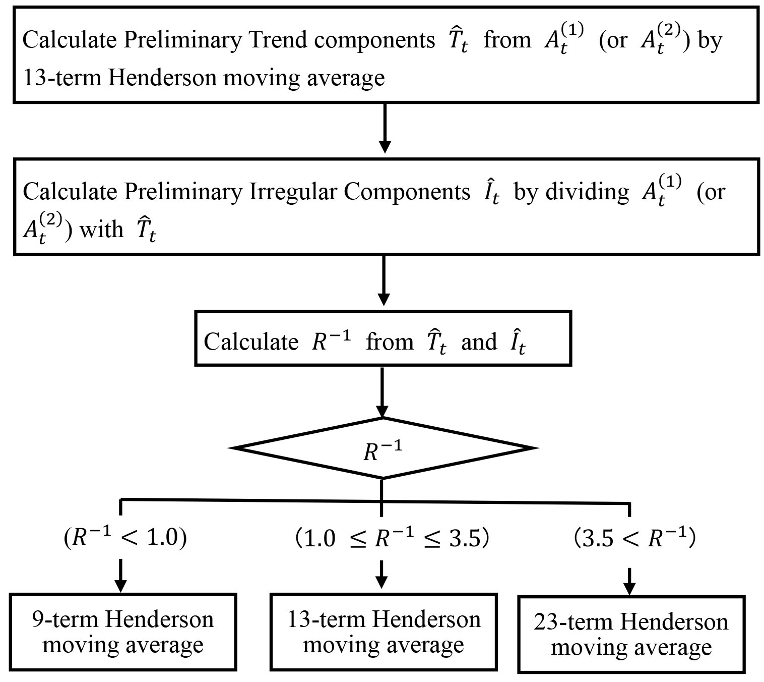
The X-11 methodology defines the term of Henderson moving averages by the I-bar C-bar ratio. The sample mean of absolute irregular components changes and absolute trend components changes determine the I-bar C-bar ratio. The formula of the I-bar C-bar ratio is as follow [4, 6]:
where
The formula of the I-bar C-bar ratio does not contain the seasonal period. Therefore, this study employs the same processes as the X-11 methodology to define the term of Henderson moving averages. Figure 3 illustrates the flowchart to define the term of Henderson moving averages in this study.
Figure 3.
Flowchart to define the term of Henderson moving averages.
2.3.3Seasonal filters
The seasonal filter extracts seasonal components from a time series consisting of only seasonal and irregular components. As a seasonal filter, the X-11 methodology employs
The X-11 methodology utilizes
(i) seasonal moving averages for monthly data (before the modification)
(ii) seasonal moving averages for daily time series with weekly periodicity
The modified seasonal moving averages keep the formulas that each interval of terms is the seasonal period. Therefore, they can extract seasonal components. Besides, the modification does not change the number of terms. Hence, the modified formulas expect to be the same capability to eliminate irregular components.
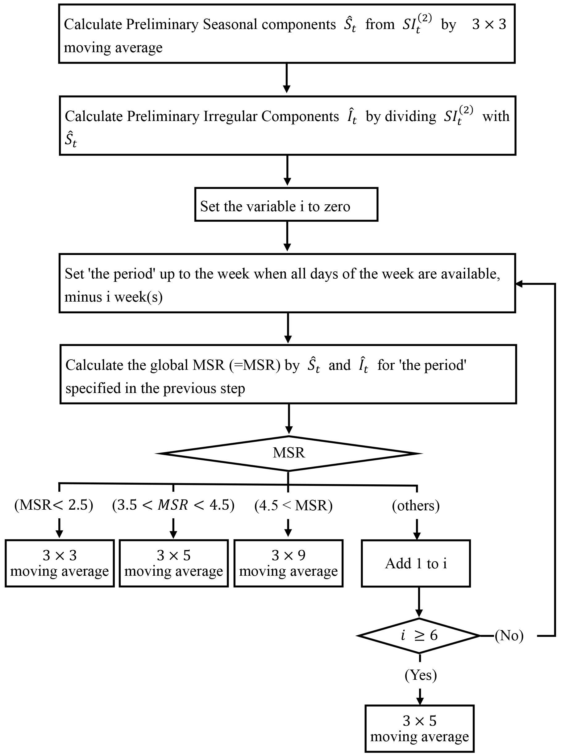
In the X-11 methodology, the moving seasonality ratio (MSR) procedure selects one of
(i) the global MSR ratio for monthly data (before the modification)
where
(ii) the global MSR ratio for daily data with weekly periodicity
where
This study employs the MSR procedure with the modified global MSR ratio to define the seasonal moving average. Figure 4 illustrates the flowchart to define the kind of seasonal moving average.
Figure 4.
Flowchart to define the kind of seasonal moving average.
2.4Data
This study obtains the number of newly confirmed COVID-19 cases in Germany, Indonesia, Iran, Russia, the United Kingdom, the United States of America, and Japan by the dataset of Johns Hopkins University from “Our World in Data” [9, 10]. The data period is from March 22, 2020, to July 2, 2021. This study treats faulty values (zero and negative values) as values of 0.1.
Figure 5.
Spectrum of original time series.
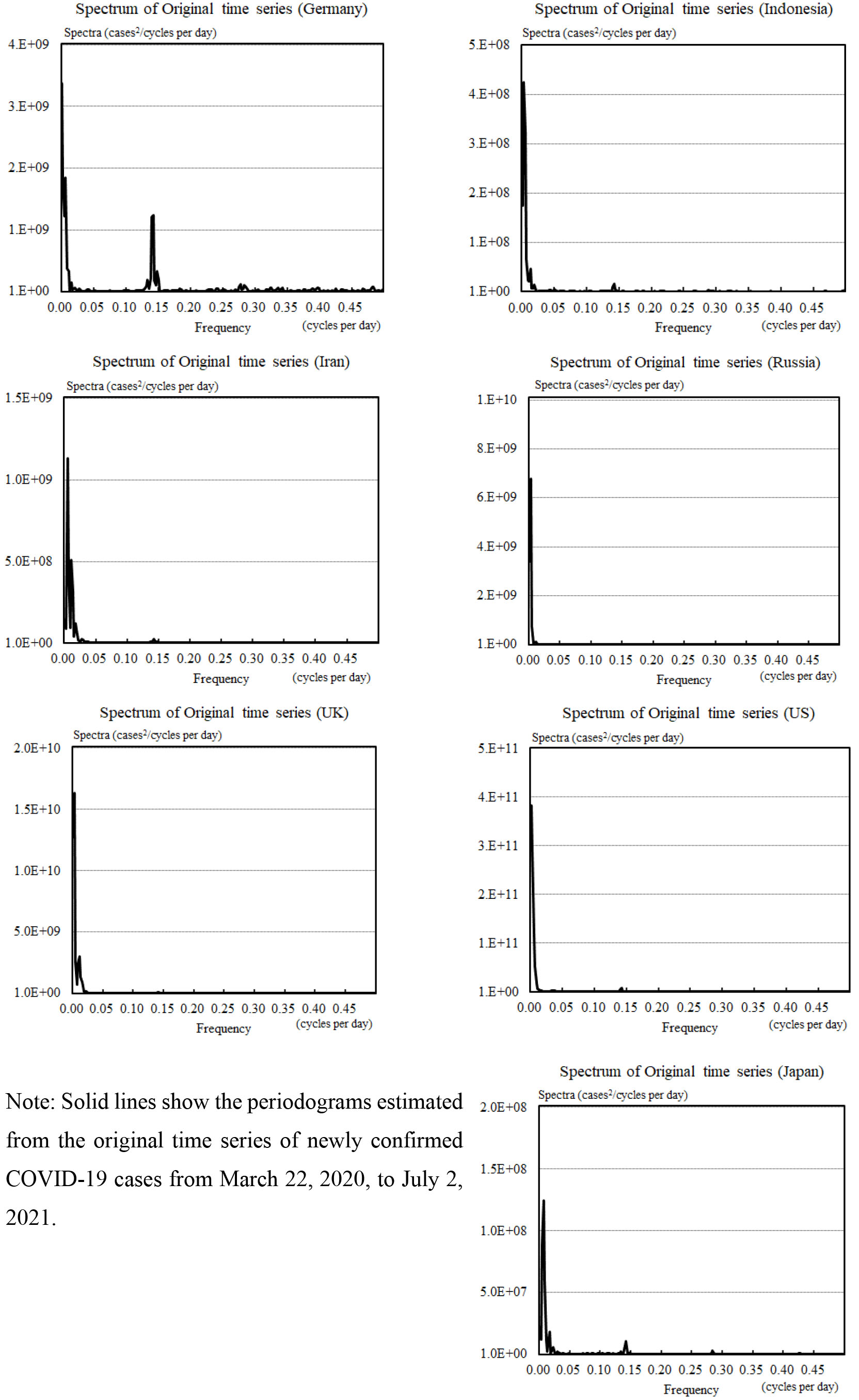
Figure 5 illustrates the periodograms estimated from the original time series of newly confirmed COVID-19 cases. Firstly, spectra of long-period (480, 240, or 120 days) are large in all 7 countries. Besides, spectra of weekly exist although the spectra are smaller than that of long-period. One main issue of this study can be expressed as extracting long-term, weekly-term, and short-term changes from the data of newly confirmed COVID-19 cases.
Table 1
Details of the estimated Regression-ARIMA models
| Country | ARIMA | Regressors | |
|---|---|---|---|
| model | Moving holiday | Additive outliers | |
| Germany | (0 1 1)(1 1 1) | x | (2020) 14 and 21 Apr./ 4, 14, 18, 19, 26, 28 and 29 May/ 6, 10, 11, 13, 15, 18, 21, 23 and 26 Jun./ 5, 6, 18 and 27 Jul./ 2 Aug./ 22 Oct./ 2, 3, 4, 9, 15, 22, 24, 25 and 29 Nov./ 5, 7, 14, 20, 25 and 30 Dec. (2021) 1, 7, 9, 10, 12, 15, 20, 21 30 and 31 Jan./ 9, 11, 17, 21 and 28 Mar./ 3, 6, 11 and 18 Apr./ 1, 9, 12, 25 and 26 May/ 6 Jun. |
| Indonesia | (3 1 1)(2 1 1) | x | (2020) 27 and 29 Mar./ 2, 4, 10, 12, 20, 27 and 29 Apr./ 11 and 23 May/ 9 and 29 Jul./ 3 Dec. (2021) 22 Feb./ 11 and 13 Mar./ 4 Apr./ 13 Jun. |
| Iran | (1 1 0)(0 1 1) | NA | (2020) 22, 23, 24 and 29 Mar./9, 23 and 27 Apr./ 2, 3, 6, 10, 12, 15, 18, 23, 26 and 29 May/ 4 and 7 Jun./ 9 and 10 Jul./ 10, 14 and 17 Sep./ 13, 22, 26 and 29 Oct./ 7 and 10 Nov. (2021) 31 Mar./ 5, 14, 15 May/ 2, 6, 7, 8, 10, 12 and 15 Jun. |
| Russia | (1 1 1)(1 1 1) | NA | (2020) 24, 25, 26, 27 and 31 Mar./ 1, 2, 4, 5, 11, 12, 15, 19, 20, 23 and 29 Apr./ 5, 11, 15, 16 and 24 May/ 6, 15 and 23 Oct./ 4, Nov. (2021) 5, 6 and 24, Jan./ 24 Feb./ 15 Mar./ 29 Apr./ 6, 14, 17 and 31 May/ 13, 16 and 17 Jun. |
| United Kingdom | (2 1 2)(1 1 1) | x | (2020) 28 and 30 Jun./1, 2, 6 and 14 Jul./ 3, 9, 11, 14, 17, 19 and 22 Aug./ 14 and 28 Sep./ 3 and 4 Oct./ 1, 12 and 24 Nov./ 6 and 20 Dec. (2021) 22 Feb./ 19 and 27 Mar./ 9 and 12 Apr./ 18 May |
| United States | (0 1 2)(0 1 1) | x | (2020) 1 Apr./ 8 and 21 Sep./ 19 Oct./ 1, 3 and 26 Nov./ 25 Dec. (2021) 1 and 2 Jan./ 24 Mar./ 4 Apr./ 31 May/ 1, 4, 5 and 17 Jun. |
| Japan | (1 1 0)(1 1 1) | x | (2020) 30 Mar./ 12, 14, 17, 19, 24, 28 and 29 May/ 3, 9, 12, 14 and 15 Jun./ 3, 8, 15, 16, 20 and 31 Jul./ 23 Sep. (2021) 6 and 7 Mar./ 28 Apr. |
Note: T-statistics for all ARIMA model parameters, regressors for moving holidays (except for Iran and Russia), and additive outliers are more significant than 2.6, meaning all the ARIMA model parameters and additive outliers have a significance level of 1%.
This study creates the regressors, which enable to separate fluctuations due to moving holidays, by the following steps:
(i) Create two new series, one series with ‘1’ for moving holidays and ‘0’ for the other days, and the other series with ‘1’ for the days after the moving holidays and ‘0’ for the other days. Preparing two series is that the fluctuations due to moving holidays may arise one day delayed.
(ii) Calculate the average of the series for each day of the week.
(iii) Subtract the average for each day of the week from the series to eliminate weekly periodicity.
(iv) If t-statistics is more than 2.6, the series is a regressor in Regression ARIMA-model.
3.Result
3.1Regression-ARIMA models
Table 1 presents the details of the estimated Regre-ssion-ARIMA models by the time series of seven countries. As a matter to note is there are no significant fluctuations due to moving holidays in Russia and Iran.
Table 2
Result of the QS statistics test
| QS statistic | ||
|---|---|---|
| Germany | 430.60 | 0.0000 |
| Indonesia | 50.69 | 0.0000 |
| Iran | 494.57 | 0.0000 |
| Russia | 249.48 | 0.0000 |
| United Kingdom | 71.69 | 0.0000 |
| United States | 213.07 | 0.0000 |
| Japan | 371.77 | 0.0000 |
Note: QS test is a statistical test for the hypothesis of no seasonality (
Table 2 illustrates the result of the QS statistics tests. The QS statistics test verifies the presence of weekly periodicity in a time series [5]. The result demonstrates that the likelihood of no weekly periodicity in any countries’ time series is very low.
Figure 6.
Trend components and original time series.
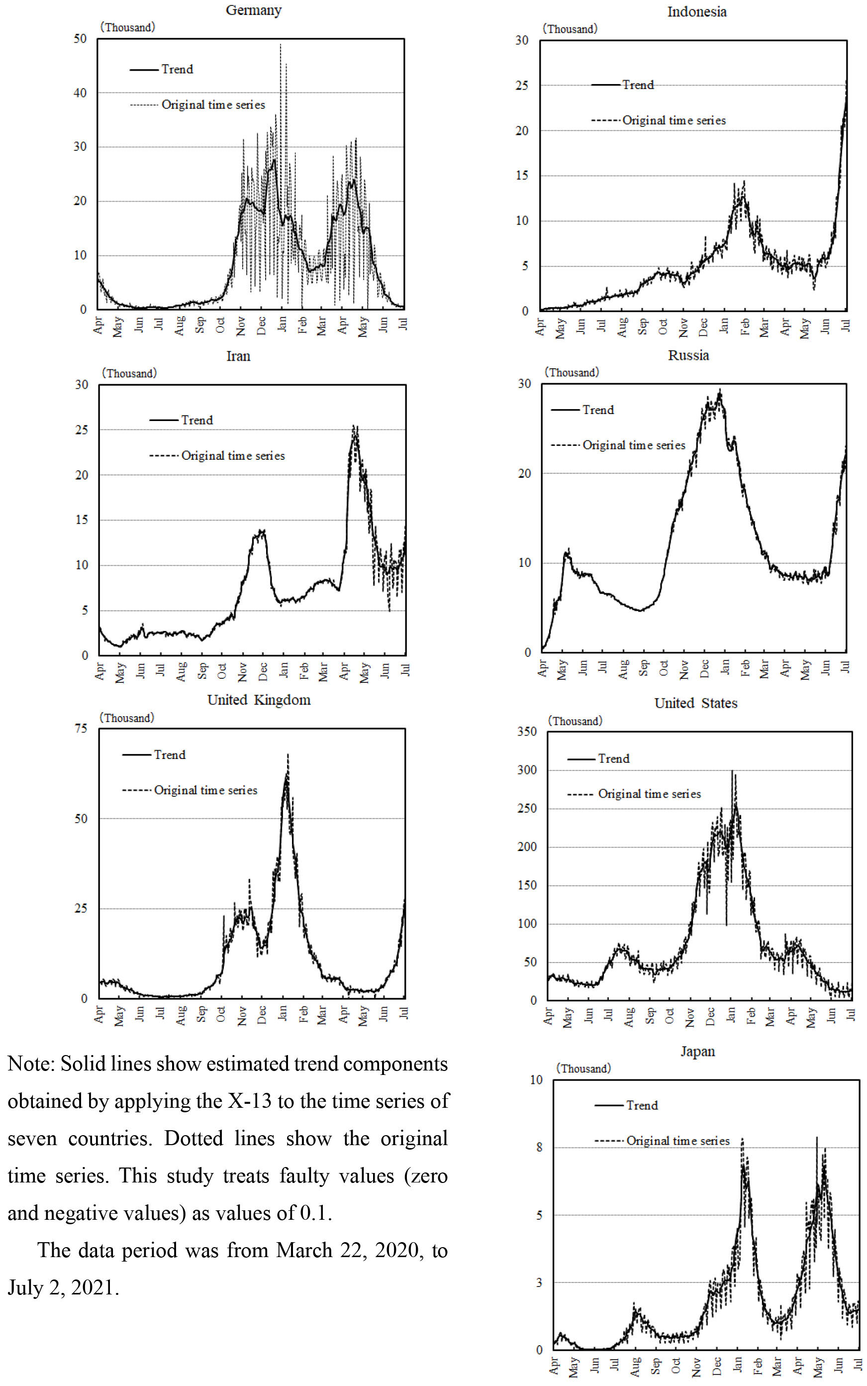
3.2Trend components
Figure 6 illustrates the estimated trend components in the number of newly confirmed COVID-19 cases. Moreover, Fig. 7 illustrates the periodograms estimated from the trend components. These figures show that the method in this study successfully extracts trend components as a long-term variation.
Figure 7.
Spectrum of trend components.
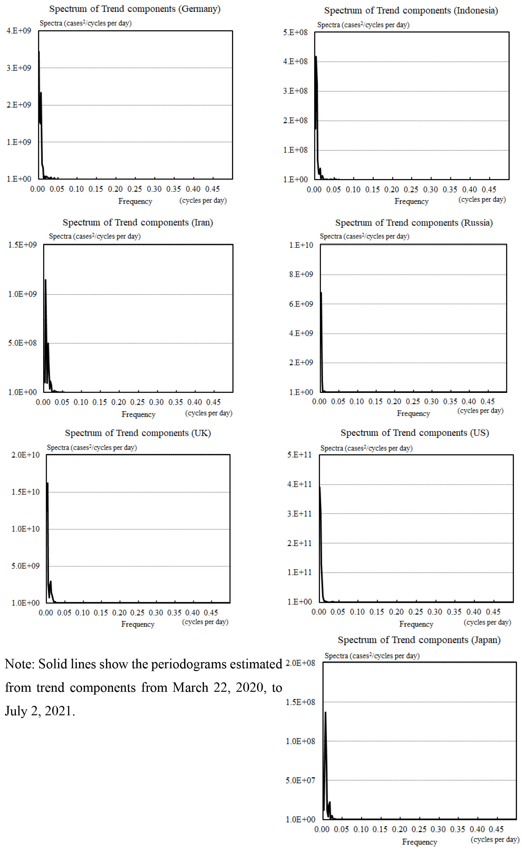
Figure 8.
Frequency distributions of day-over-day changes in trend components.
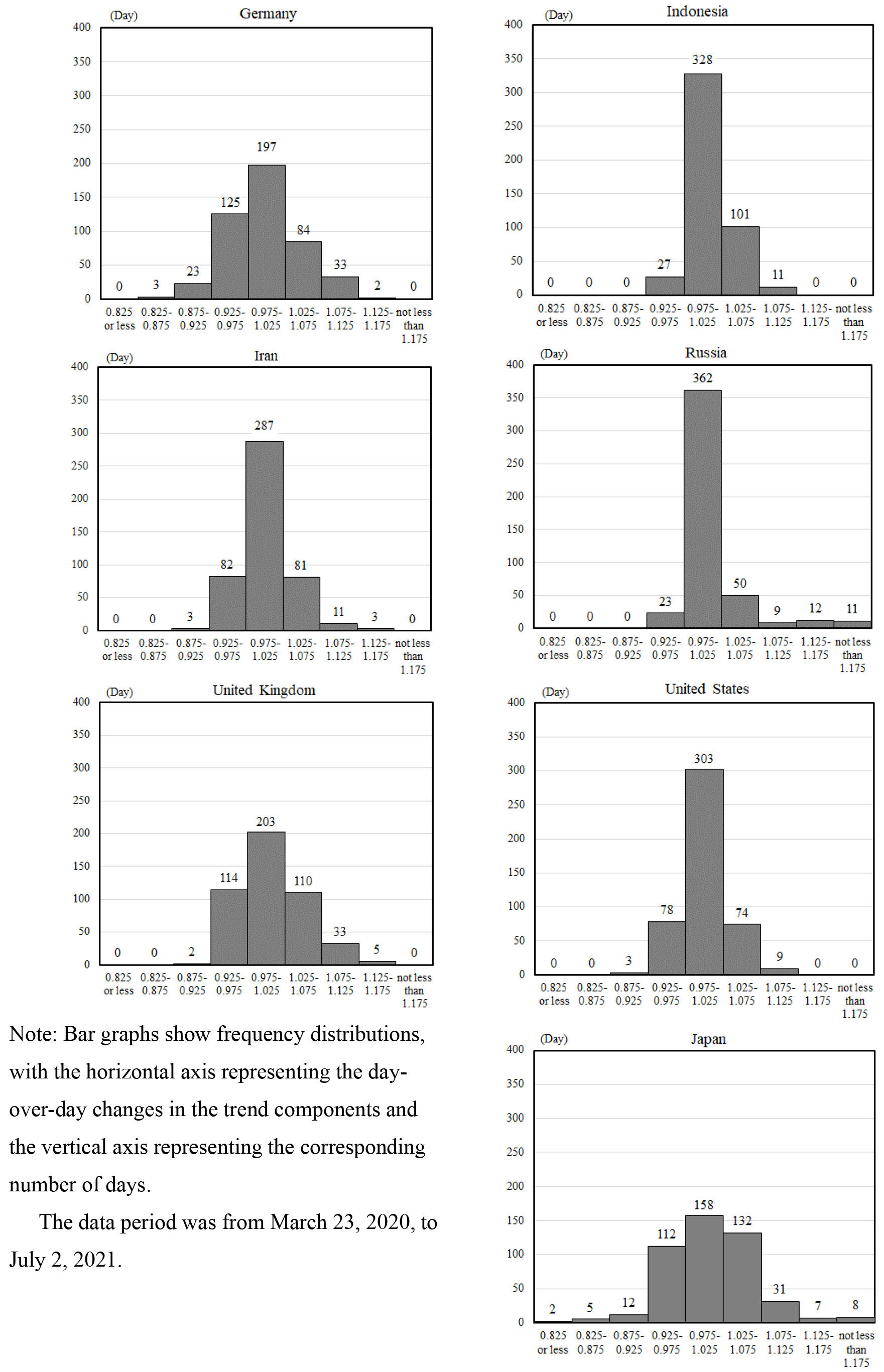
In addition, Fig. 8 illustrates the frequency distributions with the horizontal axis representing the day-over-day changes in the trend components and the vertical axis representing the corresponding number of days.
Figure 9.
Weekly periodicity components.
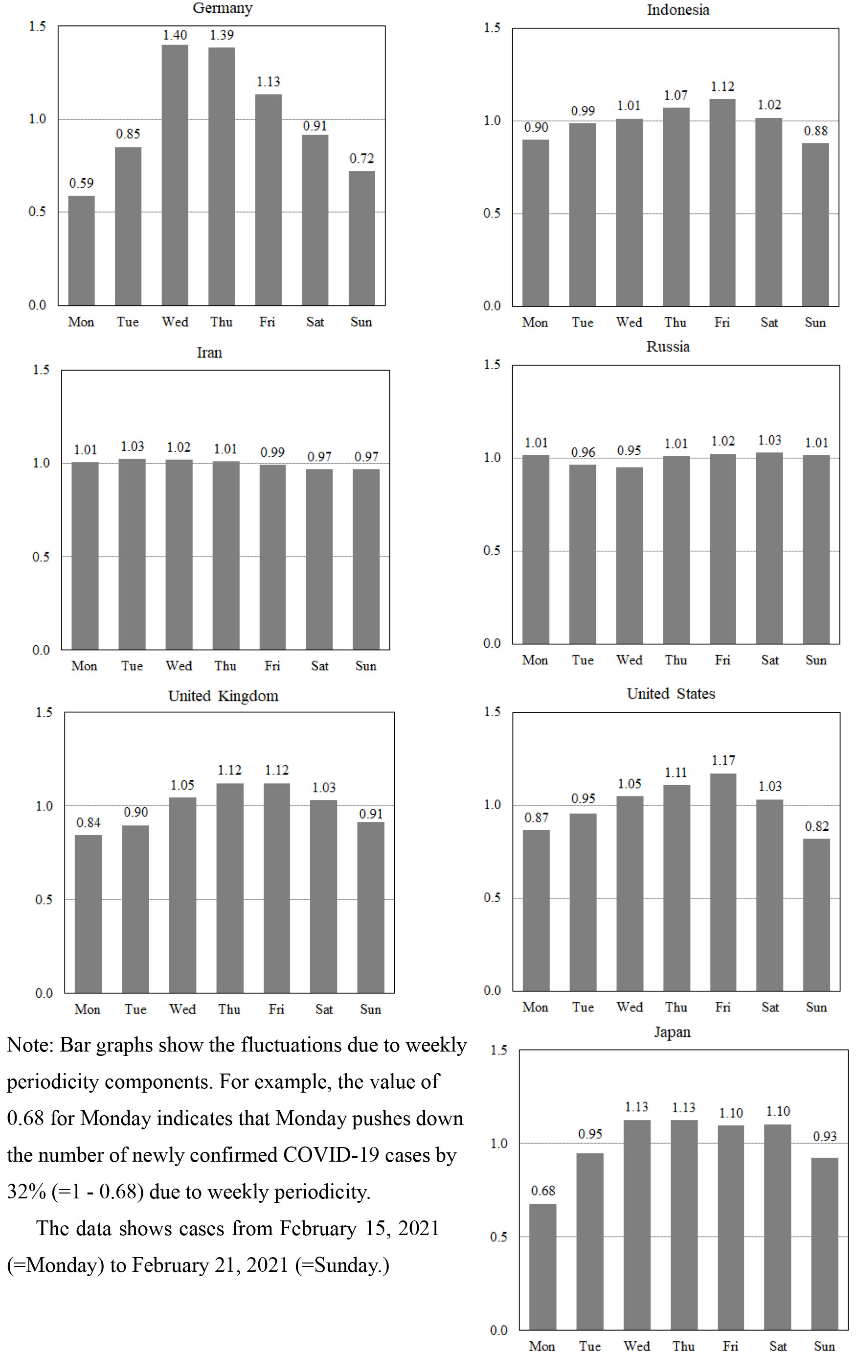
3.3Calendar-induced components (weekly periodicity and fluctuations due to moving holidays)
Figure 9 illustrates the estimated weekly periodicity in the number of newly confirmed COVID-19 cases. It indicates that weekly periodicity in Russia and Iran is small, but that in Germany is large. Besides, Table 3 reports the estimated downward effects due to moving holidays in the number of newly confirmed COVID-19 cases. As mentioned in 3.1 ‘Regression-ARIMA models,’ there are no significant fluctuations due to moving holidays in Russia and Iran.
Figure 10.
Spectrum of weekly periodicity components.
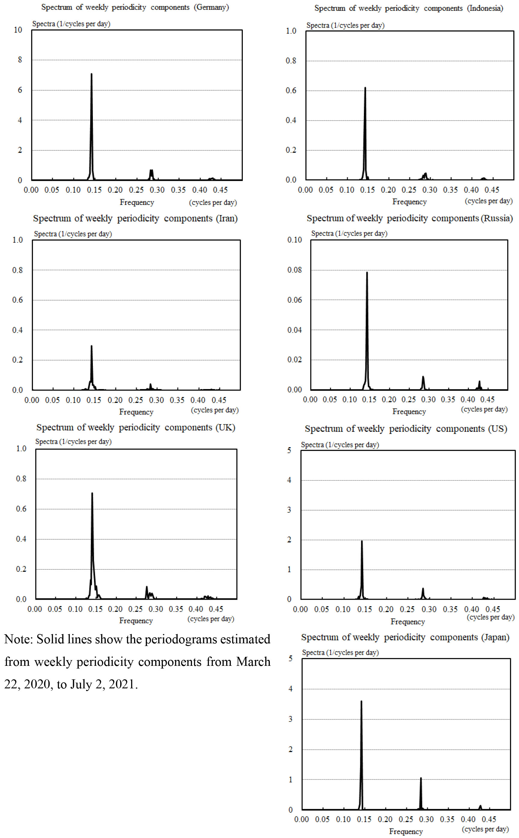
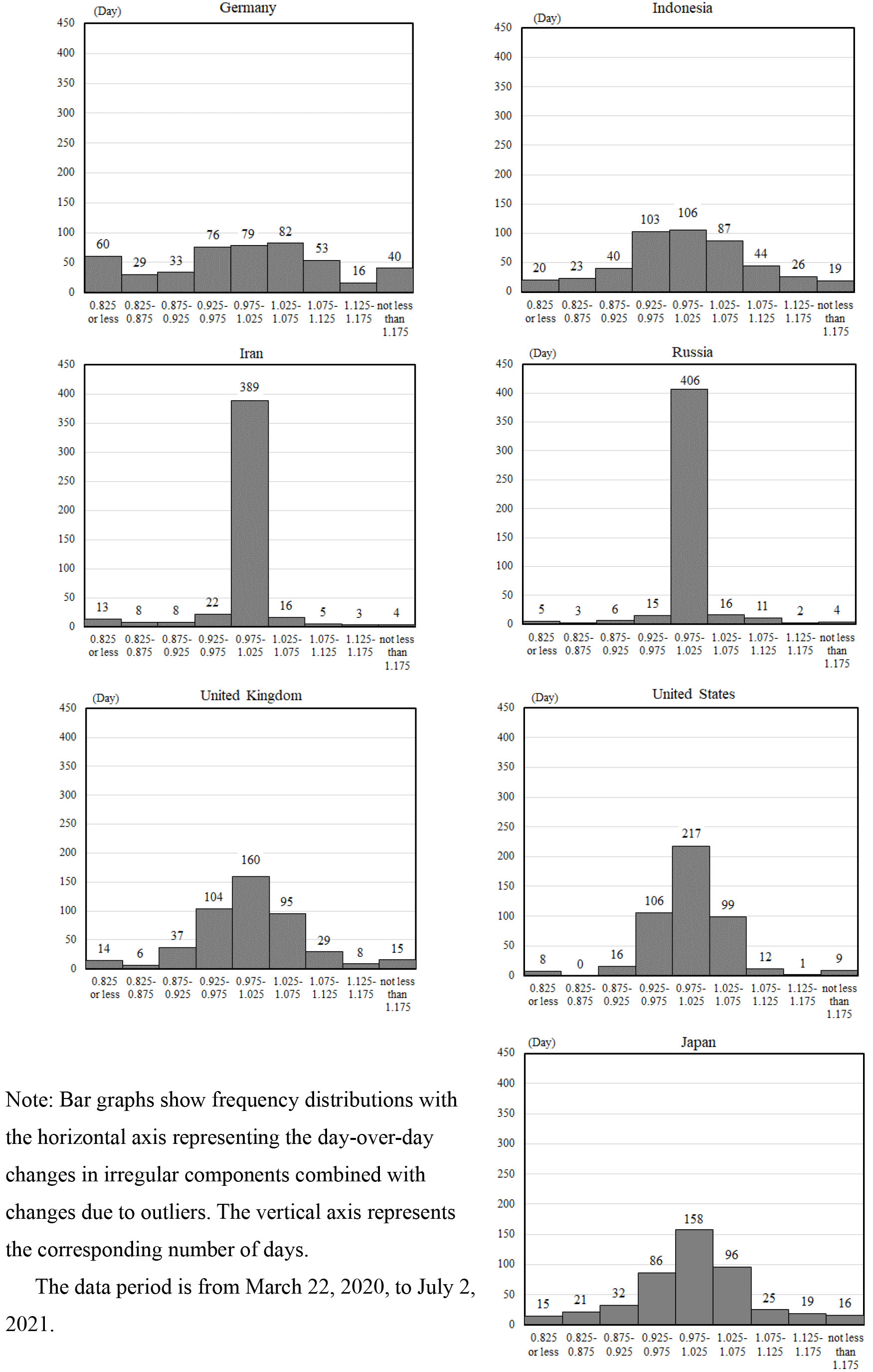
Figure 11.
Frequency distributions of irregular components.
In addition, Fig. 10 illustrates the periodograms estimated from the weekly periodicity components. The figure shows that the method in this study successfully extracts weekly-term changes from the original series.
Table 3
Downward effects due to moving holidays
| Downward effects due to moving holidays | Examples of moving holidays | |
|---|---|---|
| Germany | 0.777 | Neujahr (January 1, 2021) |
| Indonesia | 0.903 | Tahun Baru Imlek 2572 Kongzili (Febauray 12, 2021) |
| Iran | NA | – |
| Russia | NA | – |
| United Kingdom | 0.927 | New Year’s Day (January 1, 2021) |
| United States | 0.896 | Washington’s Birthday (February 15, 2021) |
| Japan | 0.740 | Emperor’s Birthday (February 23, 2021) |
Note: The value of downward effects shows the fluctuations due to moving holidays. For example, the Emperor’s Birthday in Japan indicates that the holiday pushes down the number of newly confirmed COVID-19 cases by 26.0% (
The downward effects of moving holidays appear without delay in Germany, the United Kingdom, and the United States. However, the downward effects of moving holidays appear to cause a delay by one day in Indonesia and Japan.
There were no countries where both 1-day lag and no lag regressors for moving holidays were significant.
Table 4
Estimated Markov-Switching models
| Regime 1 | Regime 2 | Turing point | |||
|---|---|---|---|---|---|
| Intercept | Standard error | Intercept | Standard error | ||
| Germany | 1.05 | 2.32 | 1.23 | 2020/9/4-5 | |
| Indonesia | 1.01 | 2.73 | 1.89 | 2020/11/4-5 | |
| Iran | 0.66 | 6.23 | 3.05 | 2021/3/26-27 | |
| Russia | 0.30 | 0.99 | 4.68 | 1.44 | 2021/6/8-9 |
| United Kingdom | 1.38 | 1.93 | 1.08 | 2020/4/15-16 | |
| United States | 1.92 | 2.29 | 1.67 | 2020/9/12-13 | |
| Japan | 0.92 | 0.32 | 0.79 | 2021/6/19-20 | |
| From | To | |
|---|---|---|
| Germany | 2020/8/26 | 2020/9/14 |
| Indonesia | 2020/10/29 | 2020/11/17 |
| Iran | 2021/3/10 | 2021/4/9 |
| Russia | 2021/5/19 | 2021/6/18 |
| UK | 2020/4/10 | 2020/4/19 |
| US | 2020/9/1 | 2020/9/20 |
| Japan | 2021/6/13 | 2021/6/29 |
Note: Markov-Switching Models are estimated by following time series of the percentage changes of the 7-day moving average:
3.4Irregular components
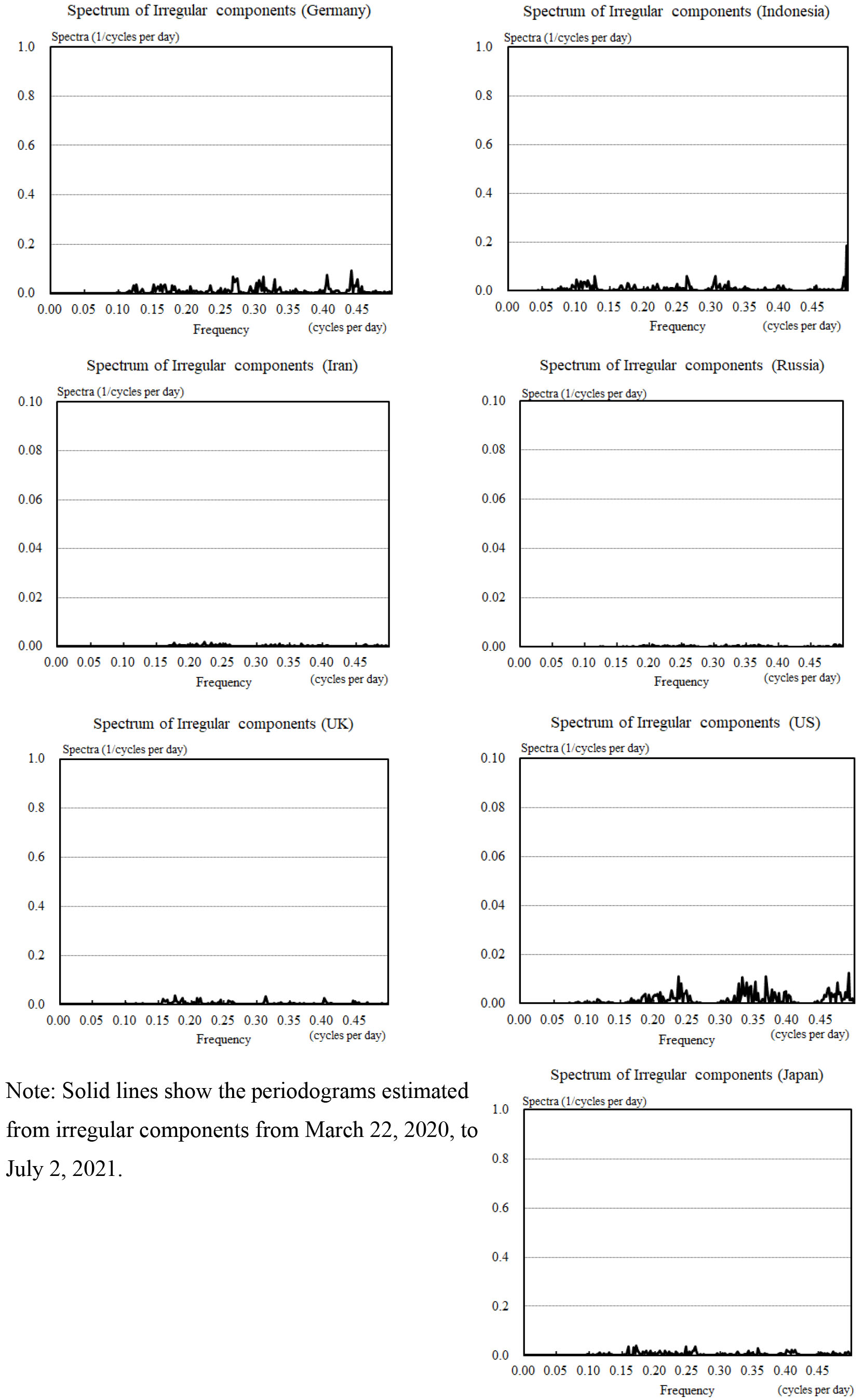
Figure 11 reports the frequency distributions of the irregular components in the number of newly confirmed COVID-19 cases. The distributions of all countries show symmetric distributions. Besides, Fig. 12 illustrates the periodograms estimated from the irregular components. There is no indication that trend components and weekly-term changes are mixed in with irregular components in Fig. 12. These two figures imply that the method in this study extracts the irregular variation correctly.
Figure 12.
Spectrum of irregular components.
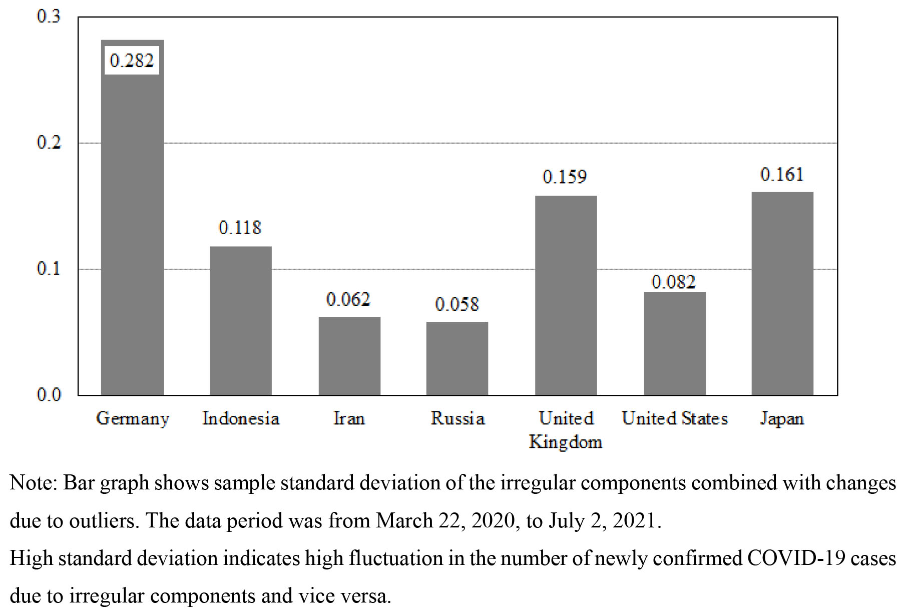
Additionally, Fig. 13 illustrates the standard deviation of the irregular components in the number of newly confirmed COVID-19 cases. It indicates that irregular fluctuations are high in Germany, followed by Japan and the United Kingdom.
Figure 13.
The standard deviation of irregular components.
3.5Evaluation of other periodicities
According to the periodograms (Figs 5, 7, 10, and 12), the evaluations of other low-frequency fluctuations including monthly periodicity, are as followings:
(i) Most changes in daily data are due to changes in trend components and weekly periodicity.
(ii) Other lower-frequency changes, including mon-thly periodicity, are significantly small in the daily data of this study.
3.6Pseudo real-time analysis
One aim of this study is the early identification of the trends in the number of newly confirmed COVID-19 cases. This sub-section shows the result of pseudo real-time analysis to check the timeliness of detecting the trends extracted by the method in this study compared with 7-day moving average. The steps of pseudo real-time analysis in this study are as follows:
(i) create time series of the change rates of the 7-day moving average in the vicinity of the turning point of the change rates. The periods of the time series are adjusted from 10 to 31 days depending on how fast the 7-day moving average changes.
(ii) estimate the turning points and change rates before and after the turning points by Markov-Switching Models using the time series of (i). Table 4 illustrates the details of the estimated Markov-Switching Models.
(iii) create multiple pseudo time series of the number of COVID-19 cases with different end dates. The end dates of pseudo time series are in the vicinity of the turning point.
(iv) estimate trends from the multiple pseudo time series by the method in this study and 7-day moving averages.
Figure 14 illustrates the change rates of estimated trends by this study and 7-day moving averages using multiple pseudo time series in the vicinity of the turning point. Regime 1 and Regime 2 show the change rates and standard errors before and after the turning point estimated by Markov-Switching Model.
Figure 14.
Pseudo real-time analysis of the trend and 7-day moving average.
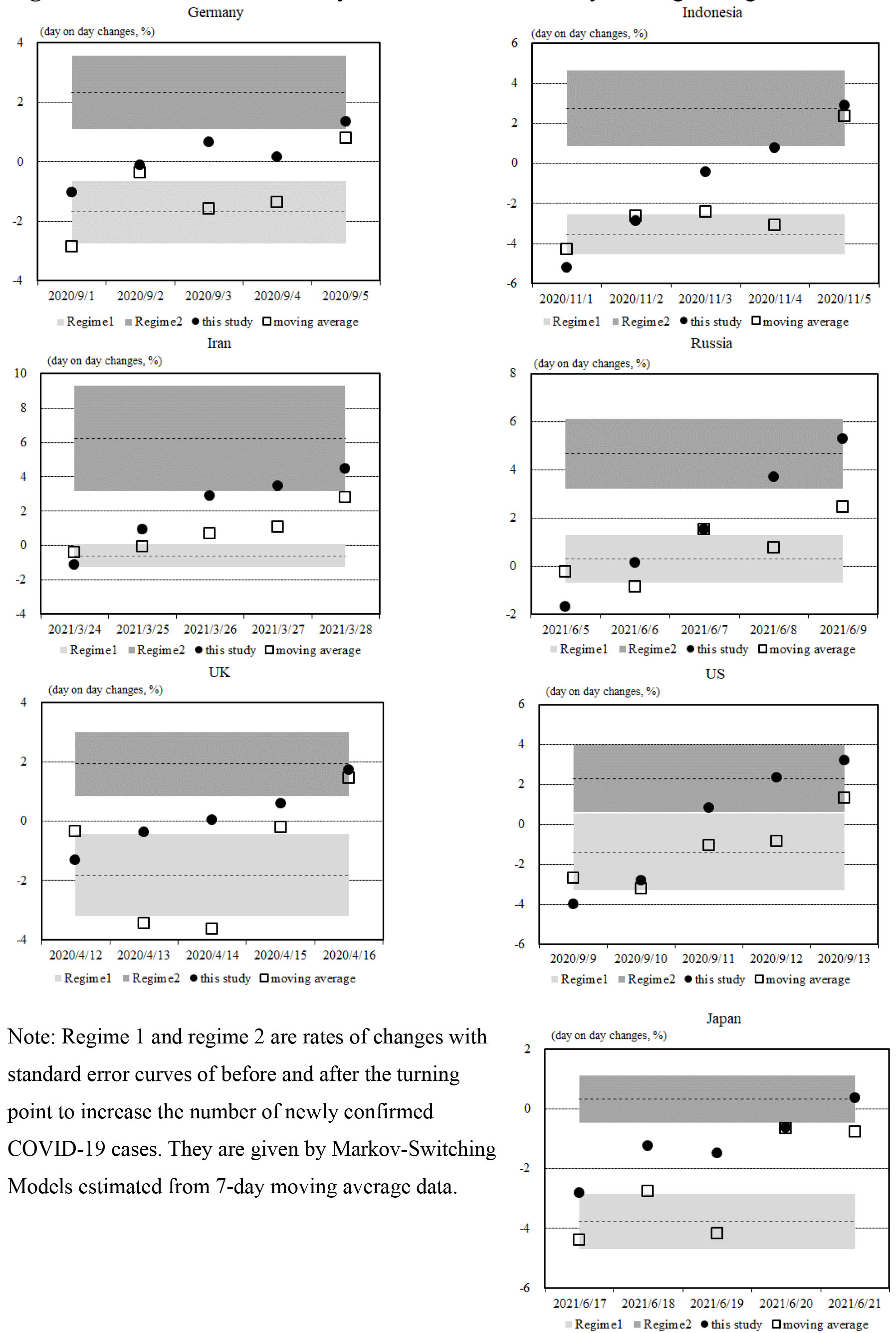
Firstly, the change rates of estimated trends by this study shift from Regime 1 to Regime 2 more smoothly than 7-day moving average. Secondly, in most cases, estimated trends by this study are ahead of 7-day moving average in the shift from Regime 1 to Regime 2.
Additionally, for generality, this study conducts the enhanced pseudo-real-time analysis for averaged trough (i.e., change from a “descending” regime to an “increasing” regime) and peak (i.e., change from an “increasing” regime to a “descending” regime). Moreover, to confirm the robustness of the method in this study, this study estimates models with the training subsets (i.e., data before the turning points). Due to the limitations to create the datasets, the enhanced pseudo-real-time analysis covers only UK and Japan.
Figure 15.
Enhanced pseudo-real-time analysis for averaged trough and peak periods.
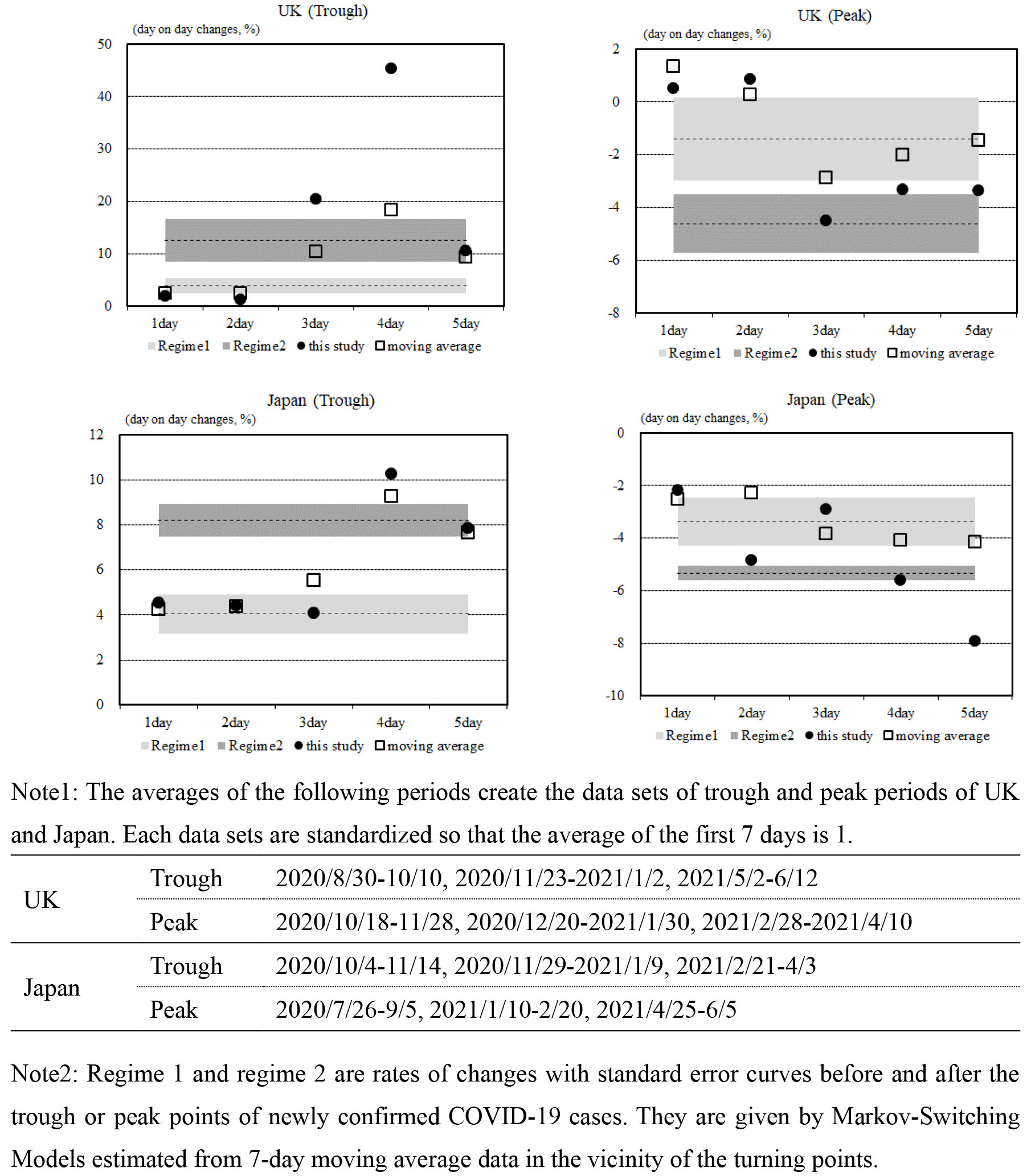
Figure 15 illustrates the change rates of estimated trends by this study and 7-day moving averages in the vicinity of the turning points. Excluding the trough period of Japan, estimated trends by this study are ahead of the 7-day moving average in the shift of regimes. This result supports the timeliness of detecting the estimated trends by this study.
Accordingly, analysis in this subsection illustrate that the method in this study is promising to identify trend changes of newly confirmed COVID-19 cases timely.
4.Discussion
4.1Main finding of this study
This study successfully extracts trend components, calendar-induced components, and irregular components from the data of newly confirmed COVID-19 cases of seven countries by X-13. At the same time, this study shows that the method can facilitate more rapid and accurate assessment compared to a 7-day moving average and a rolling 7-day total.
The characteristics of extracted components could be helpful to assess the risk of the spread of COVID-19 and develop strategic responses. Firstly, trend components are critical data to evaluate the spreading speed of COVID-19 and forecast the number of new cases. Additionally, calendar-induced components could indicate the characteristics of the observation system for COVID-19 cases, such as characteristics of the system for conducting PCR tests and reporting test results.
Furthermore, this study shows that the method can apply to other daily time series with weekly periodicity.
4.2What is already known on this topic
Previous studies on seasonal adjustment methods or the ARIMA model applied to the time series analysis of the number of newly confirmed COVID-19 cases have reported the following:
• Singh, Chowdhury, Panja, and Neogy [11] compared the predictions of the ARIMA model and the Holt exponential method to determine the number of newly confirmed COVID-19 cases in Sudan and found that the ARIMA model was preferable by the goodness-of-fit test.
• Liu et al. [12] applied the Ensemble Empirical Mode Decomposition (EEMD) method to the time series of COVID-19 confirmed cases in 10 countries to detect seasonal signals and quantify the impact of seasonality, e.g., temperature, on the spread of COVID-19.
• Fath et al., Abdelaziz, Alzahrani, and Shokeralla [13] analyzed time series models to test the lockdown effect in India. Additionally, the study applied the ARIMA-based forecasting model to predict the number of newly confirmed COVID-19 cases, COVID-19 tests conducted, and the average positive rate of the tests.
Previous studies on the application of seasonal adjustment methods to daily time series have reported the following:
• Ladiray, Palate, Mazzi, and Proietti [14] examined the application of ‘the X11 family,’ i.e., methods based on moving average like the X11, X11-ARIMA, X12- ARIMA, and X-13, to daily data and showed an actual example of electricity usage.
• Ollech [3] examined the procedure for adjusting changes due to various periodicity and moving holidays and showed an actual example of adjusting the fluctuations in German currency in circulation by STL.
Additionally, a previous study by the author applied X-13 with a modified X-11 methodology subprogram to the number of newly confirmed COVID-19 cases of Japan and Tokyo. It showed the feasibility of X-13 for identifying the trend in the number of newly confirmed COVID-19 cases [15].
4.3What this study adds
For the first time, this study shows that X-13 can apply to the analysis of changes in the number of newly confirmed COVID-19 cases, with implementations of seven countries.
The method in this study has the following advantages:
• Compared to a 7-day moving average and a rolling 7-day total, the method extracts more high-precision trend components due to eliminating the fluctuations of moving holidays and outliers.
• The method identifies trend changes timely thanks to Henderson moving averages, optimized to reproduce third-order polynomial.
• Calendar-induced components and irregular components extracted by the method are helpful to assess the risk of spreading COVID-19.
Moreover, this study shows that the method can apply to other daily time series with weekly periodicity by examples of the number of newly confirmed COVID-19 cases of seven countries.
4.4Limitation of this study
The method in this study successfully decomposes the number of newly confirmed COVID-19 cases into trend components, calendar-induced components, and irregular components. Nevertheless, there is no guarantee that the method works as expected for other daily data with weekly periodicity, especially the selection of the Henderson moving average and seasonal filters. Hence, it is necessary to accumulate practical implementations for verification of the method.
This study does not aim to identify annual patterns because the period of data to be analyzed is too short about one year and three months to extract annual patterns. However, improving this method to be able to identify annual patterns on an annual basis is a challenge for future analysis for long-time series.
Additionally, the target of the analysis in this study is limited to the number of newly confirmed COVID-19 cases. Hence, the method in this study cannot analyze the impact of factors that lead to changes in the number of newly confirmed COVID-19 cases (e.g., government response including requests for self-restraint and changes in weather conditions, such as temperature).
Acknowledgments
This study uses the dataset of Johns Hopkins University from ‘Our World in Data’ to obtain the number of newly confirmed COVID-19 cases. These data are compiled from patient information reports under challenging situations. Finally, the author wishes to express respect and gratitude to all the front-line medical institutions and health centers involved.
This study does not represent the official views of the Bank of Japan. All statements in this paper must be attributed to the author.
References
[1] | Tokyo Metropolitan Government. Updates on COVID-19 in Tokyo [Internet]. [cited 2021 Apr 10]. Available from: https://stopcovid19.metro.tokyo.lg.jp/en/. |
[2] | Public Health England. Coronavirus (COVID-19) in the UK [Internet]. 2021 [cited 2021 Apr 10]. Available from: https://coronavirus.data.gov.uk/easy_read. |
[3] | Ollech D. Seasonal adjustment of daily time series [Internet]. Deutsche Bundesbank Discussion Paper. 2018. Available from: https://www.bundesbank.de/resource/blob/763892/0d1c33f19a204e2233a6fccc6e802487/mL/2018-10-17-dkp-41-data.pdf. |
[4] | Findley DF, Monsell BC, Bell WR, Otto MC, Chen B-C. New Capabilities and Methods of the X-12-ARIMA Seasonal Adjustment Program. J Bus Econ Stat [Internet]. (1998) ; 16: (2): 127-52. Available from: doi: 10.1080/07350015.1998.10524743. |
[5] | Time Series Research Staff, Center for Statistical Research and Methodology, U.S. Census Bureau. X-13ARIMA-SEATS Reference Manual (Version 1.1) [Internet]. Washington, DC; 2017. Available from: http://www.census.gov/srd/www/x13as/. |
[6] | Bee Dagum E. The X11ARIMA/88 seasonal adjustment method - foundations and user’s manual [Internet]. Ottawa; 1999. (Statistics Canada technical report). Available from: https://www.census.gov/ts/papers/Emanual.pdf. |
[7] | Tiller R, Chow D, Scott S. Empirical Evaluation of X-11 and Model-based Seasonal Adjustment Methods. Methods. 2007; (December). |
[8] | Shiskin J, Young AH, Musgrave JC. The X-11 variant of the census method II seasonal adjustment program. 1967. (U.S. Census Bureau Technical Paper). |
[9] | Johns Hopkins University & Medicine. CORONAVIRUS RESOURCE CENTER [Internet]. 2021 [cited 2021 Apr 10]. Available from: https://coronavirus.jhu.edu/. |
[10] | Our World In Data. Coronavirus (COVID-19) Cases [Internet]. 2021 [cited 2021 Jul 4]. Available from: https://ourworldindata.org/covid-cases. |
[11] | Singh S, Chowdhury C, Panja AK, Neogy S. (Preprint in Research Square) Time Series Analysis of COVID-19 Data to Study the Effect of Lockdown and Unlock in India. 2020;7. Available from: https://www.researchsquare.com/article/rs-83179/v1. |
[12] | Liu X, Huang J, Li C, Zhao Y, Wang D, Huang Z, et al. The role of seasonality in the spread of COVID-19 pandemic. Environ Res [Internet]. (2021) ; 195: (April): 110874. Available from: doi: 10.1016/j.envres.2021.110874. |
[13] | Fath EE, Abdelaziz GMM, Alzahrani S, Shokeralla AAA. Prediction the daily number of confirmed cases of COVID-19 in Sudan with arima and holt winter exponential smoothing. Int J Dev Res [Internet]. (2020) ; 10: (September): 39408–13. Available from: https://www.journalijdr.com/prediction-daily-number-confirmed-cases-covid-19-sudan-arima-and-holt-winter-exponential-smoothing. |
[14] | Ladiray D, Palate J, Mazzi GL, Proietti T. Seasonal Adjustment of Daily Data. (2018) . |
[15] | Arita T. Applying the Seasonal Adjustment Method to the data of new confirmed COVID-19 cases in Japan(in the press, written in Japanese). J Heal Welf Stat, (2021) . |


