
The ILO nowcasting model: Using high-frequency data to track the impact of the COVID-19 pandemic on labour markets1
Abstract
The impact of the COVID-19 pandemic resulted in unprecedented labour market disruption, triggering the most severe global labour market crisis on record. The speed and depth of the crisis rendered labour force survey data unable to provide timely information. The ILO nowcasting model was designed to track the disruption in the world of work caused by the pandemic. This required: 1) filling data gaps, 2) increasing the timeliness of available data, and 3) focusing on an indicator that captured well the pandemic disruption: hours worked.
The estimates obtained from the ILO nowcasting model have become the backbone of the empirical strategy behind the ILO Monitor on the World of Work publication series. The latest estimates corroborate that the pandemic induced very large declines in hours worked at an unprecedented speed. Furthermore, the recovery process has stalled, driven by a stagnant recovery in developing economies. The country-level input data and estimates of the ILO nowcasting model allow for complementary analysis, which was published in the ILO Monitor. The topics included the effects of COVID-19 testing and tracing, fiscal stimulus, and vaccination on labour market outcomes.

1.Introduction
The COVID-19 pandemic has highlighted the importance of timely economic and labour market data. The containment measures taken to limit the spread of the virus and its devastating consequences caused a large decline in work activity, which materialized at unprecedented speed. Similarly, the lifting of restrictions was followed by strong – albeit incomplete – rebounds in hours worked. The labour statistics production system, primarily the collection and publication of labour force surveys, did not produce sufficiently timely and globally representative data. Even in countries with frequent data production exercises, such as quarterly labour force surveys, a delay of a few months after the quarter has elapsed can be expected. Moreover, in many countries, labour statistics are collected and published as annual data. These present large publication gaps, for instance, data for 2020 would only typically be published more than 12 months after the onset of the pandemic. In this context, nowcasting techniques, which leverage information from data sources that are timelier than the variable of interest, provide a good complement to the standard data production methods. This can be seen for instance in [1], an application to the United States labour market. Prior to the pandemic there was already strong interest in producing timely estimates via nowcasting, as in [2]. But demand for and relevance of timely estimates have increased substantially.
A suitable target variable needs to be chosen to track work activity during the pandemic at the global level. Standard indicators derived from labour force surveys, such as unemployment and employment, present limitations in the context of the economic shocks caused by the pandemic. For instance, because unemployment requires a person to be searching for a job, the common use of online job search tools can lead to a higher rate of unemployment based on this alone. Regulations of mobility during a lockdown could heavily influence the results for similar reasons. Unemployment requires one to be, besides searching for a job, available to work. This requirement would not be met if in-person work in non-essential activities was temporarily forbidden. As a result, unemployment might not increase during a lockdown due to its technical definition, even as the actual economic situation worsens. Moreover, economic policy responses to the pandemic also heavily affected employment measurement. Notably, job retention schemes proved to be very effective at stabilizing employment levels, even if workers could not carry out their usual activities. To track global work activity during the pandemic, a measure that comprehensively captures the nature of the economic shock caused by COVID-19 and with a high degree of international comparability is needed. Hours worked, as measured by labour force surveys, overcome these limitations of comparability, and provide a good overlap with concepts from the System of National Accounts.
To predict hours worked via nowcasting we use two different types of timely high-frequency indicators. The first type of indicator is available during the pre-pandemic period, prior to 2020Q1. These variables, which include amongst others retail sales, household and business confidence, and purchasing managers index (PMI), have been commonly used in economic nowcasting, including during the pandemic. The second type of indicator used only became available after the onset of the COVID-19 pandemic. The indicators in this category covered mobility data from mobile phone users, stringency of COVID-19 containment measures taken by governments, and COVID-19 epidemiological data. While these variables have no direct economic content, they provide a useful measure of the degree of disruption caused by the pandemic. For this reason, they are expected to contain information about the evolution of work activity.
From the methodological point of view, the current study divides the nowcasting problem into two types of estimation problems, according to the data availability situation of each country. The first would constitute a “classic” nowcasting problem. In these countries, a quarterly series of hours is available with some delay with respect to the target period. Moreover, countries in this category also have high-frequency indicators with a record prior to the pandemic. Hence, a projection for hours worked can be made based on the historical statistical relationship following a time-series/panel approach. In contrast, if high-frequency economic indicators are not available in a country, we exploit the cross-sectional variation of hours worked and high-frequency indicators related to the pandemic to project hours worked. These country-level estimates are aggregated at the global and regional aggregates.
From the perspective of the results, it is interesting to highlight that the latest estimates, published in the 9
2. Data
This section describes the data sources used in the ILO nowcasting model.
2.1Target variable
The first step in providing estimates tracking the labour market disruption caused by COVID-19 is finding a suitable indicator for this purpose. We focused the search for indicators on the most common source of labour statistics, labour force surveys. Labour force surveys are one of the primary national household surveys conducted by countries. They are designed to produce official national statistics on the labour force, employment and unemployment for monitoring and planning purposes. Labour force surveys are the main source behind headline indicators of the labour market for short-term monitoring as well as more structural information on the number and characteristics of the employed, their jobs and working conditions, the job search activities of those without work, etc. In the current study, the term labour force survey is understood to include household surveys that broadly follow standards set by the International Conference of Labour Statisticians (ICLS).
Within the substantial number of indicators that can be derived from labour force surveys, the commonly used indicators for assessing labour market trends related to economic activity such as unemployment and employment, present severe limitations in capturing the effects of the pandemic on the labour market. The limitations of unemployment as a labour underutilization indicator have been long established. Critically it is prone to undercount the actual degree of labour underutilisation. More comprehensive measures of labour underutilization, which capture those in time-related underemployment or those that are in the potential labour force22 were proposed in the 19
As the main purpose of the exercise is producing global and regional aggregates concerning work activity disruption, this and other differences between countries would greatly reduce the comparability of the data and hence complicate the econometric modelling of missing observations. Moreover, the objective of capturing disruptions in the world of work requires capturing declines in work activity caused by the pandemic and public health containment measures, even if they were offset or mitigated by public policy.
Hours actually worked, in contrast to employment or unemployment, are expected to capture the effect on work activity in a more comprehensive manner. Declines in hours can certainly result from job losses, but they can also derive from being employed and not at work (furlough schemes) or from a reduction in average weekly hours worked. Similarly, a fall in hours will capture diminished work activity of those who lost their job – regardless of whether they become unemployed or transition out of the labour force, see ILO Monitor [4]. The difference between a person who is unemployed and one outside of the labour force is defined by the answers to behavioural questions of a labour force survey. For instance, searching for a job is generally required to consider someone unemployed. In the context of the COVID-19 pandemic, the difference between the two might have become more ambiguous, as depending on public health measures job search would not have been possible, even if in other circumstances it would have occurred.
2.2 Hours worked: Data collection and treatment
The main source of hours worked data is ILOSTAT (https://www.ilo.org/ilostat/), the ILO’s repository of international labour statistics.44 There are several measures of hours worked captured in labour force surveys, we focus on hours actually worked. International standards, [5], define hours actually worked as the time persons spend in activities that contribute to the production of goods and services. Other measures, such as hours usually worked, would not be as useful in capturing short-term fluctuations in work activity. We include in our target variable only hours actually worked in the main job. Hours worked in secondary jobs tend to be much lower than hours spent in the main job (by an order of magnitude) and are not as widely available.
In the estimates used for the 9
Data availability is heavily skewed towards high-income countries. Table 1 summarizes the information. Whereas high-income countries only account for 30 per cent of the target countries, they account for 60 per cent of the actual observations. As national income decreases, so does the actual data coverage. At the lowest end of the spectrum, we find low-income countries, which account for 1 per cent of observations even if they represent 14 per cent of the countries. More recent data is also scarcer. The quarter with the most observations is 2020Q1, with 66 observations. In contrast, only 3 countries had some partial (monthly) data available in 2022Q1.
Table 1
Distribution of hours worked observations and distribution of countries and territories across income groups
| Income group | Distribution of actual observations (%) | Distribution of countries and territories (%) |
|---|---|---|
| Low income | 0.9 | 14.3 |
| Lower-middle-income | 9.4 | 28.6 |
| Upper-middle-income | 29.3 | 26.5 |
| High income | 60.4 | 30.7 |
To enhance comparability across countries and time, we divide hours worked by population. Given that countries present significantly different population growth rates, tracking activity without accounting for changes in the population would limit comparability. Countries with high fertility rates would tend to show higher growth rates of hours worked (or lower losses of hours worked) than countries with lower fertility rates. A similar argument can be made for the change in population in a given country over time. To properly capture work activity, changes in working hours need to account for this change to ensure that the level increase in population is not driving growth in hours worked (for the same reason, employment is often adjusted by population, using the employment-to-population ratio indicator). Population aged 15–64 is used in the normalization, as persons aged 15 to 64 tend to have much higher participation rates in the labour market than those 65 or older. Hence for each quarter, total hours worked are divided by population aged 15–64. The source of the population data is the United Nations World Population Prospects (UN WPP), 2019 edition. To avoid discontinuities population at the quarterly frequency based on the UN WPP annual data is estimated. These estimates simply assume a constant quarterly growth rate that is consistent with the annual one.
Given the objective of tracking the disruption caused by COVID-19 on work activity, we focus on relative changes with respect to a pre-crisis benchmark, which we define as 2019Q4. Hence the target of estimation for a country of interest is:
(1)
Where
(2)
In some instances, to simplify the text the “divided by population aged 15–64” is omitted, and population is used as a shorthand for population aged 15–64.
2.3High-frequency indicators
For nowcasting estimation, we require indicators that are available on a timelier basis than the target variable. In the present study, we use the shorthand high-frequency to refer to this circumstance.55 We can distinguish two different types of high-frequency indicators based on the temporal horizon of availability.
The first type of indicator is available during the pre-pandemic period, prior to 2020Q1. These variables, which include amongst others retail sales, household sentiment and business confidence, purchasing managers index (PMI), and labour market indicators have been commonly used in economic nowcasting, including during the pandemic, [7, 8]. The ILO compiled approximately 4’000 time series from various online repositories,66 roughly three-quarters of them available at the monthly frequency and the rest at the quarterly frequency. Table 2 presents the main types of indicators included in this repository. These indicators are highly unevenly distributed across countries. Around half of the target countries have only five or fewer high-frequency indicators, while 30 per cent of countries have more than 10 indicators.
Table 2
Main types of high-frequency indicators used in the model with a pre-pandemic record
| Type of indicator | Source |
|---|---|
| Business confidence | Trading Economics and country specific repositories |
| Capacity utilisation | |
| Car registrations | |
| Construction output | |
| Consumer confidence | |
| Foreign direct investment | |
| Industrial production | |
| International trade statistics | |
| Job vacancies | |
| PMI (Manufacturing, Services, Total) | |
| Retail sales | |
| Tourist arrivals | |
| Labour force survey data (employment, unemployment, etc.) | ILOSTAT |
| GDP projections | IMF, EIU |
The second type of indicator used only became available after the onset of the COVID-19 pandemic. The indicators in this category covered three broad areas: mobility data from mobile phone users, stringency of COVID-19 containment measures taken by governments, and COVID-19 epidemiological data. These three indicators are expected to contain information about the evolution of work activity. Larger declines in mobility, more strict containment measures and a worse epidemiological situation are expected to be associated with larger declines in work activity. All three indicators are available at a high frequency, either daily or weekly, and we average the data to the quarterly frequency.
The source of mobility data is the Google Community Mobility Reports. These reports contain aggregate changes in mobility compared to a pre-pandemic baseline. We take an average of the workplace mobility index and the retail and recreation index as input for the model.77 Other indices available in this dataset are related to behavioural changes during the pandemic and more indirectly related to economic activity and hence are expected to contain less information about the labour market and are not included in the model. As a proxy for stringency of COVID-19 containment measures taken by governments, we use the COVID-19 Government Response Stringency Index (hereafter “Oxford Stringency Index”). The source of the index is the Oxford Covid-19 Government Response Tracker (OxCGRT) database [9]. The index is a composite of restrictions across several dimensions, such as workplace closures and stay-at-home requirements. The indicator aims to capture quantitatively the degree of stringency of public health measures. As a proxy of a country’s COVID-19 epidemiological situation we use deceased patients per population. The source for the data is [10]. We expect this measure to be a more accurate reflection of the public health situation than COVID-19 cases, due to testing practices, the difference in vaccination rates and other potential comparability problems.
3. Methodology
This section describes in detail the methodology used in the ILO nowcasting model. We briefly outline here the main steps taken.
Our estimation target consists of 189 countries and territories, which are the basis of the aggregate estimates. These countries can be broadly split into two groups. The first group has an abundance of economic high-frequency indicators and a relatively timely time series of hours worked derived from labour force surveys. The second group generally lacks both economic high-frequency indicators and a recent time series of hours worked. Given these different data situations, two different approaches are taken.
The “direct nowcast” approach is taken for countries with an abundance of required data. Using an information set that is both more timely than the target variable and presents a time series overlap with the target variable a prediction can be produced – as is standard in nowcasting applications. Given the large number of potential explanatory variables (high frequency economic indicators), we choose a dimensionality reduction strategy. Particularly, we use Principal Component Analysis selecting the first three components (after detrending and adjusting for seasonality). In this manner, we obtain a suitable number of variables for inclusion in time series regressions, which are the basis of the “direct nowcast” model. These explanatory variables are then used in country-specific time series regressions or in panel data regression models. Even with the dimensionality reduction, a large number of specifications based on lags or country-specific vs. panel model structures are possible. A cross-validation approach is used for model selection. The models are selected and averaged based on their simulated out of sample error.
The “indirect nowcast” approach is taken for countries with insufficient high frequency economic indicators availability and a lack of timely hours data. For this purpose, we leverage high-frequency indicators concerning the impact of the pandemic in a given country, such as mobility indicators or stringency of public health measures taken. The ratio of hours worked in a given quarter relative to the pre-pandemic benchmark (2019Q4) is computed for selected countries from their labour force surveys. Additionally, from the “direct nowcast”, we have available timelier estimates, which are used as a proxy for actual hours worked. This change in hours worked (or change in estimates of hours worked) is extrapolated to countries without data based on the available high-frequency indicators measuring the impact of the pandemic. The extrapolation model follows a multiple linear regression model. The indirect nowcast approach allows producing an estimate for countries with minimal data sources.
The final step is aggregation. From the nowcasting models, we have available country level estimates (or data) of the ratio of hours worked, divided by population, in a given quarter compared to 2019Q4. The change in hours worked of each country must be weighted by the level of hours worked in each country in 2019Q4 to produce the global and regional aggregates. We estimate this figure based on a regression model using 2004–2019 data and population estimates. Once this variable is estimated the aggregation just requires adding up the contribution of each country.
In addition to the detailed description of each of these steps, the section ends by evaluating the performance of the model based on pseudo out-of-sample simulations.
3.1 Empirical strategy
Nowcasting hours worked at the global and regional level presents a substantial variation with respect to standard nowcasting applications. As described in [8], the nowcasting problem typically consists of predicting a variable of interest at time
In our set-up, the information set is similar to the description above. In contrast, we do not have any observation for the target variable. Knowing the evolution of global88 hours worked requires having complete time series available for every country up to time
We want to produce global aggregates of the evolution of relative hours worked considering population changes. For this purpose, we need to aggregate across the target countries indexed by
(3)
Notice that the population in the denominator does not correspond to the benchmark period 2019Q4, and rather it refers to the target period
The change in hours can also be reframed as a subtraction instead of a division:
(4)
Which in this case indicates the difference in the level of hours worked. This formulation is used to compute full-time job equivalents, which can be obtained by dividing by a pre-set workweek (such as a 48-hour workweek). This full-time job equivalent is widely used in the ILO Monitor publication series.
Given that we have complete population data, our estimation target requires either having observations or estimates of
The problem of estimating
The second type of estimation problem is applied to countries for which the quarterly time series of the target variable is not available. Moreover, the information sets of these countries do not have sufficient (or any) high-frequency indicators with a pre-pandemic record. Hence, the estimation target is the entire sequence since the pre-pandemic reference period, i.e.
3.2 Time-series and panel approach, “direct nowcast”
The direct nowcast approach exploits the historical relationship between the target variable, hours worked per population
The relationships can be estimated at the country level or within a panel structure. Models estimated at the country level allow the use of country-specific high-frequency data, and also the estimation of country-specific coefficients. Panel techniques require the use of common high-frequency data, i.e. the time series have to represent the same variable across countries. However, they also have a number of advantages. First, an estimate of the change in working hours can be made for countries with available high-frequency data, but without a historical time series of hours worked. Second, differences in the estimated change in hours worked are easily traced to differences in high-frequency data. Third, pooling many countries in a panel reduces the risk of overfitting the model. Our approach relies on both country-specific and panel regressions.
3.2.1Data preparation and cleaning
From the roughly 4’000 available time series, only around 1’000 are used. The reduction is due to two main discarding exercises. Some are discarded by the nature of indicator, for instance inflation time series are not used in the prediction model. A second filter is requiring that the data is timely enough, in the current edition of the ILO nowcasting model only time series available up to 2022 January (or 2022Q1) are used.
For the country-level approach, all high-frequency indicators can be used. For the panel approach, however, the high-frequency indicators display various overlapping and non-overlapping country coverages. A total of 50 different panels could be formed through the various combinations of high-frequency indicators as they are available across the various countries. Only a subset of the potential groupings is selected considering country coverage and the number of indicators in the decision set to identify a “best” panel grouping for each country. The decision rule selects for each country the grouping that maximises the product of the log of the number of countries in a grouping, the log of the number of indicators in a grouping, and the log of the minimum length of the time series in that grouping. This procedure yields a total of 11 different panels.
The dimensionality of the data is reduced using a principal component analysis. In preparation for that step, the series are first detrended where required,1010 and seasonally adjusted.1111 Up to the first three principal components are retained for the analysis. The principal components are created for all indicators available at a country level, and for the 11 identified panel groups of high frequency indicators.
3.2.2Modelling approach
While standard time series models can be used for countries with monthly data on hours worked, a mixed frequency approach is required for the countries with quarterly data. In [11] it is shown that using a mixed data sampling approach (MIDAS) leads to a more efficient estimation than the approach of aggregating the monthly frequency to the quarterly level. This should hold particularly for the COVID-19 crisis with its large, sudden changes. The standard MIDAS approach employs a distributed lag function to impose structure on the series with a higher frequency, thereby reducing the number of parameters to be estimated. In [12] it is shown that when mixing quarterly and monthly frequency data, it is beneficial leaving the parameters unrestricted, and hence estimating an unrestricted MIDAS (U-MIDAS).
The dependent variable
For the countries with monthly data, a simple linear model is specified as
(5)
The independent variables are represented by
For the countries with quarterly data, a U-MIDAS linear model is specified as
(6)
Where the independent variables are represented by
It is possible including a lagged dependent variable in the model, and if added this lag is statistically significant. However, our testing has shown that such a model specification produces a fairly muted response to changes in high frequency indicators. Since labour market dynamics in times of COVID-19 were uncharacteristically fast, we decided excluding a lagged dependent variable from the model.
The objective of this exercise is obtaining an estimate for the current full quarter, even though it might not be finished yet. For instance, high frequency data might be available for the months of April and May, but not yet for June. Nevertheless, an estimate for the full second quarter should be obtained, which in fact requires some forecasting in the sense that the month of June is to be projected without having any real-time data from it. When this is the case, the high frequency indicators are lagged by the appropriate number of periods to obtain a direct forecast. This forecasting is only used for those periods where no high frequency data are available.
3.2.3Model evaluation and averaging
The specified models can vary by the number of lags of the explanatory variables, but also by the composition of those. In particular, only one, two or three of the principal components were considered for inclusion in the analysis. Further variation stems from the fact that models can be estimated at the country level, but also as panel models. As described above, 11 different panels have been retained, which can all be estimated with the variation in composition and lags of the high frequency indicators. As a result, a large number of potential nowcasts could be produced for any of the countries.
The large number of countries and models requires using a procedure to derive the point estimates. To this aim, we mainly follow [13], who discuss a frequentist model averaging procedures in factor-augmented time series models. Model averaging outperforms individual model selection in face of model uncertainty, [14, 15]. Jackknife model averaging works well with our modelling framework [16]. In particular, the nowcasting procedure mixes non-nested models (including mixing panel and country level models), covers multiple countries, and it requires a relatively fast computation time. Jackknife model averaging identifies the weights in a linear combination of all errors of models so that their sum of squares is minimized. The errors are derived from leave-one-out cross-validation. In [16] it is shown that, in practice, it is better imposing non-negative weights, which results in corner solutions with many models receiving zero weights. An alternative approach is constructing weights based on the inverse of the root mean squared error (RMSE), which are also derived from leave-one-out cross validation.
Cross-validation provides a heteroskedasticity-robust model information criterion [17], and it mitigates the risk of overfitting. For time series applications of cross validation, in [18] it is shown that a block of
The prediction of the direct nowcast takes the following 5 steps:
1. Estimate the various models, at the country level and for the potential panels, varying the exogeneous variables and the lags selected. For each estimation, derive the leave-h-out cross-validation errors.
2. Identify the evaluation time period as the maximum time frame where all models have usable observations and hence cross-validation errors. All models need to be evaluated on the same observations, adjusting for lags and the available timeframe for different high frequency indicators.
3. Compute the optimal model weights, based on [16], for each country individually. Those weights can only be estimated for countries with a historical time series of hours worked.
4. Compute weights based on the inverse mean squared cross-validation error (MSCVE), which puts a positive weight on all models. The MSCVE covering all models is computed at the country level for those countries where possible, but also by evaluating the MSCVE at the global level. The two types of weights are then computed for each country considering only those models for which estimates exist. Countries without any historical data will only have the model weights based on the global average MSCVE.
5. Compute the change in hours worked by applying the weights to the model predictions. In total, 3 different model averages are computed: the Jackknife average, MSCVE-based spanning all models and evaluated at the country level, and MSCVE-based spanning all panel models and evaluated at the global level.
The last step involves selecting the final nowcast among the three model averages for those countries where applicable. While the Jackknife model average is the preferred selection, judgement can be applied at the individual country level. The increasing availability of real data with the progression of the pandemic enabled an automation of the judgement process by selecting the averaged nowcast that comes closest to the predicted value from a regression of hours worked relative to the fourth quarter of 2019 and the Oxford Stringency Index. Hence, stringency informs the judgement process, but the nowcast is only driven by country-specific high-frequency data.
3.3Cross-sectional approach, “indirect nowcast”
This section describes how estimates for those countries with more limited data availability are produced. This approach is based on the cross-sectional variation and is labelled “indirect nowcast”. From the direct nowcast, we have obtained a series of estimates of hours worked per population up to the target quarter. To simplify the notation, let estimates represent the actual observations whenever these are available. Hence, we can obtain the relative change with respect to 2019 produced via the direct nowcast:
(7)
Where the super script
The imputation of these countries aims to palliate bias in the sample of countries included in the direct nowcast, see [19, 20]. Indeed, if those were representative of the 189 target countries, we could simply produce global results from that subset of countries. Nevertheless, there are important differences between the countries with sufficient information to create a direct nowcast and those without, for instance in terms of national income. Even more relevant are the country differences in the evolution of the COVID-19 pandemic and the containment measures taken by governments. Quarterly hours worked respond strongly and rapidly to public health measures, hence pandemic evolution information can be exploited for estimation in missing data countries.
Given the wide availability of high frequency data on mobility (Google Mobility Reports data) and the Oxford Stringency Index, described above, we use those indicators as a proxy for the social and economic disruption caused by COVID-19. We expect (and do observe for countries with data) that larger declines in mobility and increases in stringency lead to larger declines in hours worked. Because each variable is expected to have substantial noise, in the baseline specification we combine both variables into a single index using Principal Component Analysis to capture the common variation. We refer to this index as
The relationship is heavily dependent on each quarter. For instance, during 2020Q2, the period when the strictest lockdowns occurred, the reaction of hours to the proxy of COVID-19 economic disruption was very strong. In contrast, by the end of 2020 a similar change in disruption was associated with much lower hour responses. This is to be expected, there are multiple structural factors that plausibly change the response of the economy to the disruption caused by the pandemic. For instance, governments and economic agents adapt their behaviour, cycles of contraction and recovery can have different elasticities of economic activity to changes in restrictions, public health measures taken evolve and so does the virus. Given this, we estimate the econometric model independently at each quarter.
Our preferred specification is the following simple linear regression model:
(8)
Where
Based on these approaches we can produce an estimate for all those target countries for which we do not have either reported observations or a direct nowcast estimate. Hence, we can produce an estimated value of the relative change of hours worked divided by population aged 15–64,
3.4Aggregation
Albeit we have an estimate for the relative change with respect to 2019Q4 of each quarter of interest based on the indirect nowcast, we cannot yet derive from it the change in hours worked at the global level,
The estimate of the benchmark of hours worked per population aged 15–64,
With an estimate for the benchmark of hours worked
(9)
It is worth highlighting that systematic errors in the country estimate of the benchmark of hours worked,
(10)
3.5Pseudo-out of sample evaluation
The practice of evaluating a model prediction based on pseudo out-of-sample error simulations is commonplace in econometrics. Whereas in many applications the focus is on comparing competing models, [21], the pseudo-out of sample error contains useful information to assess the uncertainty surrounding the prediction [22]. The empirical strategy of this type of evaluation reserves a certain subset of the data by the model. The predictions of the model for this subset are then assessed against the actual observations, by the use of a loss function. The label “pseudo” indicates that the econometrician has access to the information, even if the model does not use it.
Because the main objective of the ILO nowcasting model is producing global estimates of the evolution of hours worked,
Even if our focus of interest is global and regional aggregates, simulating the nowcasting error at the country level is highly informative – as country errors are the drivers of aggregate ones. We perform two exercises to analyse errors at the country level. One to evaluate the country-level direct nowcast error and another one to evaluate the indirect nowcast error. For the direct nowcast evaluation, we perform a one-step out-of-sample simulation exercise. Hence, for countries with a sufficient time series, we discard the last data point in the time series and predict its value following a rolling window approach. The direct nowcasting model is mostly used to do one step ahead predictions, hence we focus on this metric. We then compare this prediction with the actual data. To simulate the error at the country level for the indirect nowcast, we follow the same procedure as the one used for aggregate error simulation, described just above. Nonetheless, instead of aggregating the estimation from the 30 per cent of excluded countries and then computing the error – as in the aggregate error procedure – we now compute directly the root mean square error at the country level.
Table 3
Pseudo-out of sample performance indirect nowcast, aggregate results
| Time | Change in hours worked | RMSE |
|---|---|---|
| 2020Q1 | 1.4% | |
| 2020Q2 | 3.4% | |
| 2020Q3 | 2.2% | |
| 2020Q4 | 1.8% | |
| 2021Q1 | 2.2% | |
| 2021Q2 | 1.4% | |
| 2021Q3 | 3.2% |
Note: the simulations are based on a sample of 50 countries with sufficient data for analysis. Of those we use 70 per cent of the sample to estimate the model and 30 per cent of the sample to evaluate performance. The change in hours worked is based on the aggregate changes of the 30 per cent of the countries in the sample that have been excluded from the model input. The change is computed with respect to 2019Q4. The prediction error shows the difference between the predicted and the actual observation change in hours worked with respect to 2019Q4 for the aggregate computed using the excluded countries. Both the change in hours and the error are averaged across the different simulations.
Table 3 presents the results of the aggregate exercise. The results show that the model performs reasonably well, particularly during 2020. In 2020Q2 the average simulation result implied a decline in hours worked of 23.1 percent (with respect to 2019Q4), whereas the error estimate was 2.9 per cent. By 2021Q3, the performance deteriorates as the average simulation projects a decline in hours of 5.1 per cent with an error estimate of 3 per cent.
Table 4
Pseudo-out of sample performance direct nowcast, one-step ahead RMSE, country level results
| Mean | Median | 10 | 90 |
|---|---|---|---|
| 3.1% | 1.8% | 0.8% | 5.5% |
Note: The summary statistics are based on prediction errors for 57 countries. The prediction errors show the difference between the predicted and the realized observation of hours worked as a percentage of hours worked in 2019Q4.
Table 4 presents the results of the direct nowcast exercise at the country level. The model performance is reasonable – albeit errors suggest sizeable uncertainty. The average one-step ahead RMSE is 3.1 per cent, whereas the median RMSE is 1.8 per cent. The 10
Table 5
Pseudo-out of sample performance indirect nowcast, RMSE, country level results
| Time | Mean | Median | 10 | 90 |
|---|---|---|---|---|
| 2020Q1 | 1.4% | 1.0% | 0.2% | 3.1% |
| 2020Q2 | 3.0% | 2.2% | 0.8% | 6.0% |
| 2020Q3 | 2.0% | 1.7% | 0.4% | 3.7% |
| 2020Q4 | 2.0% | 1.9% | 0.4% | 3.3% |
| 2021Q1 | 2.2% | 1.8% | 0.6% | 4.0% |
| 2021Q2 | 1.8% | 1.8% | 0.6% | 3.4% |
| 2021Q3 | 2.1% | 1.6% | 0.6% | 3.9% |
Note: the simulations are based on a sample of 50 countries with sufficient data for analysis. Of those we use 70 per cent of countries to estimate the model and 30 per cent of countries to evaluate performance. The prediction error shows the difference between the predicted and the actual observation change in hours worked with respect to 2019Q4 for the excluded countries. The prediction of the change in hours worked is computed for the 30 per cent of the countries in the sample that have been excluded from the model input. The summary statistics of the errors are computed across the different simulations.
Table 5 presents the results of the indirect nowcast exercise at the country level. The average RMSE across countries and the country level median RMSE are generally not far from the aggregate error. Albeit the average and median RMSE tend to be lower than the aggregate error, this is not true in every period. The 10
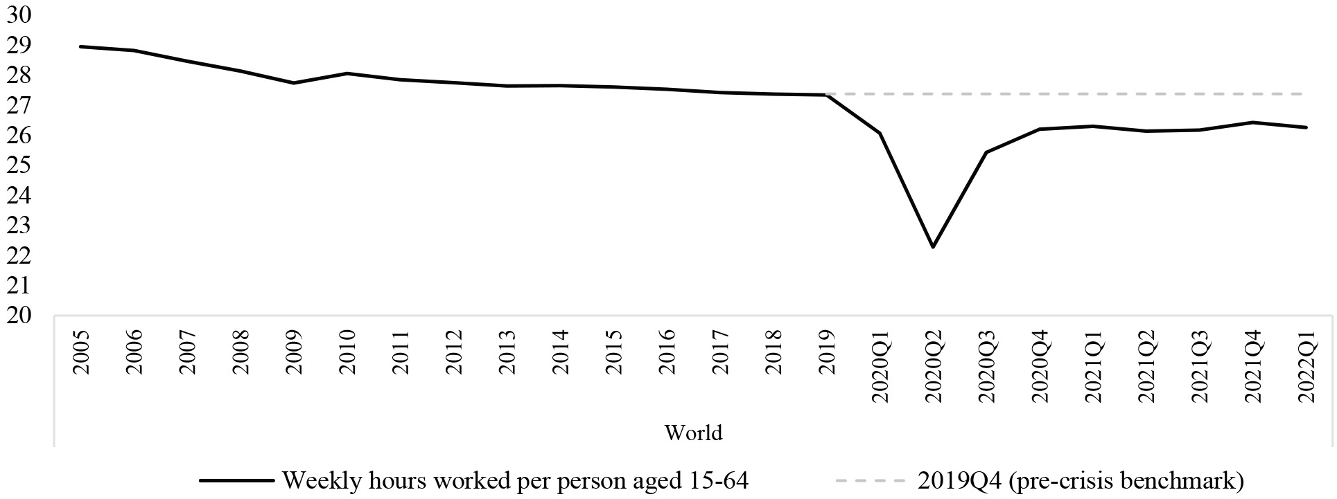
Figure 1.
Estimates of global weekly hours worked (divided by 15–64 population). Results of ILO Nowcasting model for the period 2005-2022Q1 at the global level. The 2005–2019 period is only estimated at the annual level, whereas from 2020Q1 and onwards quarterly estimates are available.
4. Results
4.1 A global view of the labour market during the pandemic
The latest estimates from the ILO nowcasting model, featured in the 9
As countries gradually lifted the strictest containment measures, hours worked recovered strongly. As a result, weekly hours increased to 25.4 in 2020Q3. By the end of the year, weekly hours worked per person aged 15–64 stood at 26.2, 1.2 hours below the pre-crisis benchmark. Both the initial decline and rebound were uncharacteristically fast, as labour markets tend to react with substantial delay in economic activity. In this instance the reaction was simultaneous1515 due to the nature of the economic shock. Nonetheless, the recovery in hours has been partial, and from 2020Q4 up to 2022Q1 hours have essentially stagnated. This left a gap of 1.1 weekly hours worked per person aged 15–64 remaining in 2022Q1. It is critical to highlight that given that hours are divided by population, it might well be the case that a recovery to the 2019Q4 level is never attained. Up to 2019, there was a slight but persistent declining trend in hours worked per person aged 15–64. If the trend persists into the future, the hours worked per capita would remain below the last quarter of 2019, even at very long-time horizons.
Figure 2.
Estimates of weekly hours worked (divided by 15–64 population) by income level, indexed data (2019Q4
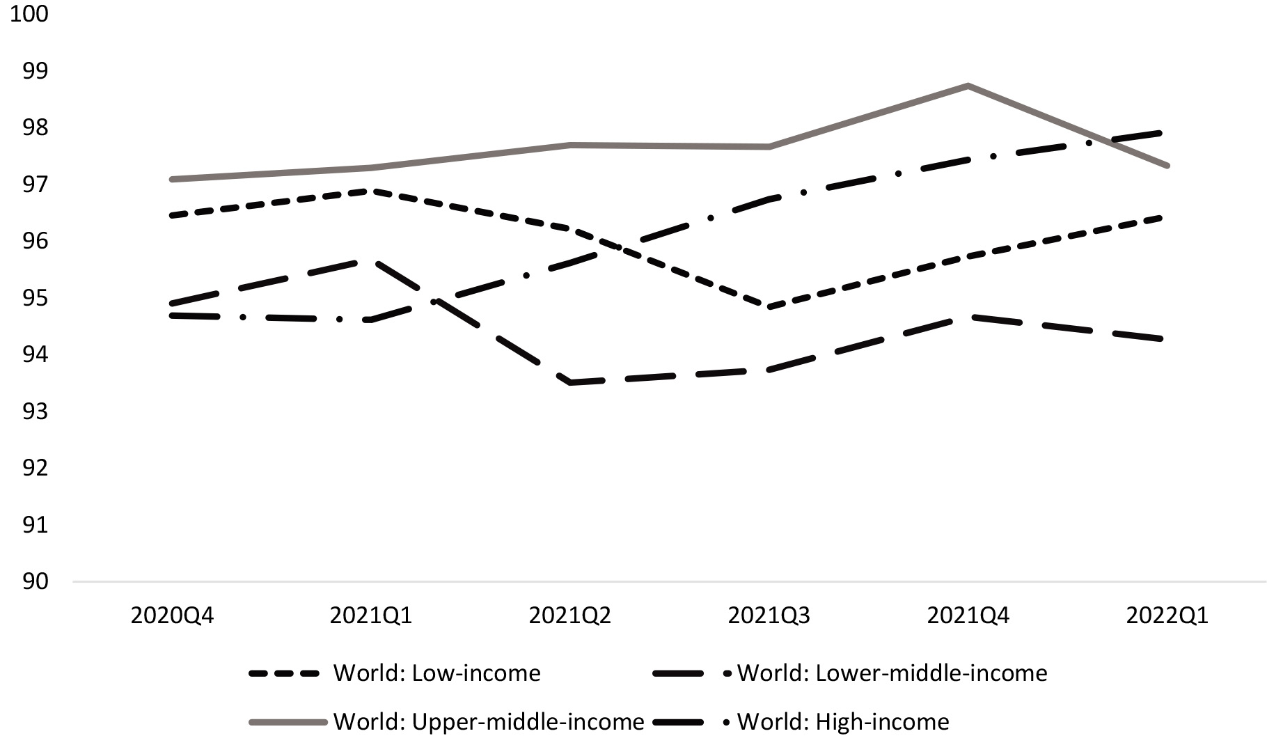
A key driver of the slow pace of recovery since 2020Q4 is the divergence between higher and lower-income countries (see Fig. 2). High-income countries experienced a strong recovery during 2021, becoming in 2022Q1 the income group with the levels of hours worked closest to the pre-crisis benchmark. Upper-middle income countries presented a sizeable recovery during 2021, which nonetheless was entirely offset by the lockdowns related to the Omicron variant of COVID-19 in China during early 2022. Low-income and lower-middle-income countries, in contrast, have presented a stagnant level of hours since 2020Q4. Uneven access to vaccination and lack of fiscal space to carry out stimulus programs at scale seems to have severely limited the recovery in low and lower-middle-income countries as shown in [23].
4.2 Timely analysis based on the ILO nowcasting model
Since its inception, the ILO Monitor on the World of Work has aimed producing timely and policy-relevant analysis. The work related to the ILO nowcasting provided two valuable sources of data (beyond the production of aggregate hours worked): an up-to-date, internationally comparable repository of hours worked, and timely country-level estimates. In this section, we highlight analysis in three key areas, based on these two data sources and published in the ILO Monitor publication series.
The first area of analysis was the effect of testing and tracing on labour market disruption, which was published in the early phase of the COVID-19 pandemic, [24]. At that stage, no actual observation for 2020Q2 was available, as the quarter had not yet elapsed, and labour force surveys present sizeable publication delays. The World Health Organization (WHO)1616 had recently re-iterated the importance of case finding, testing, contact tracing, isolation and care (which we shorten to testing and tracing). At that time, providing estimates of the potential economic effects of a policy recommended for public health reasons was useful to design policy measures for facilitating a safer return to work. Using the only data available for hours worked, estimates from the ILO nowcasting model, it was shown that following a strategy of intensive testing and tracing was associated with very substantial reductions in the loss of hours worked. The association suggested that moving from the lowest end of testing and tracing intensity to the highest end could reduce losses in working hours by 50 per cent.
The second area studied concerns the effects of fiscal stimulus on hours lost. In the 6
The third topic that we want to highlight is the effect of vaccination on the pace of recovery in hours worked. In the 8
5.Conclusion
The impact of the COVID-19 pandemic on the labour market has been unprecedented in both speed and level of disruption. Public health containment measures, and the lifting of those measures, have driven the dynamics of the global economy and labour market for the last two and a half years. In this context, data production by the standard labour statistical system (in particular, labour force surveys) was insufficient to meet the demand for timely and internationally representative data. Timely estimates produced by the ILO nowcasting model represented a solution to assess the impact of the pandemic on the labour market and track the subsequent recovery in a timely manner. The resulting estimates have become the backbone of the empirical strategy behind the ILO Monitor on the World of Work publication series. Moreover, the work related to the ILO nowcasting model produced as a “by-product” timely and internationally comparable country-level observations and estimates, which allowed for policy-relevant analysis during different phases of the pandemic.
Three main data types are used in the ILO nowcasting model. First, data from labour force surveys are used as the target variable to track work activity: hours worked. Second, high-frequency economic indicators with a relatively long time series (with observations available before the onset of the pandemic) are used as model input. These indicators include series as retail sales or industrial production and are often used in economic applications of nowcasting. Nonetheless, these indicators tend to be available only for a limited set of countries. Third, high-frequency indicators that only became available after the onset of the pandemic, such as mobility data from mobile phone users or stringency of COVID-19 containment measures, are used as input for the model in countries for which high-frequency economic indicators are not available or are likely to be non-representative.
Methodologically, two different models are set up according to the data availability. If a country has sufficient availability of high-frequency economic indicators, the historical statistical relationship between these and hours worked (based on that country or a panel of countries) is used to obtain more timely projections of hours worked. In contrast, if high-frequency economic indicators are unavailable in a country, we exploit the cross-sectional variation of hours worked and high-frequency indicators related to the pandemic to project hours worked. These country-level estimates are aggregated to compute global and regional aggregates. Simulations of out-sample results at the global level suggest that the model performance is satisfactory, albeit in later stages of the pandemic the predictive power seems to be deteriorating. Future work on the model needs focusing on the loss of statistical information of the key drivers of the indirect nowcasting procedure, which are related to pandemic circumstances and lack high-quality information concerning economic conditions. There are promising avenues, such as using other non-conventional data sources and increasing the number of low-frequency variables used in the extrapolation procedure.
The latest estimates, published in the 9
Notes
2 The potential labour force is conceptually close to unemployment but with less stringent requirements on search and availability.
3 The criteria used to define unemployment, such as searching for a job can see their usefulness reduced in a context of public health measures such as lockdowns.
4 This source is complemented with online information published by EUROSTAT and National Statistical Offices in certain cases to secure more timely and internationally comparable data.
5 This terminology is somewhat ambiguous since some of the indicators used in producing the estimates are actually collected at the quarterly frequency the same as the target variables (but are available on a timelier basis).
6 The main sources of data are ILOSTAT and Trading Economics.
7 In certain countries, the data presents an upward long-run trend, in which case the data is detrended.
8 An analogous procedure can be developed for regional aggregates; for simplicity, only the global aggregate is referred to in the text.
9 There are countries that constitute intermediate cases between the two categories which are assigned in an ad hoc manner to either group, for the sake of simplicity these are not mentioned in the discussion.
10 The series are only detrended if the procedure reduces the variation in mean and standard deviation over time.
11 Seasonal adjustment is made using Demetra
12 To allow for a log transformation, which we use in the econometric model, we ensure that the range of
13 For instance, let estimates of every single country be biased upwards by one per cent for both the benchmark and the relative change of hours worked. In the first case, the numerator and denominator will offset each other and hence the global difference induced by the bias will be zero. In contrast, in the second case
14 Systematic errors in the benchmark will have a larger impact on
15 Whereas there are no global estimates of quarterly GDP readily available, for countries for which data are available a similar trend for GDP can be observed. See https://data.oecd.org/gdp/quarterly-gdp.htm.
16 Dr Tedros Adhanom Ghebreyesus, WHO Director-General, opening remarks.
Acknowledgments
The authors thank Samuel Asfaha, Gillian Barmes, Janine Berg, Mario Berrios, Florence Bonnet, Marcela Cabezas, Juan Chacaltana, Marva Corley-Coulibaly, Rafael Diez de Medina, Sara Elder, Ekkehard Ernst, Luca Fedi, Mariangels Fortuny, Rosina Gammarano, Tite Habiyakare, Tariq Haq, Lawrence Jeff Johnson, Emmanuel Julien, Ken Chamuva Shawa, David Kucera, Sangheon Lee, Hannah Liepmann, Philippe Marcadent, Bernd Mueller, Martin Murphy, Mohammed Mwamadzingo, Federico Negro, Aurelio Parisotto, Yves Perardel, Mikhail Pouchkin, Gerhard Reinecke, Richard Samans, Dorothea Schmidt-Klau, Rosalia Vazquez-Alvarez, Sher Verick, Christian Viegelahn, Michael Watt, Johannes Weiss, Christiane Wiskow, Rosalind Yarde and Daniela Zampini for their helpful comments and suggestions. Additionally, the authors thank an anonymous reviewer whose comments and suggestions helped improve and clarify this manuscript.
The authors wish to acknowledge David Bescond, Vipasana Karkee, Quentin Mathys, Yves Perardel, Marie-Claire Sodergren and Mabelin Villarreal-Fuentes from the Data Production and Analysis Unit of the ILO Department of Statistics for their work on ILOSTAT. Finally, the authors wish to acknowledge the guidance and support during the entire project of Rafael Diez de Medina, director of the ILO Department of Statistics.
References
[1] | Coibion O, Gorodnichenko Y, Weber M. Labor Markets During the COVID-19 Crisis: A Preliminary View, NBER Working Papers 27017, National Bureau of Economic Research, Inc. (2020) . |
[2] | Evans M. Where Are We Now? Real-Time Estimates of the Macroeconomy. International Journal of Central Banking. (2005) ; 1: (issue 2). |
[3] | ILO. Resolution concerning statistics of work, employment and labour underutilization, in: 19th International Conference of Labour Statisticians, International Labour Organization. (2013) . |
[4] | ILO. ILO Monitor: COVID-19 and the world of work. Fifth edition, International Labour Organization. (2020) . |
[5] | ILO. Measurement of working time, in: 18th International Conference of Labour Statisticians, International Labour Organization. (2008) . |
[6] | ILO. ILO Monitor on the world of work. Ninth edition, International Labour Organization. (2022) . |
[7] | Jardet C, Meunier B. Nowcasting world GDP growth with high-frequency data. Journal of Forecasting. (2022) . 1–20. |
[8] | Bańbura M, Giannone D, Modugno M, Reichlin L. Now-casting and the real-time data flow. Working Paper Series 1564 July 2013. ECB. (2013) . |
[9] | Hale T, Angrist N, Goldszmidt R, Kira B, Petherick A, Phillips T, Webster S, Cameron-Blake E, Hallas L, Majumdar S, Tatlow H. A global panel database of pandemic policies (Oxford COVID-19 Government Response Tracker). Nature Human Behaviour. (2021) . |
[10] | Ritchie H, Mathieu E, Rodés-Guirao L, Appel C, Giattino C, Ortiz-Ospina E, Hasell J, Macdonald B, Beltekian D, Roser M. Coronavirus Pandemic (COVID-19). Published online at OurWorldInData.org. (2020) . |
[11] | Ghysels E, Santa-Clara P, Valkanov R. The MIDAS Touch: Mixed Data Sampling Regression Models. UCLA: Finance. (2004) . |
[12] | Foroni C, Marcellino M, Schumacher C. Unrestricted mixed data sampling (MIDAS): MIDAS regressions with unrestricted lag polynomials. Journal of the Royal Statistical Society: Series A (Statistics in Society). (2015) ; 178: (1), 57–82. |
[13] | Cheng X, Hansen BE. Forecasting with factor-augmented regression: A frequentist model averaging approach. Journal of Econometrics. (2015) ; 186: (2), 280–293. |
[14] | Steel J. Model averaging and its use in economics. Journal of Economic Literature. (2020) ; 58: (3), 644–719. |
[15] | Hansen BE. Least squares model averaging. Econometrica. (2007) ; 75: (4), 1175–89. |
[16] | Hansen BE, Racine JS. Jackknife model averaging. Journal of Econometrics. (2012) ; 167: (1), 38–46. |
[17] | Andrews DW. Cross-validation in regression with heteroskedastic errors. Journal of Econometrics. (1991) ; 47: , 359–377. |
[18] | Burman P, Chow E, Nolan D. A cross-validatory method for dependent data. Biometrika. (1994) ; 81: (2), 351–358. |
[19] | Crespi G. Imputation, estimation and prediction using the Key Indicators of the Labour Market (KILM) data set. Employment Strategy Paper 2004/16, (Geneva, ILO). (2004) . |
[20] | Horowitz JL, Manski CF. Censoring of outcomes and regressors due to survey nonresponse: Identification and estimation using weights and imputation. Journal of Econometrics. (1998) ; 84: , 37–58. |
[21] | Diebold FX, Mariano R. Comparing predictive accuracy. Journal of Business and Economic Statistics. (1995) ; 13: , 253–265. |
[22] | Stock J, Watson M. Phillips curve inflation forecasts, Conference Series; [Proceedings], Federal Reserve Bank of Boston, vol. 53. (2008) . |
[23] | ILO. ILO Monitor: COVID-19 and the world of work. Eighth edition, International Labour Organization. (2021) . |
[24] | ILO. ILO Monitor: COVID-19 and the world of work. Fourth edition, International Labour Organization. (2020) . |
[25] | ILO. ILO Monitor: COVID-19 and the world of work. Sixth edition, International Labour Organization. (2020) . |


