
Use of big data for official environment statistics: The measurement of extent and quality of freshwater ecosystems1
Abstract
The article describes how Big Data, such as geospatial and Earth Observation data, combined with advanced technologies, open opportunities for new ways of producing environment statistics. As an example of the use of Big Data, the article broadly presents SDG indicator 6.6.1 “Change in the extent of water-related ecosystems over time”, from the development of the methodology to the creation of datasets and their use by policy makers. The article also discusses the challenges of using geospatial and Earth Observation data both on a global scale and on a specific example of SDG indicator 6.6.1.

1.Introduction
Environment statistics is one of the main statistical domains along with economic and social statistics and covers a wide range of topics such as natural resources, soil, water, air, biodiversity, waste, climate change, natural disasters, environmental governance, material flow, environment and health.
According to the Open Data Inventory 2020/2021, provided by the international non-profit organization Open Data Watch, the average score for the coverage and openness of environmental data presented on the websites maintained by national statistical offices and any official government website that is accessible from the site of the national statistical office, at the global level is 46.9 per cent [1].
Since the adaptation of the 2030 Agenda for Sustainable Development, the lack of environment statistics has become more evident. As of July 2020, only 42 per cent of 92 SDG indicators relevant to the environment had sufficient data to assess progress made in achieving the SDG targets [2].
While environmental statistics are still at an early stage of development in many countries, Big Data, such as geospatial and Earth Observation data, coupled with advanced technologies, present opportunities for new ways of producing environment statistics [3].
2.Big Data as a source to produce environment statistics
The concept of Big Data gained momentum in the early 2000s when industry analyst Doug Laney articulated the now-mainstream definition of Big Data as the three V’s:
• Volume: Organizations collect data from a variety of sources, including transactions, smart devices, industrial equipment, videos, images, audio, social media and more;
• Velocity: With the growth in the Internet of Things, data stream into businesses at an unprecedented speed and must be handled in a timely manner;
• Variety: Data come in all types of formats – from structured, numeric data in traditional databases to unstructured text documents, emails, videos, audios, stock ticker data and financial transactions [4].
Big Data related to environment statistics are mainly based on geospatial and Earth Observation data.
Geospatial information provides the integrative platform for all digital data that have a location dimension. Geospatial data combine location information, attribute information, and often temporal information. Geospatial information is often derived from the Global Positioning System, which provides location and time information in all weather conditions anywhere on or near the Earth where there is an unobstructed line of sight to four or more GPS satellites.
Earth Observation (EO) is the gathering of information about planet Earth’s physical, chemical, and biological systems via remote sensing technologies (ground-based, airborne or spaceborne), usually involving satellites, unmanned aerial vehicles or other technology carrying imaging devices. Earth Observation is used to monitor and assess the status of and changes in the natural and manmade environment. As EO data are images of the Earth’s surface, they need to undergo corrective pre-processing of radiometric and geometric distortions before performing analysis, and are often integrated with administrative data, such as administrative boundaries or elevation during the analysis [5].
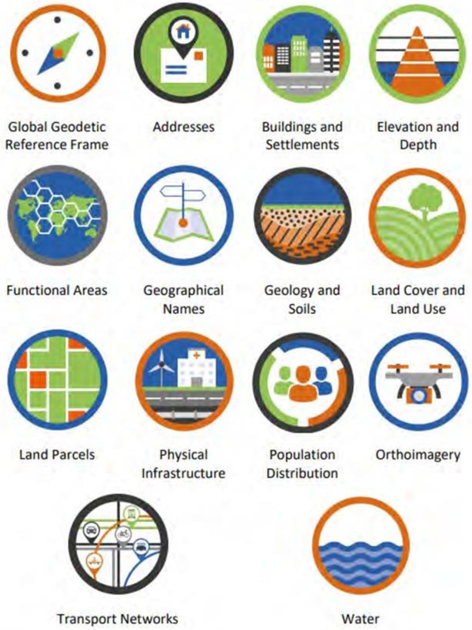
The United Nations Committee of Experts on Global Geospatial Information Management (UN-GGIM) has identified fourteen global fundamental geospatial data themes and geospatial data layers across environment, economic and social domains to support the SDGs, as illustrated in Fig. 1.
Figure 1.
Geospatial data themes.
A clear example of the demand for Big Data is the global set of indicators under the 2030 Agenda for Sustainable Development. Filtering an initial list of SDG indicators for which Big Data would be required, there are several environment-related SDG indicators which could be underpinned by geospatial and EO data [6]. These include indicators related to the following topics – land tenure and ownership, sustainable agriculture, water quality, water cooperation, water-related ecosystems, access to safe, sustainable, public transportation, land consumption, public land in cities, coastal eutrophication and marine litter, management of marine areas, marine and terrestrial protected areas, forest area, land degradation, mountain green cover, air, water and soil pollution and fishing. Additionally, geospatial data can be used for indicators related to the impact of climate change and disasters on populations.
2.1Challenges and considerations
At the same time, it is important to recognize that the integration of EO data into official statistics is confronted with a series of challenges.
Satellite imagery needs to be pre-processed to become analysis-ready for statistical purposes, and national statistical offices often lack technical skills for imagery pre-processing. However, access and availability of pre-processed imagery has been growing and technical capacity of practitioners is building through capacity development and other initiatives.
Other challenges include technical, human, and financial resources necessary for data storage, processing, and analysis. Despite the technological developments that render EO more accessible, these challenges need to be addressed to successfully integrate EO data into environment statistics.
In some countries, the Statistics Law limits the data sources that could be used to produce official statistics, hindering exploration of Big Data [7].
Close collaboration between national statistical offices, Mapping Agencies, Space Agencies and specialized Environment Agencies could help address many of those challenges. International development partners as well as the specialized funds and programmes of the United Nations that are custodians of the environment-related SDG indicators are supporting the national statistical systems in the use of EO data for environment and agriculture statistics through pilots, training and technical guidelines.
There are global groups which are leading the exploration of using Big Data for environmental monitoring and statistics:
• The United Nations Committee of Experts on Big Data and Data Science for Official Statistics (UN-CEBD) explores the application of EO data for official statistics;
• The Expert Group on the Integration of Statistical and Geospatial Information was established by the United Nations Statistical Commission (UNSC) and UN-GGIM. The Expert Group adopted the Global Statistical Geospatial Framework (GSGF), which enables the integration of geospatial and statistical information to facilitate data-driven decision-making.
• The Group on Earth Observation (GEO) is an intergovernmental partnership working to improve the availability, access and use of open Earth Observations. GEO’s priority engagement areas are the SDGs, Paris Agreement, and the Sendai Framework for Disaster Risk Reduction.
The scope of the use for Big Data extends beyond environment and environment-related indicators. Institutions are increasingly exploring non-traditional data sources to generate social and demographic indicators in cases where important data are missing. Combining administrative data with Big Data sources could provide timelier and more granular data and even generate new insights. The rapid advancement of modern technologies and their wide adoption by the public generate digital footprints, which, when repurposed in privacy-protecting and ethical ways, could provide valuable insights on populations and their pattern of movement [8]. Furthermore, crises often require real-time data, particularly on the location, density and movements of a population, while preserving personal data privacy and protection.
Population data can be integrated with environment statistics to estimate how environmental phenomenon affect the population. Data related to the geographical impact of a hazard can be integrated with census data to determine how a population is affected by disaster. Climate change analysis represents another area where Big Data can be integrated with census data to determine how human activities correlate with climatic phenomena. Conversely, climate change analysis can show the correlation between climate related disasters and mobility patterns, such as forced migration, internal migration and urbanization and expansion of artificial surfaces. Collecting socioeconomic data in a geographic context and maintaining the original location information could reveal patterns in the data, which would otherwise be missed.
3.SDG indicator 6.6.1 “Change in the extent of water-related ecosystems over time”, as an example of environmental indicators based on Big Data
Freshwater, in sufficient quantity and quality, is essential for all aspects of life and plays a fundamental role towards the achievement of many Targets and Goals within the 2030 Agenda for Sustainable Development. Freshwater ecosystems, which include lakes, rivers, reservoirs, wetlands, mangroves and groundwater – supply water and food to billions of people, provide unique habitats for many plants and animals and protect us from droughts and floods. While freshwater ecosystems hold less than 1 per cent of all water on Earth and cover just 0.8 per cent of the Earth’s surface [9], these ecosystems harbour exceptional diversity, hosting 10 per cent of all plant and animal species, including more fish species than have been found in the world’s oceans [10].
Globally observable changes to freshwater ecosystems and hydrological regimes are caused by human activities and climate change. Demand for water from the increasing population has redefined the natural landscape into agriculture and urban land. Freshwater quantity and quality are compromised as human activities demand more water for agriculture, power generation, urbanisation, industry, mining, flood management and domestic water supply. Global warming and associated changes in precipitation and temperature patterns will lead to more extreme weather events and exacerbate current anthropogenic stresses on the freshwater ecosystems. Today freshwater ecosystem changes are readily apparent in most countries observed through flow alteration; loss of connectivity; pollution; habitat degradation and loss; and overexploitation of species [11].
In recognising the extensive role freshwater ecosystems play within the development domain and to ensure planetary health, obtaining robust statistical trends of the extent to which freshwater ecosystems are changing can positively inform social, economic and environmental policy agendas.
SDG indicator 6.6.1 tracks changes in different types of water-related ecosystems – lakes and rivers; reservoirs; seasonal water bodies; coastal mangroves and inland wetlands such as peatlands and marshes; and groundwater. It is the only indicator used to measure national progress towards SDG target 6.6 which seeks to protect and restore water-related ecosystems. The indicator data are intended to inform policy relating to the sustainable and equitable utilisation of freshwater resources so that sector-based decisions consider their impact upon both the quantity and quality of freshwater within ecosystems.
3.1Freshwater ecosystems monitored using Earth Observations: General overview
In developing the methodology for indicator 6.6.1, UNEP set up a technical expert group that included representatives from the International Water Management Institute, the Convention on Biological Diversity, Ramsar (the Convention on Wetlands), the European Space Agency, and GEO.
This group provided inputs into the development of the monitoring methodology. A first draft methodology was piloted in 2017 and sent to all UN Member States accompanied with relevant capacity support materials. A limited number of Member States (19 per cent) submitted national in-situ data on freshwater ecosystem changes to UNEP after a period of 8 months. The data received were of poor quality and with limited spatial and/or temporal coverage. For those countries who did not submit any data the main reasons cited were a lack of data to report, and neither time nor resources to initiate new ecosystem monitoring.
Following on from the global piloting and testing phase, and to address a known global data gap for the indicator, the methodology was revised to incorporate data on water-related ecosystems derived from satellite-based Earth Observations. UNEP engaged with a series of partners working with global satellite missions and data products considered relevant and suitable for the indicator. The assessment of global data sources considered data quality, resolution, frequency of measurements, global coverage, time series, scalability and ability to provide disaggregated data at national and sub-national levels. The result was a methodology that is statistically robust producing internationally comparable data without being too onerous for countries to report on. The technical expert group was consulted on the updated methodology before submission to the Inter-agency and Expert Group on SDG Indicators (IAEG-SDG) for approval.
In 2018, the IAEG-SDG approved the indicator methodology and agreed that the indicator is conceptually clear, has an internationally established methodology and standards are available, and data are regularly produced for at least 50 per cent of countries and of the population in every region where the indicator is relevant.
The Working Group on Geo-Spatial Information of the IAEG-SDG reported that global datasets can serve as a sound basis for supporting the preparation of global reports. International agencies may use high quality global datasets to calculate SDG indicators and send disaggregated national level data to national authorities for review and agreement. To support countries in fulfilling monitoring and reporting requirements for SDG indicator 6.6.1, UNEP has worked with partner organisations, such as the Joint Research Centre (JRC) of the European Commission, Google, the US National Aeronautics and Space Administration (NASA), the European Space Agency (ESA), the Japan Aerospace Exploration Agency (JAXA), Global Mangrove Watch, DHI A/S, the UNEP-DHI Centre on Water and Environment (UNEP-DHI), Aberystwyth University, Brookman Consult, and Plymouth Marine Laboratory, to develop technically robust and internationally comparable global data series based on the approved methodology and thereby significantly contributing towards filling the global data gap on measuring changes in the extent of water-related ecosystems.
Data on permanent water, seasonal water, reservoirs, wetlands, mangroves, as well as lake water quality are available for countries to freely access at the SDG 6.6.1 indicator data portal [12]. Data are visualised for users on geo-spatial maps with accompanying numerical statistics displayed through informational graphics.
Table 1
Satellite data sources currently used for status reporting on SDG indicator 6.6.1
| Ecosystem type | Satellite data source | Website |
|---|---|---|
| Permanent, seasonal, reservoir | NASA Landsat (1984-present) | United States Geological Survey |
| (USGS) Earth Explorer | ||
| (https://earthexplorer.usgs.gov/) | ||
| Inland vegetated wetlands | European Sentinel-1 (2014-present); European Sentinel-2 (2016-present) | Copernicus.eu (https://www.copernicus.eu/en) |
| Mangroves | Japanese L-N | Jaxa.jp (https://global.jaxa.jp/) |
| Water quality | European Sentinel-3 (2017-present); European Envisat Medium Resolution Imaging Spectrometer (MERIS) (2002–2012) | Copernicus.eu (https://www.copernicus.eu/en) |
SDG indicator 6.6.1 intends to track longer term trends in ecosystem extent changes (i.e. over several years) rather than short term fluctuations. The SDG 6.6.1 data portal therefore provides statistical information for each water-related ecosystem type showing the extent to which it is changing over time. Water-related ecosystems (lakes, rivers, wetlands) may span large areas, be numerous in numbers and highly dynamic by nature. These characteristics make water-related ecosystems hard to access in their entirety. Numerous in-situ data collection points may be required to accurately measure changes to water quantity, quality and spatial area, over time. In this context there is substantial benefit to utilising satellite data sources to measure water-related ecosystems. Satellite images are numerical data, which can be processed into information and in turn transformed and aggregated into meaningful indicators for administrative areas such as national and river basin boundaries.
Globally satellite data are publicly available in high spatial resolution (10–30 meters) and with high temporal revisit time (days to weeks). To statistically represent a change in the extent of an ecosystem type between two periods of time, it is necessary to first define the reference period (or baseline) against which ‘change’ is then measured.
Not all data series represented on the SDG 6.6.1 site use the same reference period. This is due to the availability of recorded observations captured by different satellites. Some satellites, such as the American (NASA) Landsat satellites, have been orbiting Earth since the early 1970’s. These satellites have enabled the measurement of changes in the spatial area of open water bodies (i.e. lakes) since this time although early images were of lower quality thus reducing confidence in the outputs. More recently, additional satellites have been placed in Earth’s orbit, for example the Sentinel missions of the European Copernicus programme and several Japanese satellite missions, allowing image and data capture for other types of water-related ecosystems and parameters (e.g. wetlands, water quality and mangroves). Depending on when the satellites first started capturing data, this results in different reference periods for the various water-related ecosystem types within SDG indicator 6.6.1 (Table 1).
To encourage both national and sub-national decision making towards protecting and restoring water-related ecosystems, data are made available at national and sub-national levels. To depict national statistics the approved UN base map is used, while HydroBASINS is used to provide statistics for watershed boundaries at basin and sub-basin scales for the whole world [13]. An additional advantage of compiling 6.6.1 data using watersheds or river catchments is that it makes it possible to address issues at the regional and trans-boundary levels. It is important to note that for global reporting purposes, it is the national statistics per ecosystem type that are reported. The purpose of presenting watershed statistics within the SDG 6.6.1 data portal is to facilitate the process of sub-national and transboundary decision making on water-related ecosystems. Decisions relating to a particular water body (e.g. a lake) may often be taken by sub-national authorities, and in transboundary contexts coordinated decisions between multiple countries are required.
3.2Global mapping and calculation of changes in lakes and rivers
Data on the spatial and temporal dynamics of naturally occurring surface water have been generated for the entire globe [14]. The dataset captures long term changes (since 1984) in surface waters with a 30
![Expert system for global surface water mapping [14].](https://content.iospress.com:443/media/sji/2022/38-3/sji-38-3-sji220041/sji-38-sji220041-g002.jpg)
The data discriminate between permanent and seasonal waters. A permanent water surface is underwater throughout the year, while a seasonal water surface is underwater for less than 12 months of the year. Seasonal waters include temporarily inundated areas such as wetlands and paddy fields as well as lakes and rivers which freezes for part of the year. Areas of permanent ice, such as glaciers and ice caps as well as permanently snow-covered land areas are not included. Dams and reservoirs are removed using a different expert system designed to separate natural and artificial water bodies. Finally, a global shoreline mask [15] has been applied to prevent ocean water being included in the surface water statistics.
The dataset also serves to document various water transitions based on monthly observations of water presence or absence. Such water transitions include new permanent water surfaces (i.e. conversion of a no water place into a permanent water place.); lost permanent water surfaces (i.e. conversion of a permanent water place into a no water place) as well as new and lost seasonal water. The monthly time series can be used to identify specific months/years in which conditions changed, e.g. the date of filing of a new dam, or the month/year in which a lake disappeared.
The accuracy of the global surface water map was determined using over 40,000 control points from around the world and across the 36 years. The validation results show that the water detection expert system produced less than 1 per cent of false water detections, and that less than 5 per cent of water surfaces were missed [14]. However, it should be noted that it has been estimated that approximately 10 per cent of the world’s inland waters are within mixed pixels at the Landsat resolution, indicating a need to increase spatial resolution to track surface water changes more accurately [16].
The dataset has been integrated into the SDG 6.6.1 portal and every year new annual data are produced and added to the time series and used to update the statistics on changes in permanent and seasonal surface waters.
Changes in permanent and seasonal surface waters are calculated against a fixed baseline. The SDG indicator 6.6.1 methodology uses a 5-year baseline period (2000–2004). The baseline can be compared against a target period defined as any subsequent 5-year period. For each 5-year period the water state (permanent, seasonal or no water) is decided by a majority rule, and the water transitions between the baseline and the target period is subsequently used to compute the percentage change in the spatial extent of permanent and seasonal waters.
Changes in permanent and seasonal surface waters are calculated using Eq. (1):
(1)
The subject to the following for computing permanent surface water dynamics:
While the following applies for computing seasonal water dynamics:
The nature of this formula yields percentage change values as either positive or negative, which helps to indicate how spatial area is changing. On the SDG 6.6.1 data portal, statistics are displayed using both positive and negative symbols. For interpretation of the statistics, if the value is shown as positive, the statistics represent an area gain while if the value is shown as negative, it represents a loss in surface area. The use of ‘positive’ and ‘negative’ terminology does not imply a positive or negative state of the water-related ecosystem being monitored. Gain or loss in surface water areas can be beneficial or detrimental. The resulting impact of a gain or loss in surface area must be locally contextualised. The percentage change statistic produced represents how the total area of lakes, rivers within a given boundary (e.g. nationally) is changing over time.
Percentage change statistics aggregated at a national scale should be interpreted with some degree of caution because these statistics reflect the areas of all the lakes and rivers within a country boundary. For this reason, sub-national statistics are also made available including at basin and sub-basin scales. The statistics produced at these smaller scales reflect changes to a smaller number of lakes and rivers which are hydrologically connected within a basin or sub-section of a basin, allowing for localised, water body specific, decision making to occur.
Known limitations of the data are:
• Narrow rivers and lakes smaller than 30 meters by 30 meters are not captured as are those water bodies obscured by floating, overhanging and standing vegetation or hidden by infrastructure such as tunnels and bridges;
• Irrigated fields that stand in open water for some weeks are mapped but not when crop cover is well established;
• Temporal and spatial gaps can occur due to the combined effect of the Landsat revisit time (16–18 days), cloud cover and insufficient sunlight in higher latitudes.
3.3Global mapping and calculation of changes in reservoirs
The SDG 6.6.1 portal also includes a dataset that documents the long term (since 1984 onward) extent dynamics of 8,869 reservoirs. The reservoirs dataset represents the surface area of artificial water bodies including reservoirs formed by dams, flooded areas such as opencast mines and quarries, and water bodies created by hydro-engineering projects such as waterway and harbour construction.
The reservoir’s dataset is derived from the surface water dataset, which is fed into an expert system classifier designed to separate natural and artificial water bodies. The expert systems classifier is non-parametric to account for uncertainty in data, incorporate image interpretation expertise into the classification process, and uses multiple data sources. The expert system has been developed to delineate natural and artificial water using an evidential reasoning approach; the geographic location and the temporal behaviour of each pixel; and fed with datasets representing surface water extent, a priori knowledge and land surface topography. Table 2 lists the variables used to map reservoirs and dams globally. The dataset will be progressively complemented and continuously updated to account for newly built reservoirs.
Table 2
List of variables used to map reservoirs and dams globally
| Dataset | Description |
|---|---|
| Global Surface Water Explorer | This dataset that maps the location and long term (since 1984 onward) temporal distribution of surface waters surfaces at global scale at a 30 m spatial resolution. The maps include natural (rivers, lakes, coastal margins and wetlands) and artificial water bodies (reservoirs formed by dams, flooded areas such as opencast mines and quarries, flood irrigation areas such as paddy fields, and water bodies created by hydro-engineering projects such as waterway and harbour construction). Source: Pekel et al., 2016 https://global-surface-water.appspot.com/ |
| Global Reservoir and Dam Database | The Global Reservoir and Dam Database v1.3 is the output of an international effort to collate existing dam and reservoir datasets with the aim of providing a single, geographically explicit and reliable database for the scientific community. The initial version (v1.1) of GRanD contains 6,862 records of reservoirs. The latest version (v1.3) augments v1.1 with an additional 458 reservoirs and associated dams to bring the total number of records to 7320.Source: Lehner et al., 2011https://globaldamwatch.org/grand/ |
| ALOS World 3D | A global digital surface model (DSM) dataset with a horizontal resolution of approximately 30 meters (1 arcsec mesh). The dataset is based on the DSM dataset (5-meter mesh version) of the World 3D Topographic Data.Source: https://www.eorc.jaxa.jp/ALOS/en/aw3d30/aw3d30v11_format_e.pdf |
| The Shuttle Radar Topography Mission (SRTM) | A digital elevation dataset at 30 meters resolution provided by NASA JPL at a resolution of 1 arc-second.Source: Farr et al., 2004 |
The changes in reservoir area is calculated both as a change in minimum reservoir extent and as change in maximum reservoir extent. The calculation of minimum water extent is like the calculation of permanent surface water dynamics (Eq. (1)) but performed only for water bodies identified as reservoirs. The calculation of maximum reservoir extent also relies on Eq. (1) but using an extended set of parameters presented on Eq. (2):
(2)
where:
The percent changes in reservoir extent comes out as either positive or negative values, which shows where reservoir areas are changing. As a managed ecosystem, reservoir surface water extent might be expected to have less variability than natural surface waters. However, many countries and river basins show signs of either increases or decreases in reservoir extent – a pattern that can be explained by two main trends. First, within the past five years there have been many droughts in Brazil, India and South Africa, causing many reservoirs to reach critically low levels. Second, in the past decades there has been a global boom in new reservoirs, mainly along some of the world’s largest river systems, in particular the Yangtze, Euphrates, Tigris and La Plata rivers. Still, and like the permanent and seasonal water statistics, the observed gain or loss in reservoir areas must be locally contextualised to fully understand their nature, causes and impacts.
Known limitations of the data are:
• Some reservoirs built prior to 1984 may be missing;
• Reservoirs smaller than 3 hectares (30 000 square meters) may be missing;
• Branches of reservoirs whose width is smaller than 30 meters may be missing.
3.4Global mapping and calculation of changes in wetlands
In the context of SDG indicator 6.6.1 a high-resolution global geo-spatial mapping of inland vegetated wetlands has been produced detailing the spatial extent of wetlands per country. The data on inland wetlands have been produced to support countries with monitoring their wetland ecosystems and bridge an existing global data gap. The mapping included the entire land surface except for Antarctica and a few small islands. Only inland vegetated wetlands were mapped according to the following definition: “Vegetated wetlands include areas of marshes, peatlands, swamps, bogs and fens, the vegetated parts of floodplains as well as rice paddies and flood recession agriculture”.
Figure 3.
Workflow for mapping global wetland extent.
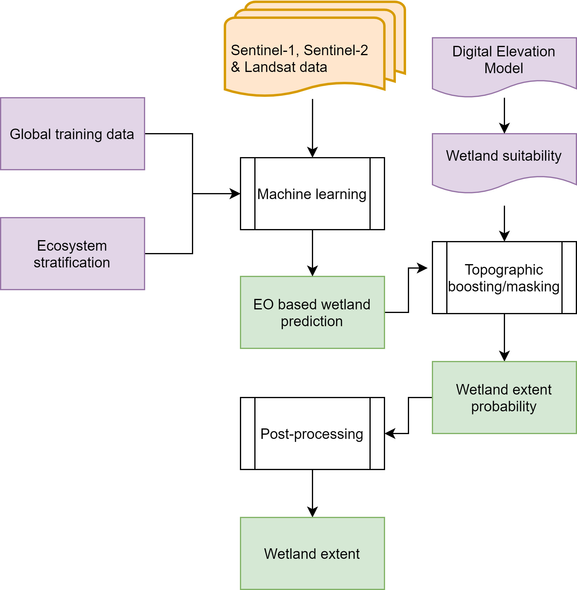
As wetlands tend to be susceptible to high annual variations, multi-annual data were collected to create a consistent wetland mapping approach based on satellite EO data. Predicting wetland extent using EO data relies on four components: stratification, training data, machine learning, and post-processing, as shown in Fig. 3. The approach uses all available data from 2016 to 2018 acquired by the satellites Sentinel-1, Sentinel-2, and Landsat 8 to predict wetland probability. Close to 4 million satellite images amounting to 2.8 petabyte of data were analysed and classified as wetland or non-wetland using an automated machine learning model and a representative set of training samples from the world’s major ecoregions. A Digital Elevation Model is used to qualify wetland predictions and a post-processing routine converts the wetland probability map into a map of wetland extent. Wetland area baseline statistics (in square kilometers) were calculated for all nations. Future annual updates will enable wetlands change statistics to be produced and once available these will be displayed on the SDG 6.6.1 data portal.
Data accuracy for the available wetlands data is approximately 70 per cent [17] and users should be aware that the map represents a first line rapid assessment of the global distribution of vegetated wetlands. While it is based on the best practical approach, there will inevitably be inaccuracies in the wetland predictions both in terms of commission and omission errors. Notable commission errors are for instance high-intensive irrigated agriculture parcels being classified as wetlands because they resemble many of the inherent spectral characteristics of wetlands (i.e. high moisture and vegetation presence even in dry season). Omission errors will mainly be attributed to the large diversity of wetlands. Despite best efforts to train the model across the widest range of wetlands possible, there will be types of wetlands and instances of wetland behaviour that will not be adequately captured in a global model. For instance, some ephemeral wetlands are rarely flooded or wet and therefore often missed by satellite datasets. In other cases, the wet part of a wetland may occur under a dense vegetation canopy, which is difficult to assess using EO data, where the presence of water/moist conditions is not easily detected. It is also worth noting that since the map only considers vegetated wetlands it may generate underestimations compared to national statistics which typically integrate metrics on surface water and coastal/marine wetlands.
Other known limitations of the data are:
• Only regional stratification is applied. Using a finer level stratification and additional training data will help improve local/national wetland predictions;
• Terrain information from satellite derived DEMs is key input for mapping wetlands globally. The current reference datasets are the 30-meter SRTM DEM which covers the globe from 60 degrees North to 56 degrees South [18], while the region north of 60 degrees North relied on a lower resolution 90-meter DEM model [19]. Options for 30-meter DEMs north of 60 degrees North exists and should be considered in future updates [20];
• Small islands and potentially even entire small island states fall outside the acquisition plan of the Sentinel satellites. As a result, no wetland prediction has been performed for these areas.
3.5Global mapping and calculation of mangrove area
Global mangrove area maps were derived in two phases, initially producing a global map showing mangrove extent (for 2010) and thereafter producing six additional annual data layers (for 1996, 2007, 2008, 2009, 2015 and 2016). The method uses a combination of radar (ALOS PALSAR) and optical (Landsat-5, -7) satellite data. Approximately 15,000 Landsat scenes and 1,500 ALOS PALSAR (1
The maps for the other six epochs were derived by detection and classification of mangrove losses (defined as a decrease in radar backscatter intensity) and mangrove gains (defined as a backscatter increase) between the 2010 ALOS PALSAR data on one hand, and JERS-1 SAR (1996), ALOS PALSAR (2007, 2008 & 2009) and ALOS-2 PALSAR-2 (2015 & 2016) data on the other. The change pixels for each annual dataset were then added or removed from the 2010 baseline raster mask (buffered to allow detection of mangrove gains also immediately outside of the mask) to produce the yearly extent maps.
Classification accuracy of the 2010 baseline dataset was assessed with approximately 53,800 randomly sampled points across 20 randomly selected regions. The overall accuracy was estimated to 95.3 per cent, while User’s (commission error) and Producer’s (omission error) accuracies for the mangrove class were estimated at 97.5 per cent and 94.0 per cent, respectively. Classification accuracies of the changes were assessed with over 45,000 points, with an overall accuracy of 75.0 per cent. The User’s accuracies for the loss, gain and no-change classes respectively were estimated at 66.5 per cent, 73.1 per cent and 83.5 per cent. The corresponding Producer’s accuracies for the three classes were estimated as 87.5 per cent, 73.0 per cent and 69.0 per cent, respectively.
Data on mangroves area are available for 1996, 2007, 2008, 2009, 2010, 2015 and 2016. For the purpose of producing national statistics to monitor SDG indicator 6.6.1, the year 2000 has been used as a proxy based on the 1996 annual dataset to align this baseline with that of the surface water dataset. The subsequent annual mangrove extents are compared to the baseline year and the percentage change of spatial extent is calculated using Eq. (3):
(3)
where:
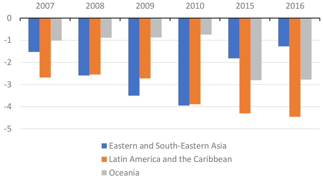
For interpretation of the statistics, if the value is shown as positive, the statistics represent an area gain while if the value is shown as negative, it represents a loss in surface area. Figure 4 shows the total mangrove area change in Eastern and South-Eastern Asia, Latin America and the Caribbean, and Oceania.
Figure 4.
Mangrove total area change (%).
Known limitations of the data are:
• The mangroves map is a global dataset, and as such, it should not be expected to achieve the same high level of accuracy everywhere as a local scale map derived through ground surveys or the use of very high spatial resolution geospatial data;
• The classification errors (in particular omission errors) typically increase in regions of Mangrove disturbance and fragmentation such as aquaculture ponds, as well as along riverine or coastal reef mangroves that form narrow shoreline fringes of a few pixels;
• In general, the mangrove seaward border is more accurately defined than the landward side where distinction between mangrove and certain wetland or terrestrial vegetation species can be unclear;
• Stripping artefacts due to Landsat-7 scan line error are present in some areas, particularly West African regions due to lack of Landsat-5 data and persistent cloud cover;
• Known data gaps in this version (v2.0) of the dataset: Aldabra island group (Seychelles); Andaman and Nicobar Islands (India); Bermuda (U.K.); Chagos Islands; Europa Island (France); Fiji (part east of Antemeridian); Guam and Saipan (U.S.); Kiribati; Maldives; Marshall Islands; Peru (south of latitude S4
3.6Global mapping and calculation of changes of water quality
The global dataset to measure water quality for SDG indicator 6.6.1 includes two lake water parameters:
1) Turbidity (TUR), and
2) an estimate of Trophic State Index (TSI).
Table 3
Trophic state index and related chlorophyll-a concentration classes [22]
| Trophic classification | Trophic State Index, CGLOPS TSI values | Chlorophyll-a ( | |
| Oligotrophic | 0 | 0 | .04 |
| 10 | 0 | .12 | |
| 20 | 0 | .34 | |
| 30 | 0 | .94 | |
| Mesotrophic | 40 | 2 | .6 |
| 50 | 6 | .4 | |
| Eutrophic | 60 | 20 | |
| 70 | 56 | ||
| Hypereutrophic | 80 | 154 | |
| 90 | 427 | ||
| 100 | 1183 | ||
Both parameters may be used to infer a particular state, or quality, of a freshwater body. Turbidity is a key indicator of water clarity, quantifying the haziness of the water and acting as an indicator of underwater light availability. Trophic State Index refers to the degree at which organic matter accumulates in the water body and is most commonly used in relation to monitor of eutrophication. Turbidity is derived from suspended solids concentration estimates and the Trophic State Index is derived from phytoplankton biomass by proxy of chlorophyll-a (Table 3). The products are mapped at a 300
Products in the period 2006–2010 are based on observations from the Envisat MERIS mission, whereas the product 2017–2020 is derived from the OLCI sensors onboard Sentinel 3. Land/water buffer maps as well as ice maps were applied to improve the accuracy of the data. EO-derived water quality parameters are intrinsically difficult to validate, as they strongly depend on the specific lake environment and suitable in-situ data for validation is lacking for most lakes. Still, the general experience of applying EO to derive water quality is that outputs tend to be in accordance with expected spatiotemporal patterns and comparing well to published numbers [21].
For the two parameters the dataset documents monthly averages as well as multi-annual per-monthly averages for the periods 2006–2010 and 2017–2020. From these time series data, a baseline reference period has been produced comprising monthly averages across the 5 years of observations for the period 2006–2010. From these five years of data, 12 monthly averages (one for each month of the year) for both trophic state and turbidity, were derived. A further set of observations are then used to calculate change against the baseline data. These observations comprise monthly data from years 2017, 2018, 2019 and 2020. The 12 monthly averages for these four years have been derived, and the deviation from the corresponding monthly multiannual baseline computed using the following equation:
For each month, the number of valid observations has been counted and the relative share of pixels falling within the following deviation ranges:
Known limitations of the data are:
• The major limiting factor in satellite-based water quality assessment is the scarcity of available in situ data to support algorithm tuning and validation. Without dedicated field campaigns, automated monitoring stations, and community data sharing arrangements, this is likely to remain a major source of product uncertainty for some years;
• Shallow lakes as well as the influence of ice/snow is suspected to add to the observed increase in turbidity levels in the high northern latitudes.
3.7Approval of the SDG indicator 6.6.1 based on EO data by UN Member States
National indicator focal points play a critical role in data flow processes acting as the single point of entry for custodian agencies to engage Member States regarding indicator monitoring and reporting. Having dedicated indicator focal points per country facilitates smooth exchanges in communication, data collection, validation and reporting, as well as dissemination of capacity building and training materials. Such national indicator focal points (also referred to as indicator technical focal points) for SDG indicator 6.6.1 may typically be one or more individuals officially nominated by the national government and may typically be from a relevant state institution such a Ministry or Department with responsibility for water management or from national statistical offices. Over the longer term, national indicator focal points can promote the ownership and uptake of indicator data within national and sub-national policy and planning processes related to the protection and management of water-related ecosystems, through the use of SDG indicator 6.6.1 data.
In March 2020, UNEP initiated direct country engagement with each of its Member State countries to obtain national approval of SDG indicator 6.6.1 EO data. National statistics per ecosystem type were sent to pre-confirmed SDG indicator 6.6.1 focal persons, SDG 6 overall focal persons, and national statistical offices. During this data outreach, UNEP had over 160 countries with confirmed national indicator focal persons. In the 33 countries where an indicator focal person was unable to be established, communications were directed to either the national SDG 6 overall focal person or the SDG national statistical office focal person, as a default approach.
The UNEP help desk for SDG indicator 6.6.1, which includes a dedicated United Nations email address for the indicator, was set up to manage the process of national data approval and respond to technical questions and queries from countries about indicator data. The indicator help desk team comprises staff within UNEP’s freshwater ecosystem unit, and technical specialists from data-providing organisations, including the European Commission’s Joint Research Centre and their partners Plymouth Marine Laboratories and Brockman, Global Mangrove Watch consortium, and DHI A/S. A no-objection approach was adopted for the national data validation.
Over 60 countries engaged with the helpdesk team throughout 2020 and raised questions on specific freshwater ecosystem data that had been shared with them for national approval. In most of these cases, all technical clarifications could be resolved. However, in some instances, countries raised technical queries on ecosystem-specific data that could not be resolved. For example, data on lake water turbidity were observed to be out of alignment with national data in Finland. This northern latitude country has a multitude of shallow water lakes, and the shallow nature of the lake water appears to influence the accuracy of turbidity measurements captured by satellite imagery. In the Netherlands, saline seawater is used within its canal and inland waterway system. These saline waters were captured as part of the national freshwater surface area data, generating an inaccurate national surface water extent data set. In eight cases, the focal point requested that one or more data series from a particular sub-indicator not to be reported as the data did not accurately represent national statistics for the same ecosystem typology, in these specific cases the specific sub-indicator data were provided to the United Nations Statistics Division with explanatory notes for the sub-indicator data not to be included in the full suite of indicator 6.6.1 national data series.
In February 2021, nationally approved data for 190 countries were submitted to the United Nations Statistics Division. Data were not available for three Small Islands Developing States. The data reported constituted annual data series starting from the year 2000 up to and including 2018 depicting changes per ecosystems type as a measure of square kilometers, percentage change from a baseline period and ecosystem area compared to overall land area. The data flow process is shown in Fig. 5.
Figure 5.
Data flow process.
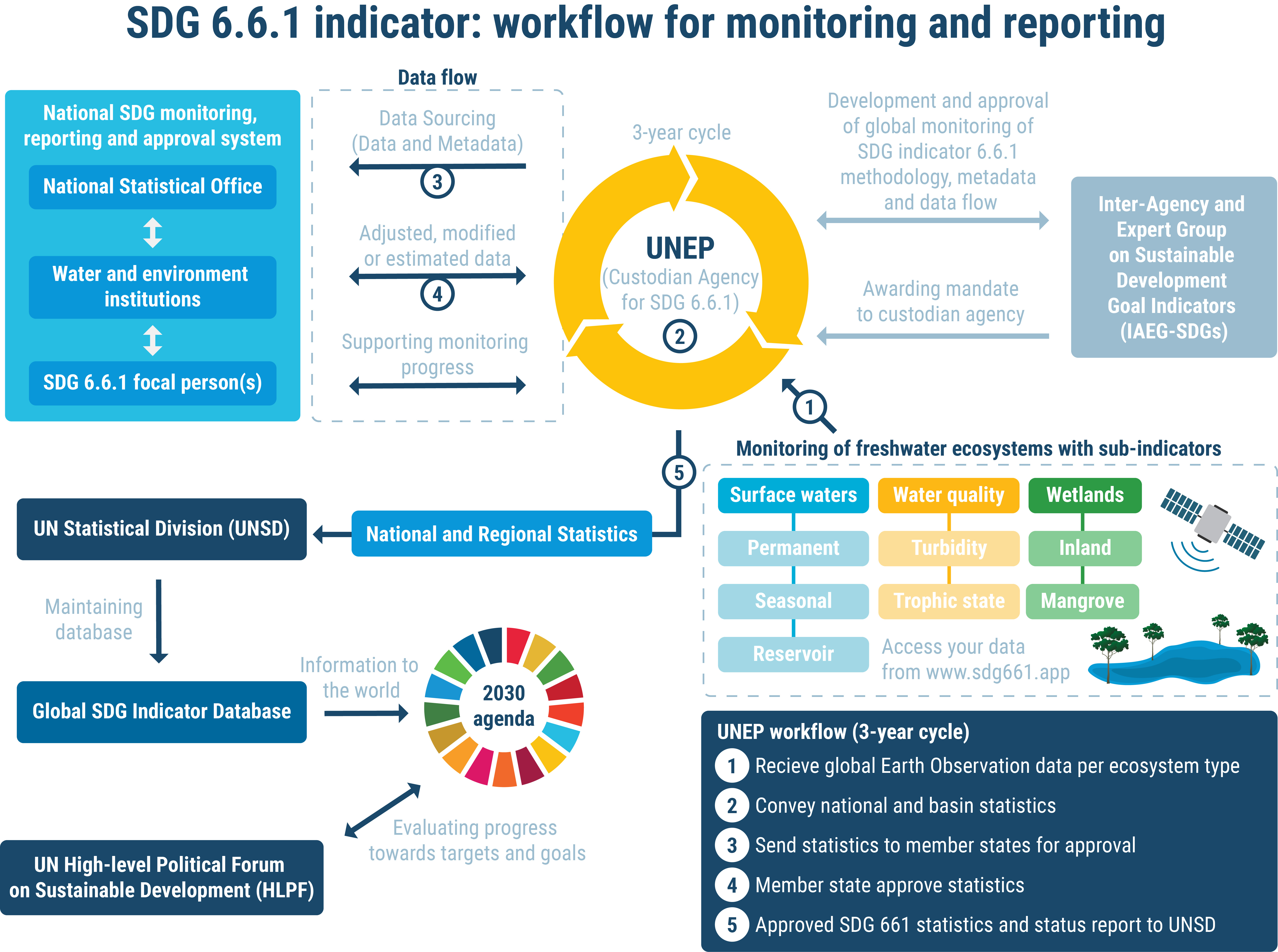
Figure 6.
Global map of river basins with observed high increase and/or decrease in surface water area during 2015–2019 compared with 2000–2019 [11].
![Global map of river basins with observed high increase and/or decrease in surface water area during 2015–2019 compared with 2000–2019 [11].](https://content.iospress.com:443/media/sji/2022/38-3/sji-38-3-sji220041/sji-38-sji220041-g006.jpg)
![Model global map of basin scorecard system [11].](https://content.iospress.com:443/media/sji/2022/38-3/sji-38-3-sji220041/sji-38-sji220041-g007.jpg)
3.8Data gaps, uptake, and moving from monitoring to action on SDG indicator 6.6.1
In summarizing the advances in using EO data to calculate water-related ecosystem extent change, it is important to note that all data come with some degree of limitations associated with data availability, but the data presented in the above sections represent a collection of globally harmonised data products for reporting on SDG indicator 6.6.1.
There exist data gaps within SDG indicator 6.6.1 for reporting under river flow and on groundwater. It is anticipated that river flow data can be modelled globally, using precipitation data and run off data correlated to in-situ measures on the ground. A global model for river flow is currently being developed and tested and is likely to be available ahead of the next round of reporting. Groundwater data remain notoriously difficult to report on for many countries.
Understanding the state of the world’s freshwater ecosystems is an essential first step to protecting and restoring them. At the same time, understanding how multiple pressures interact to cause freshwater ecosystem changes is complex. Growing populations drive changes in freshwater ecosystems through increased demand. For example, they change hydrological systems to generate local storage. Deforestation and urbanisation contribute to increased run-off, higher rates of flooding and the washing-out of nutrients and sediments which degrades water bodies. Draining inland wetlands and removing coastal mangroves lowers the capacity of these ecosystems to moderate the effects of extreme weather events and reduces freshwater habitats and biodiversity. Climate change-induced rainfall variations are altering the geographical distribution of permanent surface water. At the same time, increased temperatures may result in drought and less surface water, while also contributing to increased glacial melting and thawing of permafrost, resulting in increased surface water [11].
A particular advantage of utilising EO data to monitor changes in water is that the spatial and temporal resolution of the available data provides the opportunity to overlay or correlate these water data with other global datasets of similar spatial and temporal resolution.
In 2021, UNEP produced a global assessment report on the status of SDG indicator 6.6.1 [11]. The analysis presented in the report used river basins as a sub-national spatial scale through which it is useful to assess freshwater ecosystem trends. River basins are not only naturally connected hydrological systems defined as a physical area but also where decisions on freshwater quantity and quality can be practically assessed. River basins are also exposed to climate change, population growth and land-cover change from deforestation, urbanisation and dam and reservoir construction and it is therefore possible to assess and analyse freshwater changes in conjunction with these data which may themselves act as drivers to freshwater changes. Figure 6 shows a global map of river basins with observed high increase and/or decrease in surface water area during the period 2015–2019 compared to 2000–2019.
One approach to support countries intending to transition from monitoring into action on ecosystem protection using EO data products, is the development and application of a river basin scorecard. A scorecard approach could unite the SDG indicator 6.6.1 sub-indicator data into a combined aggregate score mapped at a river basin scale. Freshwater ecosystem changes per basin could be calculated using a weighted sum of changes in the sub indicators, with the extent of change per sub indicator corresponding to a numerical scale from 1 to 5, which are then brought together in a simple, flexible and robust traffic light scoring system (Eq. (4)):
(4)
The Freshwater Ecosystem (FWE) change score is the weighted sum of all sub-indicators (
Figure 7 provides a working example of this river basin scorecard approach mapped globally.
4.Conclusion
The use of non-traditional data sources for official statistics helps bridging data gaps and assists policy makers in addressing environmental challenges by using geospatial and EO data, coupled with advanced technologies especially in countries lacking the capacity and the required resources for in-situ monitoring and producing the data. The technological advancements through the years improved the data availability and accessibility, the data accuracy and the update frequency. At this point of time, efforts are being made to assist countries in replacing the global estimated data with national data using in-situ monitoring where financial and technological resources are available to produce these data according to the established and agreed methodology and to apply the no objection approach for publishing the globally estimated data from countries lacking the capacity to produce these data.
Despite the advantages provided by the usage of publicly available geospatial and EO data with varying resolution and high temporal revisit time for the monitoring and the protection of the environment, there are still some limitations in the full coverage, and the frequency of the update due to the resolution provided and the frequency of the images taken by the satellite used.
The availability of EO data for environmental monitoring is constantly growing and as presented in this paper EO-based information products on freshwater ecosystem are now available in high-resolution at global levels. Still, global products will inevitably tend to have a bias at the national/local level, and since the countries own the SDG monitoring and reporting there is a need to look at how national EO based monitoring can be enabled to provide more accurate national statistics and ensure ownership of data and information. However, the amount of data that is generated over most national territories makes it a daunting challenge to search, download, organize, pre-process and analyse such data using traditional desktop solutions. Online data platforms and the data cube concept has emerged as a promising solution to address the big data challenge in terms of dealing with data issues related to volume, variety and velocity. Data cubes are a time-series multidimensional (e.g., space, time, data type) stack of spatially aligned pixels used for efficient and effective access and analysis. Data cubes strengthens the connection between users and applications by facilitating management, access and use of Analysis Ready Data (ARD). In other words, data cubes allow users with limited EO background to harness large EO datasets without the fuss of dealing with file management and pre-processing – tasks which can be cumbersome and challenging even on limited datasets, but which are amplified many fold when considering time-series data at scale and where apart from scene-based pre-processing (e.g., calibration, cloud masking) multi-scene processing also needs to be considered (e.g., stitching, mosaicking, composting). Many of the countries currently leading the use of EO data at national scale have or are in the process of developing national data cubes. Still, the lion share of countries may not have the technical, human and institutional capacity nor the financial means to own and operate their own in-house monitoring service and hence a continued need to serve the global datasets and plug that information gap. Importantly, EO-based monitoring systems should not replace in-situ networks (availability of in-situ data is essential to calibrate and validate the EO-based retrieval algorithms), but may complement them, offering cost-effective solutions. EO-based monitoring and reporting represent in fact an up-scaling in space and time of the conventional field measurements and may capture the spatio-temporal variability of freshwater ecosystems more accurately than ground monitoring programs.
Acknowledgments
The authors of the article thank the following partner organisations: Joint Research Centre (JRC) of the European Commission, Google, US National Aeronautics and Space Administration (NASA), European Space Agency (ESA), Japan Aerospace Exploration Agency (JAXA), Global Mangrove Watch, DHI A/S, UNEP-DHI Centre on Water and Environment (UNEP-DHI), Aberystwyth University, Brookman Consult, and Plymouth Marine Laboratory.
References
[1] | Open Data Inventory 2020/2021 by Open Data Watch. Annual report. Available from: https://odin.opendatawatch.com/Report/annualReport2020. |
[2] | Measuring Progress: Environment and the SDGs. Nairobi. UNEP; (2021) . Available from: https://www.unep.org/resources/publication/measuring-progress-environment-and-sdgs. |
[3] | Framework for the Development of Environment Statistics (FDES 2013). New York. United Nations; (2017) . Available from: https://unstats.un.org/unsd/envstats/fdes.cshtml. |
[4] | SAS [home page on the Internet]. Available from: https://www.sas.com/en_us/insights/big-data/what-is-big-data.html. |
[5] | Group on Earth Observation [home page on the Internet]. Available from: https://www.earthobservations.org/g_faq.html. |
[6] | United Nations Committee of Experts on Global Geospatial Information Management [home page on the Internet]. Available from: https://ggim.un.org/. |
[7] | Big data for environment and agriculture statistics. Bangkok. UNESCAP; (2021) . Available from: https://www.unescap.org/sites/default/d8files/knowledge-products/SD_Working_Paper_no13_Apr2021_Big_data_for_environment_and_agriculture_statistics.pdf. |
[8] | Big data for population and social statistics. Bangkok. UNESCAP; (2021) . Available from: https://www.unescap.org/sites/default/d8files/knowledge-products/Stats_Brief_Issue29_Big_data_for_population_and_social_statistics_Apr2021.pdf. |
[9] | Millennium Ecosystem Assessment. Ecosystems and Human Well Being: Wetlands and water synthesis. Island Press, Washington DC; (2005) . |
[10] | Reid AJ, Carlson AK, Creed IF, Eliason EJ, Gell PA, Johnson PT, Kidd KA, MacCormack TJ, Olden JD, Ormerod SJ. Emerging threats and persistent conservation challenges forfreshwater biodiversity. Biological Reviews. (2019) ; 94: : 849–873. |
[11] | Progress on freshwater ecosystems: tracking SDG 6 series – global indicator 6.6.1 updates and acceleration needs. UNEP; (2021) . Available from: https://www.unwater.org/app/uploads/2021/09/SDG6_Indicator_Report_661_Progress-on-Water-related-Ecosystems_2021_EN.pdf. |
[12] | Freshwater Ecosystems Explorer [home page on the Internet]. Available from: https://www.sdg661.app/. |
[13] | Lehner B, Grill G. Global river hydrography and network routing: Baseline data and new approaches to study the world’s large river systems. Hydrological Processes. (2013) ; 27: (15): 2171–2186. Available from: doi: 10.1002/hyp.9740. |
[14] | Pekel J-F, Cottam A, Gorelick N, Belward AS. High-resolution mapping of global surface water and its long-term changes. Nature. (2016) ; 540: : 418–422. doi: 10.1038/nature20584. |
[15] | Sayre R, Noble S, Hamann S, Smith R, Wright D, Breyer S, Butler K, Van Graafeiland K, Frye C, Karagulle D, Hopkins D, Stephens D, Kelly K, Basher Z, Burton D, Cress J, Atkins K, Van Sistine DP, Friesen B, Allee R, Allen T, Aniello P, Asaad I, Costello MJ, Goodin K, Harris P, Kavanaugh M, Lillis H, Manca E, Muller-Karger F, Nyberg B, Parsons R, Saarinen J, Steiner J, Reed A. A new 30 meter resolution global shoreline vector and associated global islands database for the development of standardized ecological coastal units. Journal of Operational Oceanography. (2019) ; 12: (sup2): S47–S56. doi: 10.1080/1755876X.2018.1529714. |
[16] | Pickens AH, Hansen MC, Hancher M, Stehman SV, Tyukavina A, Potapov P, Marroquin B, Sherani Z. Mapping and sampling to characterize global inland water dynamics from 1999 to 2018 with full Landsat time-series. Remote Sensing of Environment. (2020) ; 243: : 111792. |
[17] | Tottrup C, Druce D, Tong X, Barvels E, Christensen M, Grogan K, Huber S, Crane S. The Global Wetland Extent: Towards a highresolution global-level inventory of the spatial extent of vegetated wetlands. Horsholm. DHI-GRAS; (2020) . Available from: https://files.habitatseven.com/unwater/Measuring-the-spatial-extent-of-wetlands-globally_Detailed_technical_specifications.pdf. |
[18] | Jarvis A, Reuter HI, Nelson A, Guevara E. Hole-filled SRTM for the globe Version 4, available from the CGIAR-CSI SRTM 90m Database: http://srtm.csi.cgiar.org. (2008) . |
[19] | de Ferranti J. Digital Elevation Data. Viewfinder Panoramas. Available from: http://www.viewfinderPanoramas.org/dem3.html. |
[20] | Copernicus DEM Product Handbook. Airbus; (2019) . Available from: https://spacedata.copernicus.eu/documents/20126/0/GEO1988-CopernicusDEM-SPE-002_ProductHandbook_I1.00+%281%29.pdf/40b2739a-38d3-2b9f-fe35-1184ccd17694?t=1612269439996. |
[21] | Gholizadeh MH, Melesse AM, Reddi L. A comprehensive review on water quality parameters estimation using remote sensing techniques. Sensors. (2016) ; 16: (8): 1298. Available from: doi: 10.3390/s16081298. |
[22] | Carlson. A Trophic State Index for Lakes. Limnology and Oceanography. (1977) ; 22: (2): 361–369. doi: 10.4319/lo.1977.. |


