
Using machine learning to make government spending greener
Abstract
In the face of the Triple Planetary Crisis concerning climate change, biodiversity loss, and pollution, the global community is in dire need of quantitative, data-based approaches to inform its response and guide its path towards a sustainable and equitable future. Government spending and fiscal policy are key levers in shaping this response. In order to assess the potential for using machine learning to inform policymakers’ and governments’ decision-making and spending allocation decisions based on environmental outcomes, the United Nations Environment Programme (UNEP) and the United Nations Conference on Trade and Development (UNCTAD) collaborated to produce a joint pilot study. The study uses official development assistance data (ODA) to train machine learning models to predict deforestation rates in six different countries: the Democratic Republic of the Congo, Haiti, Liberia, Madagascar, Solomon Islands, and Zambia. Initial modelling results were promising and the approach could prove to be a valuable asset to policymakers by enabling scenario analysis, where hypothetical budgets or spending allocations can be run through models trained on historical data to give insight on potential impacts on environmental indicators. Future research could be expanded to a pilot study with a national government using disaggregated budget data instead of ODA as model inputs.
1.Introduction
In 2020, the United Nations Environment Programme (UNEP) highlighted three critical planetary crises affecting the international community: climate change, biodiversity loss, and pollution [1]. An essential pillar in addressing these topics is the role of governments, in particular their fiscal policy and budgets. With targeted, green fiscal policy, governments can either minimize spending which intensifies the crises, or, better yet, support measures which actively address and mitigate them.
The aftermath of the COVID crisis was seen by many as an opportunity to build back greener [2]. While the long-term economic and environmental consequences of the pandemic remain to be seen, there is growing consensus that addressing social and economic conditions cannot be considered separately from environmental conditions [2]; policies for the former must incorporate considerations for the latter for the long-term health and sustainability of the global economy. After all, more than half of global GDP is highly or moderately dependent on nature [3]. Public and fiscal policy are some of the most immediate and impactful means of addressing social, economic, and environmental issues, yet national budgets are rarely determined or informed using systematic, quantitative analysis or scenario analysis, where the potential impacts of different spending decisions are examined using data and models.
Expanding the role of quantitative analysis in government decision-making will be key to accomplishing the long-term goal of a green, inclusive recovery and economy. Researching, promoting, and providing access to monitoring tools and methods would greatly increase the impact, accountability, and transparency of public spending [4]. Data and advanced quantitative methods could play a key role in helping guide our future decision-making [1]. This may take the form of either leveraging and extracting more insights from existing data or of making use of the ever-increasing quantities and varieties of new data being produced on a daily basis. Machine learning methodologies such as those applied in this paper have immense potential to impact and improve the public sector, but further research to assess the possibilities and address potential issues, such as the perpetuation of biases, needs to be conducted.
In this spirit and in order to bring this vision closer to reality, UNEP and the United Nations Conference on Trade and Development (UNCTAD) undertook an inter-agency collaboration to assess the feasibility of using machine learning and data-based approaches to inform spending decisions based on their potential impact on environmental indicators. The hope is that exploratory and proof of concept research such as this can serve as inspiration and a starting point for governments in utilizing new methodologies to inform their spending and budgetary decisions and efficiently allocate their scarce funds to maximize progress towards sustainable and inclusive economies and development.
The analysis used official development assistance (ODA) data to train machine learning models in predicting deforestation rates in six different countries: the Democratic Republic of the Congo, Haiti, Liberia, Madagascar, Solomon Islands, and Zambia. Initial results were promising and illustrate how machine learning could help inform spending decisions. The rest of the paper will proceed as follows. Section 2 will provide background information on the ODA and environmental situation in each of the six countries, as well as information on machine learning and the methods employed in the analysis; Section 3 will provide details of the analysis performed; Section 4 will discuss the results of the analysis; Section 5 will conclude and discuss potential ways forward.
2.Background
2.1Green spending and deforestation
Deforestation plays a critical role in the aforementioned planetary crises, as forests foster biodiverse ecosystems and combat climate change through carbon sequestration. This role, coupled with good data coverage and availability from Global Forest Watch on deforestation across the globe, made it an ideal target variable for the analysis, acting as a proxy for environment-related outcome indicators.
The goal of the analysis was to predict deforestation rates using data on spending and fiscal decisions. Lacking access to national governments’ historical and disaggregated budgets, we were limited to publicly available datasets. In this regard, ODA was an ideal proxy, comprising a completely transparent and public component of governments’ spending due to flows originating in donor countries. Furthermore, ODA flows are broken down by economic sector and environmental marker targeted [5].
Of course, ODA or government spending is not the only factor impacting deforestation rates. An all-encompassing model perfectly capturing the diverse components and their interplay affecting deforestation would be impossible to construct. However, there are characteristics which could make it more or less likely for ODA in a given country to have a greater impact on deforestation. In particular, large ODA inflows relative to gross national income (GNI) in a country increases the likelihood that a model based on ODA would be able to capture important elements affecting deforestation, underpinned by the knowledge that lower income or less economically developed economies are often tempted to exploit their natural resources and assets to act as a fiscal buffer [6].
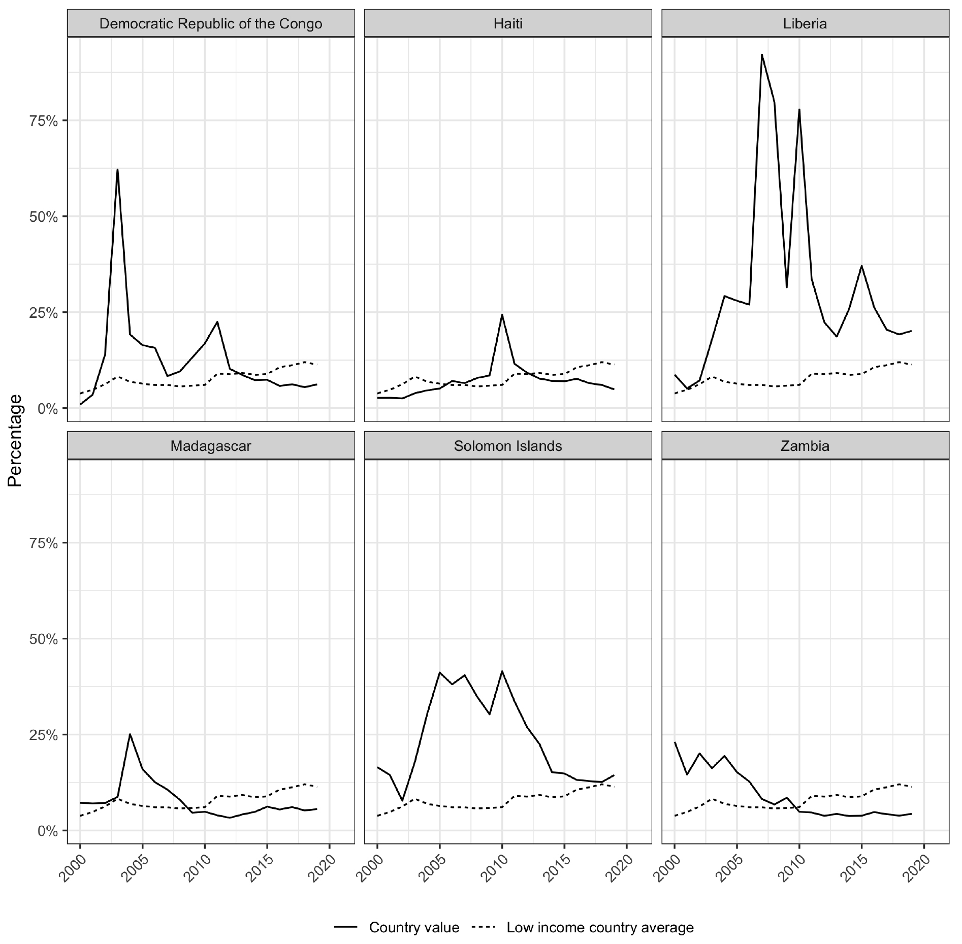
These assumptions guided the selection of the six countries examined in the analysis; each coupled high deforestation rates with elevated levels of net ODA to GNI ratios. Figures 1 and 2 show the cumulative treecover losses, in percentage, since 2000 and net ODA to GNI ratios for the six countries, respectively. Each country had lost at least seven per cent of its 2000 treecover by 2020, ranging all the way up to 24 per cent for Madagascar. Over the period from 2000 to 2019, each country also averaged at least the low income country average for net ODA as a percentage of GNI, as in the case of Haiti, ranging up to more than four times that average in the case of Liberia. The following sections will briefly explore the specific environmental and fiscal circumstances of each country.
Figure 1.
Cumulative tree cover loss since 2000.
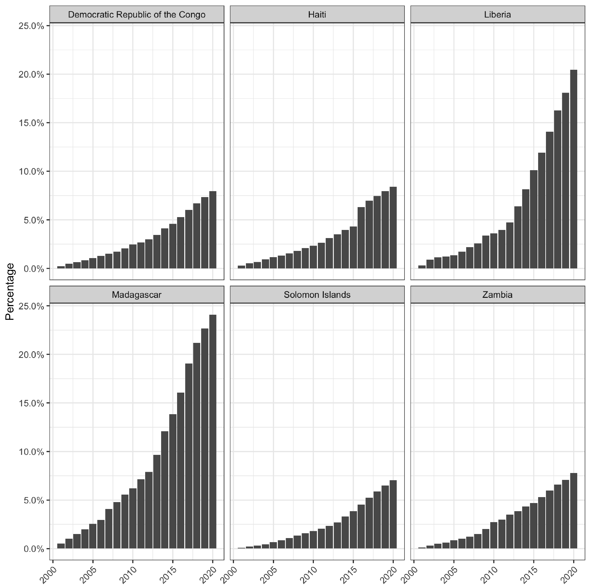
Figure 2.
Net ODA received as a percentage of GNI.
Democratic Republic of the Congo
The Democratic Republic of the Congo (DRC) is home to rich and diverse forest assets, hosting the majority of the Congo Rainforest. These teeming forests help the country count as the most biodiverse country in Africa, which illustrates the imperativeness of protecting its forest resources, as they play a crucial role in broader regional ecosystems [7]. Unfortunately, since 2000 the DRC has lost eight percent of its treecover, driven largely by agriculture, forestry, and industrial logging [8, 9]. Fuelwood gathering also plays an important role in deforestation.
Economically, the DRC is highly dependent on ODA, which averaged 13 per cent of GNI over the period from 2000 to 2019. The country has one of the lowest Human Development Indices (HDI) in the world [10] and is the eighth largest recipient of ODA in the world and fourth largest recipient in Africa [11]. Furthermore, 60 per cent of employment comes from agriculture, with one third of people affected by acute food insecurity [12, 13], increasing the likelihood that targeted ODA flows may have a substantive impact on rates of deforestation.
Haiti
Haiti is a biodiversity hotspot within the broader hotspot of the Caribbean, boasting high levels of endemic flora and fauna [14]. Unfortunately, the country has suffered from drastic rates of deforestation dating back to colonial times. Prior to the arrival of Europeans, 75 per cent of Haiti’s land was forested [15]. Since that time, industrial logging and agricultural clearances for sugar cane harvesting have taken a toll on Haiti’s forests [16]. Haiti has lost eight per cent of its treecover since 2000 alone [17]. Today, the border between Haiti and the Dominican Republic, with whom it shares the island of Hispaniola, is visible even from aerial and satellite photography due to their differing histories and paths regarding deforestation.
A primary driver of deforestation in Haiti is the demand for fuelwood, which makes up almost 80 per cent of Haiti’s primary energy supply [18, 19]. This demand is driven, in turn, by subpar electrical and power infrastructure, driving people to turn to woodfuels as alternative energy sources [20]. The situation is exacerbated by more than 60 per cent of rural land lacking legally recognized ownership documents, which disincentivizes sustainable land and agricultural practices [21].
From an ODA perspective, Haiti’s receipts as a percentage of GNI are in line with the low income country average, as evidenced in Fig. 2. The exception being 2010, when a magnitude 7 earthquake caused a large humanitarian disaster and subsequent inflow of foreign aid. ODA reached nearly 25 per cent of GNI in 2010.
Liberia
Liberia is home to most of West Africa’s remaining primary tropical forests, constituting an important part of the Guinean Forests of West Africa. In 2000, 96 per cent of Liberia was covered in natural forest [17]. However, it had lost 22 per cent of that treecover by 2020, the equivalent of 1.11 gigatonnes of carbon emissions [17]. Agriculture and mining are the primary drivers of deforestation in the country, with natural resource extraction and exploitation making up a significant portion of its economy [22].
The country is making efforts to address its alarming rate of environmental degredation, making a zero-deforestation commitment in 2014 [23]. It has additionally signed a voluntary partnership agreement with the European Union with the goal of improving lumber traceabilitiy and forest management [24], but on the ground changes remain difficult to spot [25].
Liberia averaged the highest proportion of ODA to GNI from 2000 to 2019 in the six-country sample. Two civil wars dating from 1983 to 2003 wrought destruction upon the country and spurred dramatic levels of foreign assistance in the 2000s. Since 2010, the ODA to GDP ratio has declined, but still remains well above the low income country average.
Madagascar
Madagascar is home to a unique ecosystem, with more than 80 per cent of its flora and fauna unique to the island [26]. Unfortunately, it also suffers from rampant deforestation, losing 25 per cent of its forest cover between 2000 and 2020 [17]. At current rates, deforestation and climate change could see the disappearance of the country’s eastern rainforest by 2070 [26].
As in other countries, agriculture has been the primary engine of deforestation in Madagascar. With a rapidly increasing population to feed, forests are rapidly being converted to farmland despite government efforts [27]. Poor farmers have little choice other than to turn to unsustainable agriculture practices, such as slash-and-burn [27].
Since 2000, on average, Madagascar has experienced higher ODA to GNI ratios than the low income country average, mostly driven by extremely high inflows in the 2000s. Since 2010, though still substantial, the ratio has fallen below the low income country average.
Solomon Islands
Like other countries in the analysis, the Solomon Islands are a hotbed of biodiversity in terms of both flora and fauna, counting over 3 200 indigenous plant species and a wide array of birds, mammals, and fish [28]. The country’s population is largely rural, with a large percentage relying on the country’s wildlife and natural resources for food and income [28]. Similar to Liberia, 96 per cent of the country was covered in forests in 2000, though its rate of loss since then has been lower than that of Liberia; in 2020, the Solomon Islands had lost seven per cent of its forest cover.
Commercial agriculture, especially palm oil plantations, coupled with logging and mining, are the primary drivers of deforestation in the country [28]. Timber in particular is an important industry for the country, which counts as the second largest exporter of round logs to China, posing an acute threat to the country’s forests [29, 30]. As an island nation, deforestation poses an additional threat to soil and coastline erosion and coral reefs [30].
The country’s government and the international community have made efforts to protect and properly steward the Solomon Island’s forests in recent years, for instance implementing a National Forest Inventory and joining the United Nations Programme on Reducing Emissions from Deforestation and Forest Degradation [31, 32].
The country is heavily reliant on ODA, which measured 24 per cent of GNI between 2000 and 2019, on average, though this ratio has declined since 2010.
Zambia
In 2000, about 32 per cent of Zambia’s land was under treecover, a figure which by 2020 had fallen to less than 30 per cent [17]. Historical and recent deforestation rank the country as containing the fourth largest amount of deforested area [33]. Agriculture is again the largest threat to Zambia’s remaining forests [34].
In recent years, there have been efforts to improve Zambia’s stewardship of its natural resources. For instance, in 2018, the country’s government, in partnership with the World Bank, launched a program intending to “improve sustainable land management, diversify livelihoods options available to rural commodities, including climate-smart agriculture and forest-based livelihoods, and reduce deforestation in the country’s Eastern Province” [35]. The Zambian government, with support from the United States Agency for International Development (USAID), is also working to develop a Reducing Emissions from Deforestation and Degradation strategy [33].
Prior to 2010, ODA levels as a percentage of GNI were more than twice low income country average levels, but the ratio has dropped below that average since 2010, remaining relatively stable at around five per cent.
2.2Machine learning
Machine learning is an expansive field and the information presented in this section is only a casual introduction to the topic. Specific algorithms will be discussed in further detail in the next section. For more information on machine learning in general, see [36]. For a more comprehensive background, see [37] or [38].
Machine learning refers to the study and application of algorithms whose crucial characteristic is the ability to improve their predictive performance automatically through the use of data. I.e., no human has to explicitly program or give instructions to the algorithm in order for it to produce its predictions or output. This learning and improvement process is referred to as “training” the model using existing or historical data. Machine learning is broadly generalizable into two areas: supervised learning and unsupervised learning. Supervised learning refers to algorithms and applications where both model inputs and outputs are provided to the model in training. That is, the output of the model is an existing variable with data available at the time of training. An example of a supervised machine learning application would be predicting sales of a company based on its advertisement spending. Unsupervised learning refers to the situation where the target variable is unknown or undefined. This paper is concerned with supervised machine learning, as the application has a well-defined target variable, explained in Section 3.
The first step in a supervised machine learning application is defining and gathering input and output variables. Input variables are the data the model will use to try and predict the output variable. The output, or target variable, is the variable of interest. The model is then trained on data where both the input and output variables are present. In this way, the model can establish the relationship between input and output. The ultimate goal is to generate predictions of the output variable in cases where its value is not known. This is referred to as inference. However, before the inference step, it is important to assess the performance of the model to make sure that it can generate good predictions. For this, it is necessary to test the model and generate predictions on input data where the output is known. This should not be done on the same data the model was trained on, however. This can lead to the issue of overfitting, where a machine learning model may pick up on noise in the data and subsequently produce very accurate predictions on data it was trained on, but generalize very poorly to new data it has not seen before. To ensure against this, the model is typically tested on a test set, consisting of data the model has never seen before, i.e., data it was not trained on. In the test set, both input and output variables are present. In this way, the test input data can be used to generate predictions which can then be compared with the actual values of the output variable. Good accuracy between these test predictions and the actual values can then give a better indication of the model’s performance.
This process is perhaps best clarified by way of example. Say a company is looking to predict its revenues based on its advertisement spends. It has three advertisement channels, TV, radio, and online. It has five years of monthly data on how much it spends on each of these channels. These are the input variables. The output variable is monthly revenue, for which it also has the same five years of monthly data as the input variables. Keeping in mind that it needs test data to assess its model on, it sets aside the last year’s worth of data for testing. This 80-20 per cent split of training and test data is a commonly used rule of thumb ratio in machine learning. It then trains a model using the first four years’ worth of data, where the algorithm automatically determines the relationship between the input and output variables. The company then gives the trained model the last year’s input data, generating predictions for monthly revenue. These predictions are compared with the actual monthly revenue for the last year. If these predictions are sufficiently accurate, the company can finalize their model and begin using it for inference. With their trained model, they can now do things like scenario analysis, where they see how different advertisement allocations affect revenue in order to maximize the expected return of their spending, and revenue forecasting. For instance, if they have a good idea of the advertising budget available to them over the next year, they can then generate a forecast of revenues based on those figures. This is just one example of a machine learning application, but this approach can be generalized to many different situations.
3.Empirical analysis
3.1Data
Data for the analysis came from two principal sources: the Organisation for Economic Co-operation and Development (OECD) for information on ODA and aid activities, and Global Forest Watch for information on deforestation rates. Two separate series were collected by country from the OECD: ODA by economic sector [39], and aid activities targeting Global Environmental Objectives [40], a.k.a., aid activities by Rio Marker [5]. From Global Forest Watch, the ”global annual tree cover loss” series was used [17]. All series were published at an annual frequency and transformed to year-over-year growth rates. Data were transformed to growth rates for two reasons. First, to provide a clearer semantic interpretation of the data and improve comparability and interpretation across countries. Data in hectares needs to be contextualized to each individual country to be able to be understood. Is predicted deforestation of 50 000 hectares a lot or a little? For a country like St. Vincent and the Grenadines, this is a massive amount of deforestation, greater in fact than the size of the entire country, while for a country like Brazil, this represents less than 0.005 per cent of its land area. Data in hectares needs to be contextualized not only across countries, but also temporally. 50 000 hectares of deforestation is not a large number relative to the size of Brazil, but how does this compare to last year? Is the figure moving up or down, by how much? The growth rate transformation addresses both of these aspects. Second, the transformation improves the performance of many machine learning approaches by scaling all input and output variables to a smaller range. Hectares and dollars can occupy ranges from thousands to millions or billions, but growth rates tend to be much more constrained, rarely extending much beyond
3.2Methodologies
Gradient boost
Two machine learning methodologies were used in modelling deforestation as a function of ODA and aid spending: gradient boosted trees and long short-term memory artificial neural networks. Gradient boosted trees is an ensemble machine learning algorithm that builds off the results of several simpler decision tree models. A decision tree works by having all data start in one group at the root of the tree, and then splitting the data into groups at different nodes depending on the data’s features and the information gain from the split. The new groups are then split further on more detailed information, and so on until either all observations have been separated or until a pre-determined number of splits. For more information on decision trees, see [42] or [43].
Individual decision trees are generally not very performant and prone to issues like overfitting. However, they are often used as the base for ensemble methodologies, as with gradient boosted trees. The approach sequentially combines individual decision trees. Each subsequent addition is then trained to reduce the errors of the previous iteration. By combining multiple decision trees in this manner, the model can achieve results far superior to those of any individual decision tree. See [44] for more information on the topic. Gradient boosted trees are one of the most popular machine learning methodologies employed for a variety of applications [45] and have been shown to outperform linear models in time series prediction applications such as this one [46], hence their selection for the analysis.
Long short-term memory artificial neural networks (LSTM)
LSTMs are a variant of artificial neural network (ANN). Over the past decade, ANNs have garnered much interest due to their impressive performance in applications such as image recognition, autonomous driving, and natural language processing. ANNs are composed of interconnected layers of nodes. These layers receive input, transform that input by multiplying it by coefficients and running it through activation functions, before finally generating an output or prediction. Coefficients are randomized initially but are then adjusted via a process called back propagation. Back propagation involves defining a cost function, calculating gradients with respect to this function, and then adjusting the coefficients in the direction of minimizing error. In a feedforward multilayer perceptron (MLP), the simplest type of ANN, information flows through this network unidirectionally, from beginning to end. See [47] or [48] for more information on ANNs.
The unidirectional nature of feedforward ANNs means they are not always best-suited to deal with information with a temporal element. Recurrent neural networks (RNN) address this issue by introducing feedback loops to the network architecture. This makes them well-suited to applications with a time element, such as speech processing. For more information on RNNs, see [49] or [50]. RNNs can have trouble modelling long term temporal dependencies due to the issue of vanishing or exploding gradients [51]. LSTMs solve this issue by introducing a memory cell, along with an input, output, and forget gate. Gradients are subsequently able to travel through the network unchanged, allowing the LSTM to preserve longer term dependencies than RNNs. For more information on the architecture of LSTMs, see [52] or [53]. LSTMs have been shown to perform well in economic applications, such as in nowcasting global trade or US GDP [54, 55].
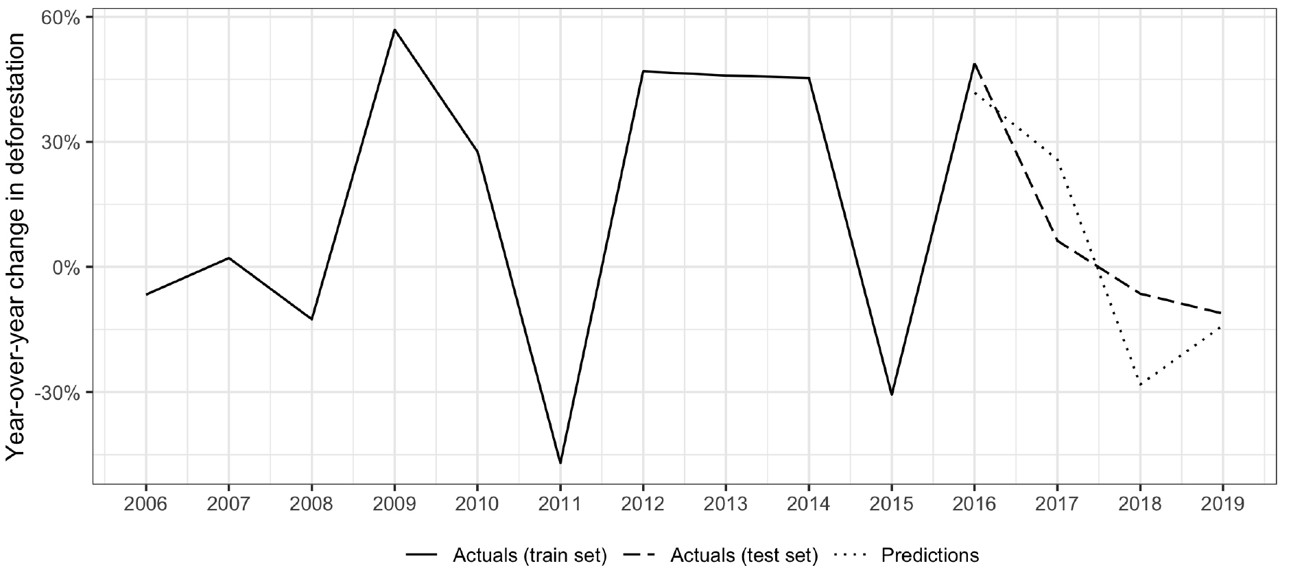
Figure 3.
Year-over-year deforestation rates in the Democratic Republic of the Congo. Note: results shown using the LSTM algorithm and ODA by economic sector input variables.
3.3Model training
In order to train and assess the models, the data were split into a train and test set. The train set consisted of data dating from 2006 to 2015, while the test set dated from 2016 to 2019. The logic of having a train and test set was to ensure the robustness of the models. A model may perform well on data it has been trained on, but may generalize poorly to new, unseen data. By evaluating the models on the test set, we can be sure that the model is not overfit to the train data and can perform adequately into the future on new data.
The test set was also used to determine hyperparameters. Hyperparameters are parameters which determine the macrostructure of a machine learning algorithm. This differs from the model’s coefficients, which are determined in the course of training or fitting the model to the data. Hyperparameters are set before a model is trained. In the case of a simple decision tree, hyperparameters may correspond to characteristics such as the max depth of the tree, i.e., the number of splits a tree can have. This can be unlimited, where splitting continues until all observations reside by themselves on a unique leaf, or can be limited to just two in the extreme, where the initial data is split into just two separate groups. Depending on the algorithm, hyperparameters can have a large impact on the predictive performance of a model. As such, they often need to be tuned. That is, define a cost function, such as mean absolute error (MAE) for a regression application, then train the model with various combinations of hyperparameters, and finally assess performance based on the cost function. The hyperparameters of the best-performing model are then used for the final model. In the ideal case, the train set is further split into a validation set for determining hyperparameters, but due to the low number of observations available in the data and the illustrative nature of the analysis the test set was used here.
In terms of input variables, three separate sets of variables were examined. The first corresponded to including only ODA by economic sector; the second to aid activities by Rio Marker; the third to the combination of both previous sets of variables. The best-performing models in terms of MAE and root mean square error (RMSE) for each country are presented in the next section.
4.Results and interpretation
Table 1 displays MAE and RMSE of each country on the test set, while Figs 3–8 display the modelling results for each of the six countries graphically. From Table 1 we can see that the model for Liberia obtained the best performance, while that for Haiti obtained the worst. In the case of Haiti, there is a reason for the poor performance which is discussed in the commentary for Fig. 4. Commentary for the results of each country follows.
Table 1
MAE and RMSE on the test set, by country
| Country | MAE | RMSE | |
|---|---|---|---|
| 1 | Democratic Republic of the Congo | 0.13 | 0.15 |
| 2 | Haiti | 1.45 | 2.11 |
| 3 | Liberia | 0.07 | 0.08 |
| 4 | Madagascar | 0.15 | 0.17 |
| 5 | Solomon Islands | 0.16 | 0.20 |
| 6 | Zambia | 0.12 | 0.13 |
Figure 4.
Year-over-year deforestation rates in Haiti. Note: results shown using the gradient boost algorithm and ODA by economic sector input variables.
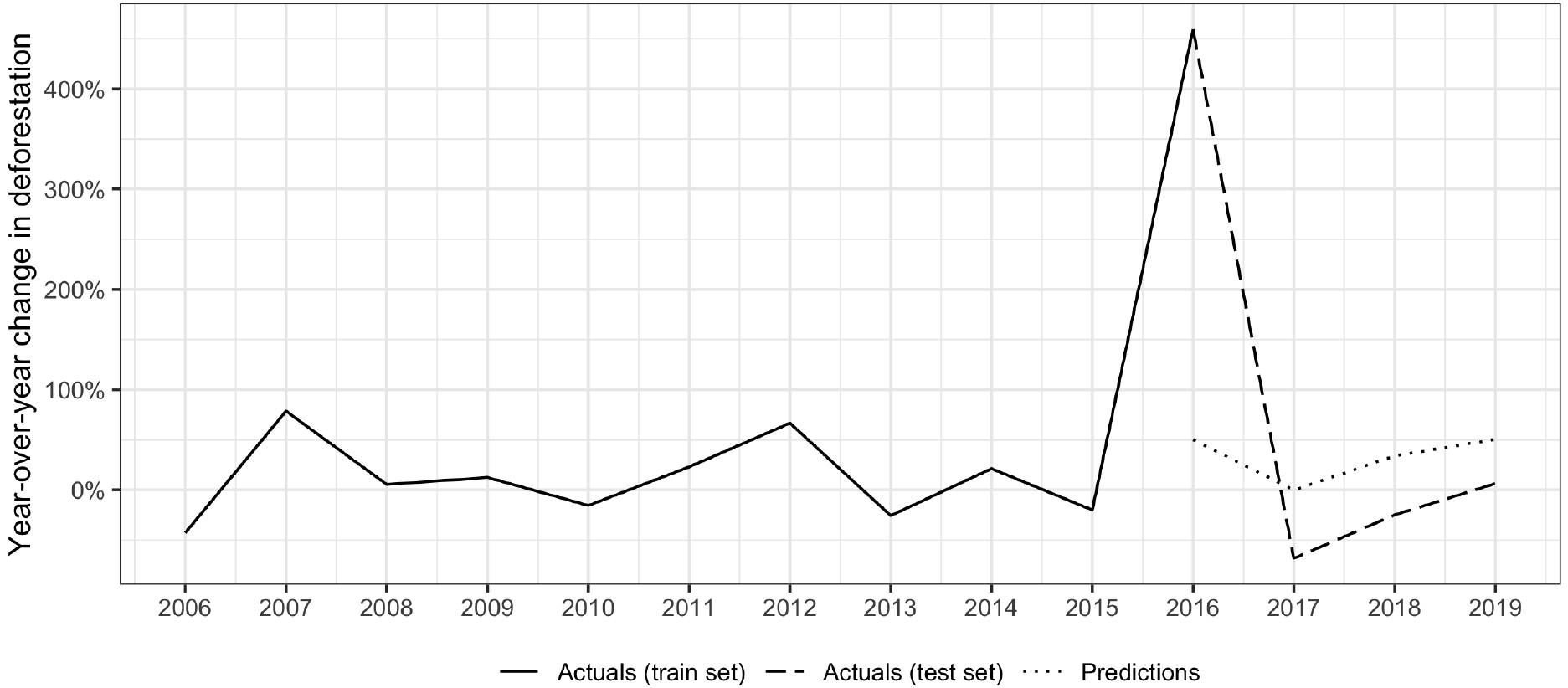
Figure 5.
Year-over-year deforestation rates in Liberia. Note: results shown using the gradient boost algorithm and aid activities by Rio Marker input variables.
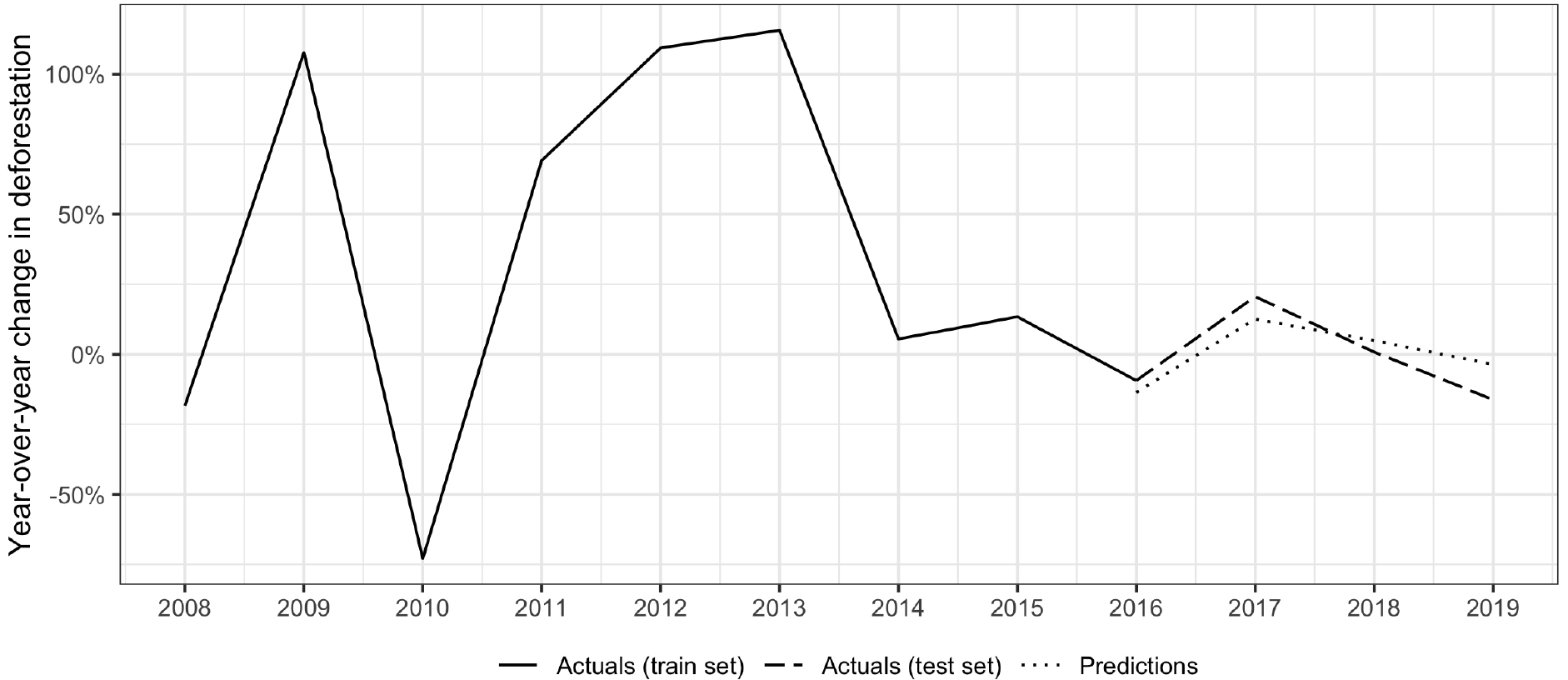
Figure 6.
Year-over-year deforestation rates in Madagascar. Note: results shown using the gradient boost algorithm and aid activities by Rio Marker input variables.
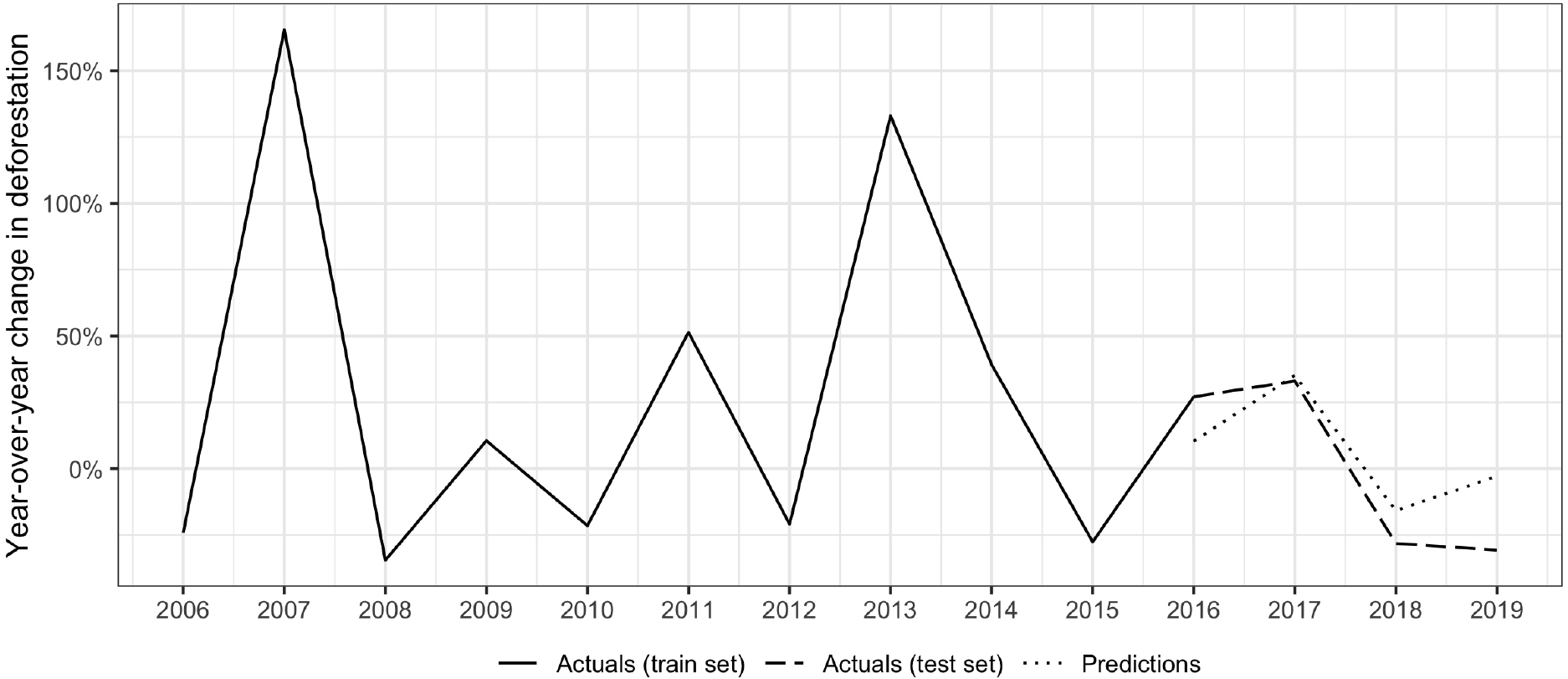
Figure 7.
Year-over-year deforestation rates in Solomon Islands. Note: results shown using the LSTM algorithm and ODA by economic sector input variables.
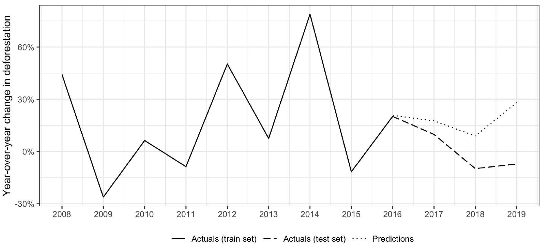
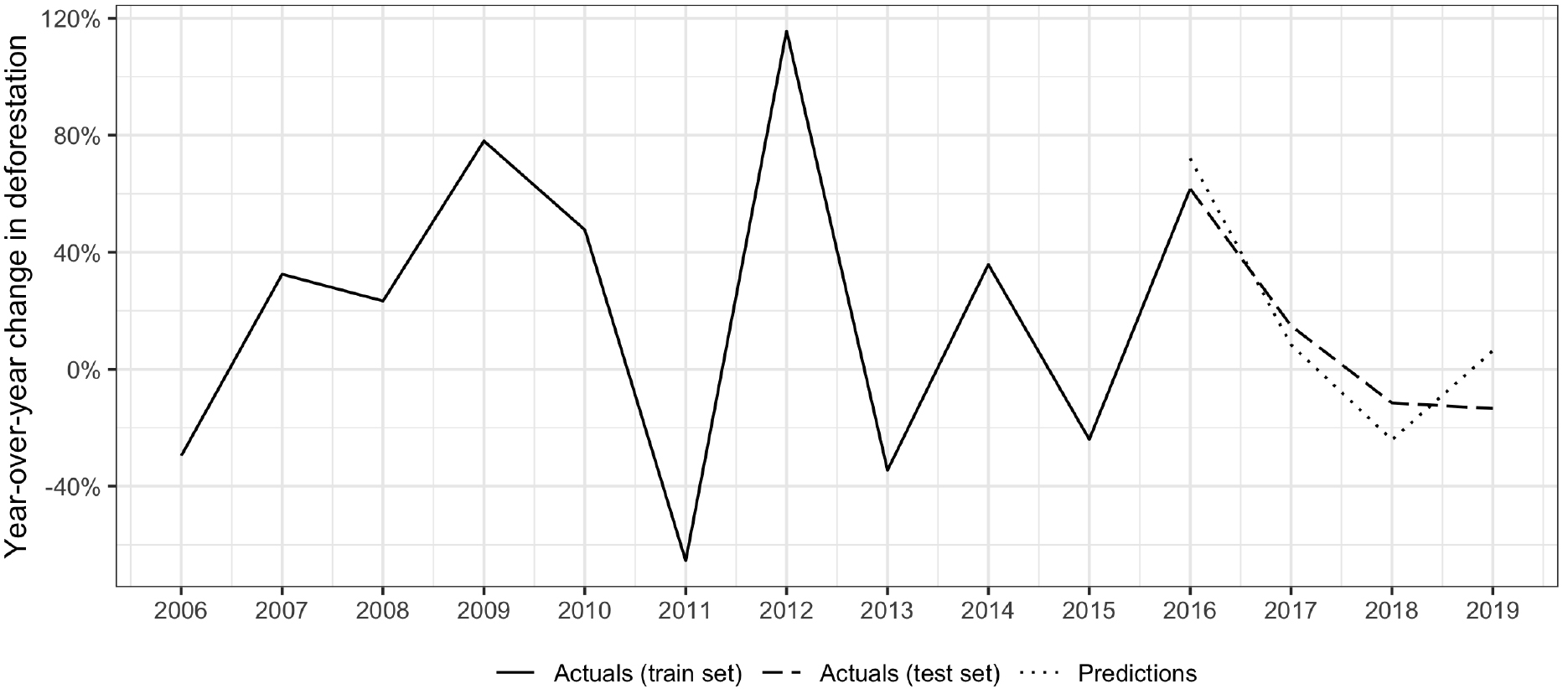
Figure 8.
Year-over-year deforestation rates in Zambia. Note: results shown using the gradient boost algorithm and both ODA by economic sector and aid activities by Rio Marker input variables.
For the Democratic Republic of the Congo, an LSTM model taking economic sector-disaggregated ODA data as inputs displayed promising predictive potential. 2016 and 2019 predictions were quite accurate, with predictions just seven and three percentage points off actuals, respectively. Rates for 2017 and 2018, however, were relatively over and under-estimated, respectively. The overall downward trend in deforestation rates between 2016 and 2019 was accurately captured by the model.
In 2016, Haiti was hit by Hurricane Matthew, a Category 5 hurricane and the strongest to hit the country since 1964. Unfortunately, the storm’s effects were even worse than in 1964 due to the effects of extensive deforestation and soil erosion, leading to more than 500 deaths [56]. Ultimately, factors linked to the storm led to record rates of deforestation in 2016, clearly visible in Fig. 4.
Lacking variables capturing the impacts of natural disasters on deforestation, the model struggled mightily with its 2016 prediction, as might be expected. In subsequent years, it continued to overestimate rates of deforestation, potentially indicating that much of the deforestation that may have happened from 2017–2019 was brought forward to 2016. Despite high errors in absolute levels of deforestation growth rates, the model remained quite accurate in capturing relative year to year changes in rates.
The model for Liberia slightly underestimated deforestation growth rates in 2016 and 2017, by four and eight percentage points, respectively, while slightly overestimating them in 2018 and 2019, by four and 13 percentage points, respectively. Again, the model was able to capture relative trends in the test period, including a relative spike in rates in 2017 and a subsequent tapering off thereafter.
The model for Madagascar underestimated rates by 17 percentage points in 2016, but was remarkably accurate for 2017, predicting values just two percentage points different from actual observations. Predictions in 2018 and 2019 both overestimated rates, especially in 2019, where they were 28 percentage points higher than actuals.
The model for Solomon Islands struggled in all years but 2016, where its predictions were off by a mere 60 basis points. Thereafter, however, it produced predictions consistently higher than actuals, with an increasing error over time. This positive bias indicates that there may be an important component driving deforestation not captured in the model.
The model for Zambia was quite accurate for 2016 and 2017, its predictions differing from actuals by only 10 percentage points and seven percentage points, respectively. This error rose to 13 percentage points in 2018 and 20 percentage points in 2019. Despite 2019’s relatively large error, the model was able to successfully capture 2016’s increase in rates and decline in subsequent years.
5.Conclusion
The exploratory analysis conducted for this paper demonstrates the potential and possibilities that machine learning could provide in understanding interdependencies between spending decisions and environmental outcomes. It could become a key component of evidence-based policy design and budgeting and help policymakers allocate funds in an optimal manner to achieve both socio-economic and environmental goals.
Despite limitations in the pilot dataset, including a training set consisting of only 10 years of annual data, modelling was able to produce surprisingly accurate predictions of yearly deforestation growth rates in several countries, such as in Liberia and Zambia. For others, despite large errors in actual predicted values, trends were still accurately captured, such as in Haiti and the Democratic Republic of the Congo. These are promising indications that, with additional data and research, similar models could be used by policymakers and budget planners to help inform their decision-making.
While the predictions of a machine learning model should never be taken as fact, they could prove immensely useful in running scenario analyses, where different provisional budgets could be run through a model trained on historical budgets to gain insights on the directionality and magnitude of effects on various environmental and socio-economic indicators. Machine learning could become yet another tool in policymakers’ arsenal to make better informed decisions on how spending allocations could impact the environment. With more insight to how present and future spending decisions impact various environmental indicators, policymakers could more accurately forecast the future environmental state of their countries and preempt and adapt to current and future challenges, rather than react.
A more comprehensive pilot study in collaboration with a national government using historical budget data would serve as a valuable next step in exploring this innovative method of transforming public finance decision-making.
Acknowledgments
The author would like to thank Himanshu Sharma for his valuable feedback, guidance, and facilitation, and Ryan Maia for his indispensable initiative, research, and coordination.
References
[1] | Andersen I. The triple planetary crisis: Forging a new relationship between people and the earth; (2020) . Available from: https://www.unep.org/news-and-stories/speech/triple-planetary-crisis-forging-new-relationship-between-people-and-earth. |
[2] | Stone S, Kim JA, Sharma H. Green Fiscal Policies For A Sustainable And Resilient COVID-19 Recovery; (2020) . Available from: https://greenfiscalpolicy.org/blog/green-fiscal-policies-for-a-sustainable-and-resilient-covid-19-recovery/. |
[3] | Forum WE. Half of World’s GDP Moderately or Highly Dependent on Nature, Says New Report; (2020) . Available from: https://www.weforum.org/press/2020/01/half-of-world-s-gdp-moderately-or-highly-dependent-on-nature-says-new-report/. |
[4] | UNEP. Are we on track for a green recovery? Not Yet; (2021) . Available from: https://www.unep.org/news-and-stories/press-release/are-we-track-green-recovery-not-yet. |
[5] | OECD. OECD DAC Rio Markers for Climate: Handbook. OECD; (2016) . Available from: https://www.oecd.org/dac/environment-development/Revised%20climate%20marker%20handbook_FINAL.pdf. |
[6] | UNEMG. Regional Nexus Approaches to Building Back Better: Outcome Doucment; (2021) . Available from: https://unemg.org/wp-content/uploads/2021/05/Defining-Green-Recovery-ND_Outcome-Report_FINAL.pdf. |
[7] | UNEP. The Democratic Republic of the Congo: Post-Conflict Environmental Assessment United Nations Environment Programme Synthesis for Policy Makers. Nairobi: UNEP; (2011) . Available from: https://postconflict.unep.ch/publications/UNEP_DRC_PCEA_EN.pdf. |
[8] | Ickowitz A, Slayback D, Asanzi P, Nasi R. Democratic Republic of the Congo: A synthesis of the current state of knowledge. Nairobi: Center for International Forestry Research; (2015) . Available from: https://www.cifor.org/knowledge/publication/5458/. |
[9] | Pendrill F, Persson UM, Godar J, Kastner T, Moran D, Schmidt S, et al. Agricultural and forestry trade drives large share of tropical deforestation emissions. Global Environmental Change. (2019) ; 56: : 1–10. Available from: https://www.sciencedirect.com/science/article/pii/S0959378018314365. |
[10] | Capacity4dev. Democratic Republic of the Congo; (2022) . Available from: https://europa.eu/capacity4dev/public-environment-climate/wiki/democratic-republic-congo. |
[11] | OECD. ODA to Developing Countries – Summary; (2021) . Available from: https://www.oecd.org/dac/financing-sustainable-development/development-finance-topics/Developing-World-Development-Aid-at-a-Glance-2021.pdf. |
[12] | ITA. Democratic Republic of the Congo – Country Commercial Guide; (2021) . Available from: https://www.trade.gov/country-commercial-guides/democratic-republic-congo-agriculture. |
[13] | ReliefWeb. Scale of acute hunger in the Democratic Republic of the Congo “staggering”, FAO, WFP warn; (2021) . Available from: https://reliefweb.int/report/democratic-republic-congo/scale-acute-hunger-democratic-republic-congo-staggering-fao-wfp#:∼:text=The%20number%20of%20people%20affected,Phase%20Classification%20(IPC)%20analysis. |
[14] | USAID, Service UF. Haiti Biodiversity and Tropical Forest Assessment; (2010) . Available from: https://pdf.usaid.gov/pdf_docs/PA00T2T6.pdf. |
[15] | Velasquez-Manoff M. After the earthquake: Haiti’s deforestation needs attention; (2010) . Available from: https://projects.ncsu.edu/project/amazonia/CSM_20Jan2010.pdf. |
[16] | Lindskog P. From Saint Domingue to Haiti: Some consequences of European colonisation on the physical environment of Hispaniola. Caribbean Geography. (1998) Sep; 9: (2): 71–86. Place: Kingston Publisher: University of the West Indies. Available from: https://www.proquest.com/scholarly-journals/saint-domingue-haiti-some-consequences-european/docview/232108976/se-2?accountid=28970. |
[17] | Watch GF. Global Deforestation Rates & Statistics by Country; (2022) . Available from: https://globalforestwatch.org/dashboards/. |
[18] | Ghilardi A, Bailis R. Potential environmental benefits from woodfuel transitions in Haiti: Geospatial scenarios to 2027. Enviorn Res Lett. (2018) ; 13: (035007). _eprint: https:// www.science.org/doi/pdf/10.1126/science.aaa8415. Available from: https://www.science.org/doi/abs/10.1126/science.aaa8415. |
[19] | Sharples C, Erickson-Davis M. If Current Deforestation Rates Continue, Haiti May Lose its Forests within Two Decades; (2018) . Available from: https://psmag.com/environment/haiti-is-set-to-lose-its-forests-in-twenty-years. |
[20] | Michel G, Kendall MD. Charcoal Production through Distillation of Wood, perhaps the Key to the Deforestation of Haiti. Journal of Haitian Studies. (2013) ; 19: (1): 282–287. Publisher: Center for Black Studies Research. Available from: http://www.jstor.org/stable/24344223. |
[21] | USAID. Haiti; (2021) . Available from: https://www.land-links.org/country-profile/haiti-2/#1528915719453-17c37d2f-36cc. |
[22] | Liberia. Liberia’s National Biodiversity Strategy and Action Plan. Liberia; (2004) . Available from: https://www.cbd.int/doc/world/lr/lr-nbsap-01-p1-en.pdf. |
[23] | Authority LFD. National Strategy for Reducing Emissions from Deforestation and Forest Degradataion (REDD+) in Liberia; (2016) . Available from: http://extwprlegs1.fao.org/docs/pdf/lbr179067.pdf. |
[24] | Flegt E. The Liberia-EU Voluntary Partnership Agreement; (2017) . Available from: https://www.euflegt.efi.int/background-liberia. |
[25] | Pacheco P, Mo K, Dudley N, Shapiro A, Aguilar-Amuchastegui N, Ling PY, et al. Deforestation Fronts: Drivers and Responses in a Changing World. Gland, Switzerland: WWF; (2021) . Available from: olab.research.google.com/drive/1ZiH932TnvXbxSbG-5ovMpDhXJd0gno9s#scrollTo=5MJr71ylia2r. |
[26] | The Graduate Center C. Climate change and deforestation could decimate Madagascar’s rainforest habitat by 2070; (2020) . Available from: www.sciencedaily.com/releases/2020/01/200102143425.htm. |
[27] | Clark M. Deforestation in Madagascar: Consequences of Population Growth and Unsustainable Agricultural Processes; (2012) . |
[28] | CBD. Solomon Islands – Main Details; (2020) . Available from: https://www.cbd.int/countries/profile/?country=sb. |
[29] | Hunt L. Logging Ravaging the Solomon Islands’ Forests; (2019) . Available from: https://asiatimes.com/2019/05/logging-ravaging-the-solomon-islands-forests/. |
[30] | Government SI. A Brief Report on the State of Biodiversity for Food and Agriculture In Solomon Islands; (2016) . Available from: https://www.fao.org/3/CA3432EN/ca3432en.pdf. |
[31] | UN-REDD. Solomon Islands National Programme Overview; (2022) . Available from: https://www.unredd.net/support/support-mechanisms/national-programmes/solomon-islands.html. |
[32] | Community P. REDD+ breathes new life into Pacific forests; (2021) . Available from: https://www.spc.int/updates/blog/2021/03/redd-breathes-new-life-into-pacific-forests. |
[33] | USAID. Zambia: Environment; (2022) . Available from: https://www.usaid.gov/zambia/environment. |
[34] | Kalinda T, Bwalya S, Munkosha J, Siampale A. An Appraisal of Forest Resources in Zambia using the Integrated Land Use Assessment (ILUA) Survey Data 1. Research Journal of Environmental and Earth Sciences. (2013) Oct; 5: : 619–630. |
[35] | Bank W. Zambia Takes the Keys Away from ‘Drivers’ of Deforestation; (2018) . Available from: https://www.worldbank.org/en/news/feature/2018/03/02/zambia-takes-the-keys-away-from-drivers-of-deforestation. |
[36] | Jordan MI, Mitchell TM. Machine learning: Trends, perspectives, and prospects. Science. (2015) ; 349: (6245): 255–260. _eprint: https://www.science.org/doi/pdf/10.1126/science.aaa8415. Available from: https://www.science.org/doi/abs/10.1126/science.aaa8415. |
[37] | Mohri M, Rostamizadeh A, Talwalkar A. Foundations of Machine Learning. Adaptive Computation and Machine Learning series. MIT Press; (2012) . Available from: https://books.google.co.uk/books?id=maz6AQAAQBAJ. |
[38] | James G, Hastie T, Tibshirani R, Witten D. An introduction to statistical learning: with applications in R. New York: Springer, [2013] ©2013; (2013) . Available from: https://search.library.wisc.edu/catalog/9910207152902121. |
[39] | OECD. ODA by sector (indicator); (2022) . Available from: doi: 10.1787/a5a1f674-en. |
[40] | OECD. Aid activities targeting Global Environmental Objectives (CRS); (2022) . Available from: https://stats.oecd.org/Index.aspx?DataSetCode=RIOMARKERS. |
[41] | Ciaburro G, Venkateswaran B. NEURAL NETWORKS WITH R; (2017) . |
[42] | Patel H, Prajapati P. Study and analysis of decision tree based classification algorithms. International Journal of Computer Sciences and Engineering. (2018) Oct; 6: : 74–78. |
[43] | scikit learn. 1.10. Decision Trees; (2021) . Available from: https://scikit-learn.org/stable/modules/tree.html. |
[44] | Natekin A, Knoll A. Gradient boosting machines, a tutorial. Frontiers in Neurorobotics. (2013) ; 7. Available from: https://www.frontiersin.org/article/10.3389/fnbot.2013.00021. |
[45] | Boehmke B. Gradient Boosting Machines; (2018) . Available from: http://uc-r.github.io/gbm_regression. |
[46] | Soybilgen B, Yazgan E. Nowcasting US GDP Using Tree-Based Ensemble Models and Dynamic Factors. Computational Economics. (2021) Jan; 57: (1): 387–417. Available from: doi: 10.1007/s10614-020-10083-5. |
[47] | Sazli M. A brief review of feed-forward neural networks. Communications, Faculty Of Science, University of Ankara. (2006) ; 50: : 11–17. |
[48] | Singh R, Prajneshu. Artificial Neural Network Methodology for Modelling and Forecasting Maize Crop Yield. Agricultural Economics Research Review. (2008) ; 21. |
[49] | Dematos G, Boyd MS, Kermanshahi B, Kohzadi N, Kaastra I. Feedforward versus recurrent neural networks for forecasting monthly japanese yen exchange rates. Financial Engineering and the Japanese Markets. (1996) Feb; 3: (1): 59–75. Available from: doi: 10.1007/BF00868008. |
[50] | Stratos K. Feedforward and recurrent neural networks; (2020) . Available from: http://www1.cs.columbia.edu/∼stratos/research/neural.pdf. |
[51] | Grosse R. Lecture 15: Exploding and Vanishing Gradients; (2017) . Available from: http://www.cs.toronto.edu/∼rgrosse/courses/csc321_2017/readings/L15%20Exploding%20and%20Vanishing%20Gradients.pdf. |
[52] | Brownlee J. Deep Learning for Time Series Forecasting: Predict the Future with MLPs, CNNs and LSTMs in Python. Machine Learning Mastery; (2018) . Available from: https://books.google.ch/books?id=o5qnDwAAQBAJ. |
[53] | Chung J, Güleehre C, Cho K, Bengio Y. Empirical Evaluation of Gated Recurrent Neural Networks on Sequence Modeling. CoRR. 2014; abs/1412.3555. _eprint: 1412.3555. Available from: http://arxiv.org/abs/1412.3555. |
[54] | Hopp D. Economic Nowcasting with Long Short-Term Memory Artificial Neural Networks (LSTM). UNCTAD; (2021) . 62. Available from: https://unctad.org/system/files/official-document/ser-rp-2021d5_en.pdf. |
[55] | Hopp D. nowcasting_benchmark; (2022) . Available from: https://github.com/dhopp1/nowcasting_benchmark. |
[56] | Reid K. 2016 Hurricane Matthew: Facts, FAQs, and how to help; (2018) . Available from: https://www.worldvision.org/disaster-relief-news-stories/2016-hurricane-matthew-facts. |

