Poverty mapping in Latin America: ECLAC experiences on small area estimation
Abstract
Poverty mapping is a valuable tool for governments and international organizations to identify the geographical areas and population groups that are most deprived or vulnerable. This approach can lead to designing and monitoring development policies more effectively. This article presents the recent experience of the Statistics Division of the UN Economic Commission for Latin America and the Caribbean (ECLAC) in using Small Area Estimation (SAE) methods to combine information from household surveys, censuses and satellite imagery to deliver poverty estimates at the provincial and municipal levels, which could not be attained using the household surveys alone.

1.Introduction
Most Latin American and Caribbean countries regularly implement nationally representative household surveys to measure living conditions indicators, including poverty and income inequality. These surveys can generally be disaggregated geographically by urban and rural areas and the first-level administrative division (i.e. departments, provinces or regions). However, when it comes to obtaining a more dissagregated direct estimation of such indicators, results are subject to lower levels of accuracy and precision, which might be below the established quality criteria for their use. Small Area Estimation (SAE) techniques allow obtaining such disaggregated estimates while improving inference quality.
This article presents the recent experience of the Statistics Division of the United Nations Economic Commission for Latin America and the Caribbean (ECLAC) in applying SAE techniques to estimate geographically disaggregated poverty indicators based on household disposable income in seventeen (17) countries in Latin America. The results show a significant improvement in the precision of FGT-family indicators for geographical areas where the surveys do not attain adequate representativeness.
ECLAC regularly produces standardized national estimates of extreme poverty and poverty for Latin American countries, using a methodology that aims to achieve regional comparability. Even though countries in the region publish their official poverty statistics, the diversity of procedures and assumptions used in these estimates prevent direct comparison, possibly leading to erroneous conclusions by not considering their methodological differences.
The ECLAC approach for measuring poverty classifies a person as poor when the per capita income of their household is lower than the poverty line, based on the cost of meeting their food needs and other basic non-food needs [1]. The cost of food needs is estimated through the construction of basic food baskets, which provide the recommended amounts of energy and nutrients while reflecting the consumption habits of the population. The requirements come from current international recommendations to sustain a healthy life. Consumption habits are captured through household income and expenditure surveys and correspond to those of a particular subset of the population (reference population) that satisfies a set of basic needs.
The monthly cost of the basic food basket is referred to as the extreme poverty line. The cost of non-food needs is included in the poverty line by multiplying the extreme poverty line by the Orshansky coefficient (quotient between total expenditure and expenditure on food) of the same population of reference used to define the basic food basket.
The indicators commonly used to measure poverty corresponds to the family of parametric indices proposed by [2]. These indices (denoted FGT) correspond to the following equation:
In this expression,
Household surveys are designed and implemented by national statistical offices to generate representative statistics at a predefined level of aggregation, generally based on large geographic subdivisions, sex, or socioeconomic groups of the population. However, when direct estimations of different indicators are needed in smaller subdivisions than those envisaged initially, the inference resulting from the surveys is not enough precise or accurate. The higher the disaggregation, the less efficient the estimators become, and their reliability declines ostensibly. In the case of some complex indicators, this can even generate bias problems in the direct estimation and its standard error.
The implementation of the ECLAC methodology for poverty maps in each of the 17 countries followed these six stages:
• Selection, standardization and homologation of covariates in the databases (censuses and household surveys). Adaptation of satellite imagery as state-level covariates; definition of poverty indicators.
• Updating intercensal counts related to covariates preserving the census structures while updating marginals from the household survey.
• Definition of the models for indicators related to income and poverty. Analysis of possible interactions, selection of auxiliary variables and estimation of model coefficients.
• Prediction of poverty on censal poststrata and small areas. Estimation of the MSE based on Bootstrap replicas.
• Validation of model assumptions and benchmarking using ECLAC estimates of mean income and poverty at the national, urban, and rural levels.
• Generation of maps for 17 countries of Latin America.
After this introduction, Section 2 summarizes the SDG mandate for disaggregated statistics and reviews the three information sources used in this data integration process. Section 3 introduces the problem of updating intercensal counts as an input for the SAE model. Sections 4 and 5 show the theoretical foundations of the multilevel models based on unit-level SAE models and their corresponding mean square error estimation based on MCMC replicas. Section 6 describes the fundamentals of model checking and the benchmarking methodology. Section 7 delivers some final remarks on the usefulness of poverty maps in the region and presents the resulting poverty maps along with some technical considerations for their use and interpretation.
2.SDGs and sources of information
The 2030 Agenda for Sustainable Development comprises 17 sustainable development goals (SDG) that integrate the different dimensions of development, such as the economic, social, and environmental. The 2030 Agenda focuses on the most vulnerable subgroups of the population. This is why the Leave No One Behind (LNOB) mandate required to disaggregate SDG indicators by income, sex, age, race, ethnicity, migratory status, disability, geographic location, or other characteristics [4].
Table 1
Latest surveys available in ECLAC’s surveys databank
| Country | Survey | Year |
|---|---|---|
| ARG | Permanent Household Survey (EPH) | 2020 |
| BOL | National Household Survey | 2020 |
| BRA | Continuous National Household Sample Survey | 2020 |
| CHL | National Socioeconomic Characterization Survey (CASEN) | 2020 |
| COL | Large Integrated Household Survey | 2020 |
| CRI | National Household Survey (ENAHO) | 2020 |
| DOM | National Continuous Labour Force Survey (ENCFT) | 2020 |
| ECU | National Survey on Employment, Unemployment and Underemployment (ENEMDU) | 2020 |
| GTM | National Survey on Living Conditions | 2014 |
| HND | Multipurpose Household Survey | 2019 |
| MEX | National Household Income and Expenditure Survey (ENIGH) | 2020 |
| NIC | National Household Survey on Living Standard Measurement | 2014 |
| PAN | Multipurpose Survey | 2019 |
| PER | National Household Survey – Living Conditions and Poverty | 2020 |
| PRY | Continuous Permanent Household Survey (EPHC) | 2020 |
| SLV | Multipurpose Household Survey | 2020 |
| URY | Continuous Household Survey | 2020 |
According to United Nations (2019), almost one-third of the global SDG indicators can be derived from household surveys. Poverty indicators are not an exception, as they are traditionally derived from continuous household surveys in Latin American countries. However, regular surveys are not planned to provide disaggregated poverty estimates for the LNOB mandate subgroups. However, data integration from various sources and small area estimation methods can serve as a proper vehicle to provide society with this kind of estimate.
Small area estimation (SAE) is a set of statistical techniques that serve to obtain disaggregated estimates of population parameters to improve inference quality when the disaggregation of direct household survey estimates does not meet the quality criteria required for publication. ECLAC has developed a production system to monitor poverty in 17 Latin-American countries at the levels that the LNOB mandate requires. Implementing the SAE approach presented in this paper requires having access to three sources of information: household surveys, censuses and satellite imagery.
National household surveys are compiled annually by ECLAC for its Household Survey Data Bank (BADEHOG), a repository of household surveys from 18 Latin American countries maintained by the Statistics Division. While these surveys are of different types – labour force surveys, living conditions surveys, and income and expenditure surveys – they are the sources of information used to produce the national official poverty and inequality statistics in each country. Table 1 shows a comprehensive summary of the household surveys used in this poverty mapping exercise.
Data from national population censuses are obtained from ECLAC’s census data bank, maintained by the Population Division (CELADE). In addition to microdata from the previous and current rounds of censuses, CELADE also provides the software Redatam. This computational solution handles large volumes of census microdata with a hierarchical structure down to the smallest area of the census exercise (blocks). It allows accessing and processing of encrypted census databases at high speed. Table 2 shows the population and housing censuses used in this exercise.
Additional data sources can also improve the accuracy of probabilistic surveys. The use of satellite images for small area estimation originated in 2002 [5] when crop yields were enhanced by employing a post-stratification estimator based on satellite spectral data from Indian satellites. This information made it possible to predict crop yields at the level of small geographic areas in India. Satellite data was obtained from Google Earth Engine, through Javascript and Python programming languages, and recently since 2021, in R with the rgee package [6].
Information based on remote sensing usually has allow more geographic disaggregation that can be difficult to attain by traditional means such as surveys or administrative records. The use of satellite images, particularly night lights, urban cover fraction and crop cover fraction may give countries the option of compensating for the lack of population censuses and detailed surveys [7].
Table 2
Latest censuses available in ECLAC’s census databank
| Country | Census | Year |
|---|---|---|
| ARG | National Census of Population, Households and Dwellings 2010 | 2010 |
| BOL | Population and Housing Census 2012 | 2012 |
| BRA | Demographic Census 2010 | 2010 |
| CHL | 2017 Chilean census | 2017 |
| COL | National Population and Housing Census – CNPV – 2018 | 2018 |
| CRI | X National Population Census and VI Housing Census | 2011 |
| DOM | IX National Population and Housing Census 2010 | 2010 |
| ECU | VII Population Census and VI Housing Census | 2011 |
| GTM | XII National Population Census and VII Housing Census | 2018 |
| HND | XVII Population Census and VI Housing Census 2013 | 2013 |
| MEX | Population and Housing Census 2020 | 2020 |
| NIC | 2005 Nicaraguan Population and Housing Census | 2005 |
| PAN | 2010 Nicaraguan census | 2010 |
| PER | XII Population Census, VII Housing Census 2017 | 2017 |
| PRY | II National Indigenous Population and Housing Census 2002 | 2002 |
| SLV | VI Population Census and V Housing Census 2007 | 2007 |
| URY | Population Census 2011 | 2011 |
3.Updating intercensal counts
Population and housing censuses in Latin American countries are the primary source of detailed information about their inhabitants and socio-demographic characteristics. In most developing countries, population censuses are carried out only every 10–15 years, which means the auxiliary information may be outdated. It would be expected that the quality of indicators resulting from an SAE procedure would benefit more from other sources of supplementary information.
Household surveys in Latin America are conducted annually, or at least more frequently than censuses. To keep cost at a feasible level, sample sizes are not enough to allow quality statistics to be generated at more disaggregated levels then study domains. This means that the survey cannot be used to adequately answer questions such as “how many indigenous young women in a given locality have completed their primary education?” To improve the quality of the estimates, SAE methods usually combine information from a probabilistic sampling survey with ancillary information, for example, from a population census.
As not every country in Latin America has a recent census, it is desirable to update census population counts by subgroups. For that purpose, we take advantage of the marginal counts provided by a survey to update the census counts. Then, when making predictions, we ensure our prediction is consistent with the updated distribution of the population across groups.
The need to work with up-to-date census tables is not unique to small area estimation. The field of demography offers different methods to update census counts [8] and table updating techniques have also been used to generate synthetic population data.
For simplicity, let us consider a two-way table
One solution to update census counts is given by the Structure Preserving Estimator (SPREE) in one or more categorical variables of interest according to study domains for post-census years. The SPREE method is popular in the context of small area estimation. The procedure employs the iterative proportional fitting (IPF) procedure [9], also found in the literature as raking ration or multiplicative raking, to adjust the counts of a contingency table based on a set of given margins.
Because SPREE (through IPF) uses direct (and reliable) estimates, usually marginal totals from survey data, this technique is commonly seen as part of synthetic estimators. The SPREE method assumes the allocation structure obtained from an updated survey providing recent and reliable margins (rows and columns). On the other hand, it is assumed that the association structure that the census can provide is more solid; that is, it manages to represent the cells (interactions between rows and columns) in a more appropriate way than the survey data. In this sense, the SPREE method assumes that these interactions remain constant in the post-census years.
4.Small area models
ECLAC has implemented two approaches for poverty mapping in Latin America; depending on the characteristic of the sources of information, it can be possible to disaggregate poverty estimates at the department level or the municipality level. The former case is used to produce annual poverty estimates at the first-level administrative divisions (i.e. departments, provinces or states), disaggregated by a set of covariates from the 2030 Agenda’s Leave No One Behind Mandate. For example, department-level maps of poverty rate by age group and ethnicity. The latter case is the traditional poverty map, where the second-level administrative division (municipalities) is of interest to visualize the poverty distribution across the countries. ECLAC performs both approaches and has automatized them to regularly produce both kinds of estimates.
4.1SAE for departments
According to [10], there is a standard set of well-recognized small area models in practice. Still, none is flexible enough to simultaneously generate SAE estimates for multiple disaggregations (domains) of interest. Moreover, some countries carry out household surveys that are not representative of all subgroups of interest (for example, disability, education, or ethnicity), making the model’s classical assumption of including only one random effect (based on administrative divisions) unfeasible. This way, a suitable model that takes into account the considerations above and that, at the same time, is easy to automate and implement on a regular basis is given by a multilevel/mixed regression model.
Considering that the different combinations of the covariates can be defined as post-strata of interest, the model can be used to predict indicators of interest in each post-strata. Analogously, these post-strata can be conveniently aggregated at a higher level to generate small area estimates. This way, authors such as [11] developed a proposal that allowed a cross-estimation of the proportion of cases of chronic obstructive pulmonary disease (COPD) from a multilevel logistic model with random effects at the state-level and nested-county-level, using data from the Behavioral risk factor surveillance system and post-stratification using the counts of people in the census blocks of interest (obtained from the 2010 U.S. Census), to obtain SAE estimates at the census block level that can be conveniently added to any other higher geographic unit.
ECLAC has applied an alternative form of the Multilevel Regression with Post-stratification (MRP) model, which allows estimates of poverty indicators in the blocks formed by the intersection of different domains, such as age, ethnicity, urban/rural area, educational level, sex and disability status. Following the guidelines of authors such as [12, 13], the multilevel regression model is adjusted with the National Household Surveys microdata that contain information on the income and poverty level of the household and its members and personal information such as age, ethnicity, urban/rural area, educational level, sex, disability status, etc. The multilevel part of the model uses aggregate information at the department level on census covariates and satellite imagery (night lights, urban cover fraction and crop cover fraction).
Addionatly, the poststratification stage is carried out with aggregate information at the department level on the total number of people in each possible combination of the personal information variables on which the estimation process will be carried out. This data comes directly from the SPREE procedure.
The MRP model is used to combine the previous types of information to estimate three leading indicators: the proportion of people below the poverty line, the proportion of people below the extreme poverty line, and the mean income (escalated to poverty lines) within the departments of every country in Latin America. In summary, this model is composed of two parts: firstly, we fit a multilevel regression model using survey data and department level information; later, using the updated census counts, we predict each of the post-stratification cells. The details of each stage of the MRP model are set out below.
As previously mentioned, ECLAC’s surveys databank contains standardized microdata for 17 countries. Variables of interest include income, poverty and extreme poverty; Also, all of the covariates used to predict indicators of interest in small areas are also standardized and available to use in the SAE models.
According to the model, the probability of being poor for the i-th person in the j-th post-stratum can be defined for every unit in the survey. The model aims to relate the expectation
The variables in vector
In the above equation, the
After estimating the parameters of the multilevel logistic regression model, the probability vector
That is, the
4.2SAE for municipalities
ECLAC uses a unit-level model with adjustments to the complex sampling design to estimate average income and poverty indicators at the municipality level when a recent census is available. The chosen approach was first proposed by [14], and it induces an approximation of the best empirical predictor (Pseudo-EBP) based on the model with nested errors [15]. Figures 2–4 shows the poverty maps for three latinamerican countries using this approach.
This method assumes that the transformed income variable
where
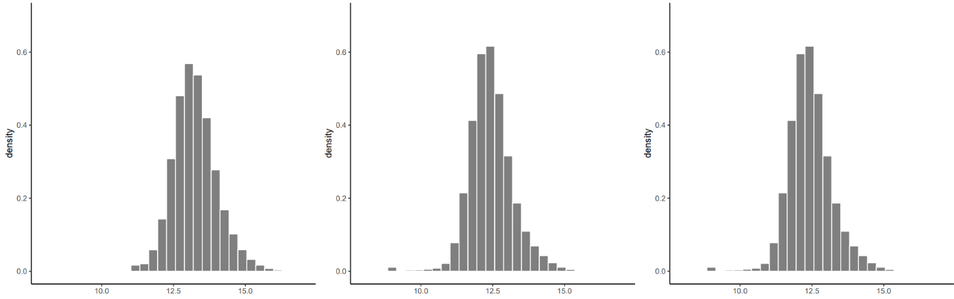
Figure 1.
Density of the Log-Shift transformation for per capita income for Colombia (left), Chile (center) and Perú (right). Source: Prepared by the authors.
The procedure consists in creating a new variable
Under this model, the vectors
According to [16], for those FGT indicators that can be defined as a function of
In this expression, the expected value of the response variable for out-of-sample elements within the domain
Since
To avoid the bias induced by ignoring the sampling design in the model, the parameters of the above distribution may consistently be estimated by including the sampling weights (
Being
Moreover, it is estimated by the following expression:
The estimation equation for the FGT poverty indicator of order
It is essential to clarify that the ratio of the number of sample units to the number of people in the country is low in most countries. Therefore the Census-EB predictor will perform quite similarly to Pseudo-EBP. We consider a Monte Carlo simulation procedure to estimate poverty indicators since the expectation that defines the best predictor often cannot be calculated analytically. The steps of the algorithm are as follows:
• Fit the unit-level model based on the survey data
• Estimate the vector of means
• For each small area
• Calculate the indicator of interest:
Although ECLAC uses its own poverty and extreme poverty lines for each country, they remain comparable. This way, Monte Carlo’s estimate of the Census-EB of the FGT indicator
In the estimation algorithm previously described, the Monte Carlo estimate of the FGT indicator depends on the vector of the regression coefficients
where
5.Prediction on small areas and their corresponding MSE
Note the importance of standardizing the relevant variables by applying homogeneous definitions and categories in both data sources. In this way, possible biases induced by the different measurements in the covariates or errors in the prediction due to different variables with similar names are ruled out. To this end, standardized structures and a dictionary of variables are generated that describes the categories and other necessary specifications. For instance, the variable “years of study” in censuses is created using the criteria adopted for surveys in BADEHOG.
We apply a parametric Bootstrap method to estimate the ECM of the Census-EB predictor. The unit-level models fitted to the survey data are replicated using census microdata. The algorithm considered describes a slight modification to the one published in (16) and has the following steps:
• Fit the nested error model to obtain the vector of estimators
• Generate Bootstrap effects for the small areas of interest
• Generate Bootstrap errors similarly but independently of
• Generate Bootstrap Pseudo-Census of the response variable for each country model:
• Where,
• Compute the FGT indicator of interest from the Bootstrap census
• For the same domains initially included in the household surveys of each country
is known as a pseudo sample.
• On the pseudo sample of households, adjust a mixed-effects model like the one used in step 1 of this algorithm and estimate Pseudo-EB Bootstrap predictors
Steps 2 through 7 are repeated
In this equation,
We exclude from the map any province, commune, and municipality with a coefficient of variation (
6.Model assumptions and benchmarking
Another stage of the procedure consists in benchmarking the results using the estimated FGT indicators from the survey at the national, national urban, national rural, and first administrative division levels. This guarantees consistency between the published figures as the aggregations of provinces, communes, and municipalities must be identical to those reported at different levels of disaggregation. This procedure also reduces the bias produced by a model miss-specification and improves the estimates’ quality in the provinces, communes, and municipalities.
In this step, we use the multivariate calibration of ratios described in [17]. The Monte Carlo simulation makes it possible to access the prediction vector for all the households in the pseudo-census. In addition, we have the poverty estimate from the survey. These quantities have the following ratio representation
For instance, using the survey poverty rates for national rural and national urban levels in each country, the benchmark algorithm would calibrate these ratios
After this stage, it is essential to carry out a strict validation and model assessment process to detect possible violations of the model assumptions. Tests used include the Kolmogorov-Smirnov, for normality (although it is also possible to use graphical diagnostics in the form of density kernels and quantile-quantile graphs) and White and Breusch-Pagan, for heteroskedasticity. Also, we use Cook’s distances as measures of the influence of the observations in the sample. The last stage uses geographic information for each country and shapes of interest (at the province, commune, and municipality level) to generate the maps.
7.Final remarks
This work aims to produce geographically disaggregated poverty indicators and produce maps to visualize the resulting estimates, helping policymakers to have a clear perspective on the incidence of the estimated indicator in different geographical domains, using different shades or colors to represent the magnitude of income and poverty indicators. The appendix presents a poverty map for 17 countries of Latin American, and poverty maps at the municipality-level for three countries: Chile, Perú and Colombia. All the poverty maps were adjusted using four cut-off points and a scale ranging from light green (lower poverty rate) to dark red (higher poverty rate) to illustrate the distribution of poverty by provinces, communes, or municipalities in the countries.
Figure 2 shows the SAE estimates for 17 countries in Latin America at the first administrative level, using similar cut-off points across countries to allow for regional comparison. Figures 3 to 5 refer to the EPB model at the second administrative level for Chile (Fig. 3), Perú (Fig. 4) and Colombia (Fig. 5). In this case, cut-off points are specific to each country, given the marked differences in their national poverty rates. Colombia has the highest poverty rates of the three countries under analysis. In Fig. 5 it can be observed that the poorest municipalities are located on the periphery of the country; specifically, in the Pacific region (Chocó, Cauca and Nariño), the Caribbean region (La Guajira, Magdalena, Bolívar, Sucre, Córdoba and Cesar), border departments (Norte de Santander and Arauca), and the Orinoquía and Amazon region (Vichada, Guainía, Vaupés, Amazonas and Caquetá).
In Peru, the highest poverty rates are in the border areas of the north and south of the country. Specifically, to the north, the highest incidence of poverty is concentrated in Loreto, Amazonas, the southern part of Cajamarca, and the western part of La Libertad. In the border area with Bolivia, another focus of poverty is observed in the regions of Puno and Cuzco.
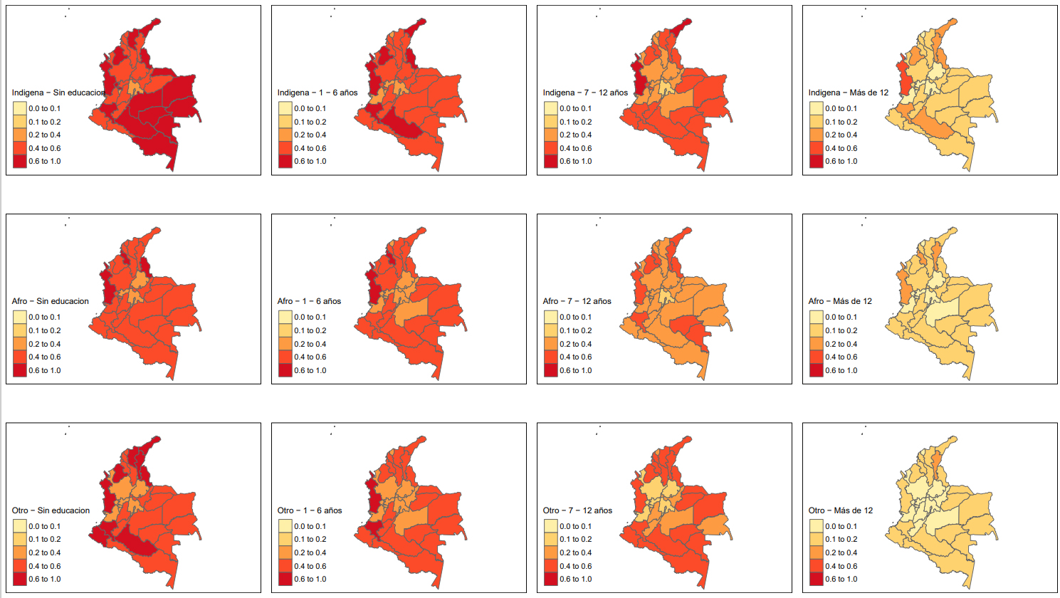
An important feature of poverty maps is to allow for disaggregation by geographical areas and individual or household characteristics relevant to poverty. Figure 6 shows how Colombia’s poverty affects people of indigenous origin and people with low educational attainment, disaggregated at the department level. This is particularly relevant in the context of the 2030 Agenda and its mandate to leave no one behind.
The use of SAE methodologies can lead to the production of highly disaggregated official statistics that describe the situation of different population groups and geographical areas as an essential input for public policies that aim to improve living conditions for all. Therefore, the methodologies described in this paper and their results are particularly relevant in the context of the 2030 Agenda and its mandate to leave no one behind.
In addition, visualizing this information on a map at disaggregated geographical levels emerges as an effective communication tool to facilitate the interpretation and analysis of spatial relationships. It can be a valuable input to establish priority areas of attention, implement the geographic targeting of public spending, and improve coverage of social programs, among others. In addition, contrasting the poverty maps with complementary geospatial information, such as the availability of roads or electricity, can lead to a better understanding of the interrelation between poverty and living conditions in general.
Acknowledgments
The responsibility for opinions expressed in this article rests solely with their authors and do not necesarily reflect the views of the United Nations. The authors thank the Director of ECLAC Statistics Division, Mr Rolando Ocampo, for continuous encouragement and express their sincere appreciation to the anonymous referee for valuable comments on a previous version of the paper.
References
[1] | ECLAC. Income poverty measurement: Updated methodology and results, ECLAC Methodologies. Santiago.: Economic Commission for Latin America and the Caribbean; (2018) . Report No.: 2. |
[2] | Foster J, Greer J, Thorbecke E. A class of decomposable poverty measures. Econometrica. (1984) ; 52: (3): 761–766. |
[3] | Feres J, Mancero M. Enfoques para la medición de la pobreza: breve revisión de la literatura. Serie Estudios Estadísticos y Prospectivos. (2001) ; (N |
[4] | United Nations. Work of the Statistical Commission pertaining to the 2030 Agenda for Sustainable Development. United National General Assembly; (2017) . Report No.: A/RES/71/313. |
[5] | Singh RANDHIR, Semwal DP, Rai A, Chhikara RS. Small area estimation of crop yield using remote sensing satellite data. International Journal of Remote Sensing. (2002) ; 23: (1): 49–56. |
[6] | Aybar Q, Wu L, Bautista R, Barja A. rgee: An R package for interacting with Google Earth Engine. Journal of Open Source Software. (2020) . |
[7] | United Nations. Achieving the Full Potential of Household Surveys in the SDG Era. Background document to the 50th session of the UN Statistical Commission. UN Statistical Commission; (2019) . |
[8] | Rao JNK, Molina I. Small area estimation Hoboken, NJ/: Wiley; (2015) . |
[9] | Deming WE, Stephan F. On a least squares adjustment of a sampled frequency table when the expected marginal totals are known. The Annals of Mathematical Statistics. (1940) ; 11: (4): 427–44. |
[10] | Goodman M. Comparison of small-area analysis techniques for estimating prevalence by race. Preventing Chronic Disease. (2010) ; 7: (2). |
[11] | Zhang X, Holt JB, Lu H, Wheaton AG, Ford ES, Greenlund KJ, et al. Multilevel regression and poststratification for small-area estimation of population health outcomes: A case study of chronic obstructive pulmonary disease prevalence using the behavioral risk factor surveillance system. American Journal of Epidemiology. (2014) ; 179: (8): 1025–1033. |
[12] | Gelman A, Hill J. Data analysis using regression and multilevel/hierarchical models: Cambridge university press; (2006) . |
[13] | Park DK, Gelman A, Bafumi J. Bayesian multilevel estimation with poststratification: State-level estimates from national polls. Political Analysis. (2004) ; 375–385. |
[14] | Guadarrama M, Molina I, y Rao JNK. Small area estimation of general parameters under complex sampling designs. Computational Statistics & Data Analysis. (2018) ; 121: : 20–40. |
[15] | Molina I, Rao JNK. Small area estimation of poverty indicators. Canadian Journal of Statistics. (2010) ; 38: : 369–385. |
[16] | Molina I. Desagregación de datos en encuestas de hogares: metodologías de estimación en áreas pequeñas. Santiago: Comisión Económica para América Latina y el Caribe; (2019) . |
[17] | Gutiérrez A, Zhang H, Rodríguez N. The performance of multivariate calibration on ratios, means and proportions. Colombian Journal of Statistics. (2016) ; 39: (2): 281–305. |
Appendices
Appendix
Figure 2.
SAE estimates of the extreme poverty rate in Latin American countries based on the Multilevel Regression with PostStratification approach. Source: Prepared by the authors.
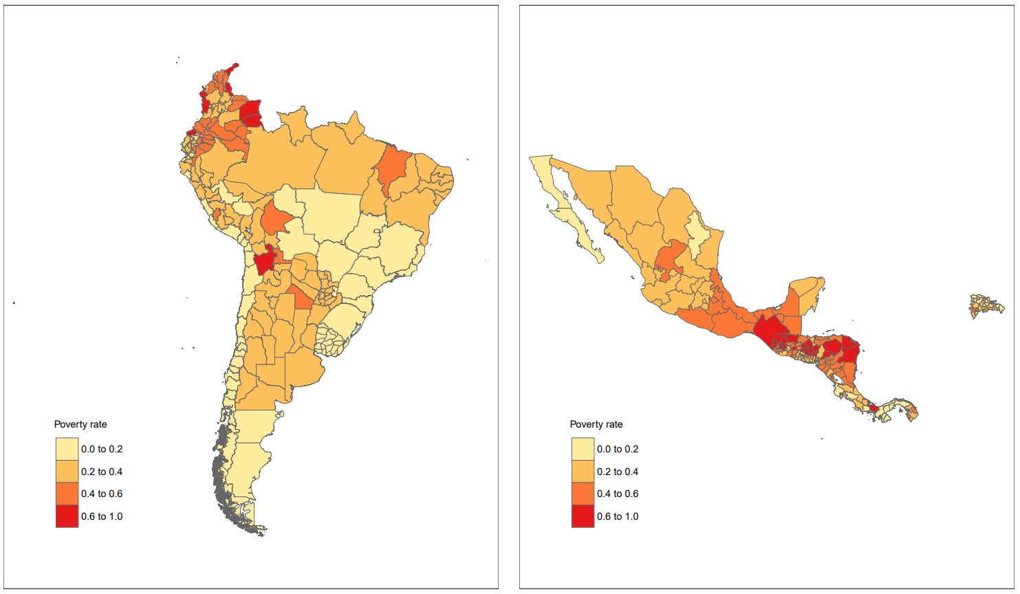
Figure 3.
SAE estimate of the poverty incidence rate in Chile for 2017 based on the EBP with sample weights approach. Source: Prepared by the authors.
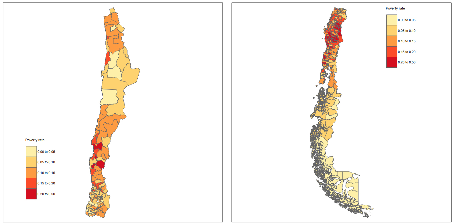
Figure 4.
SAE estimate of the poverty incidence rate in Perú for 2017 based on the EBP with sample weights approach. Source: Prepared by the authors.
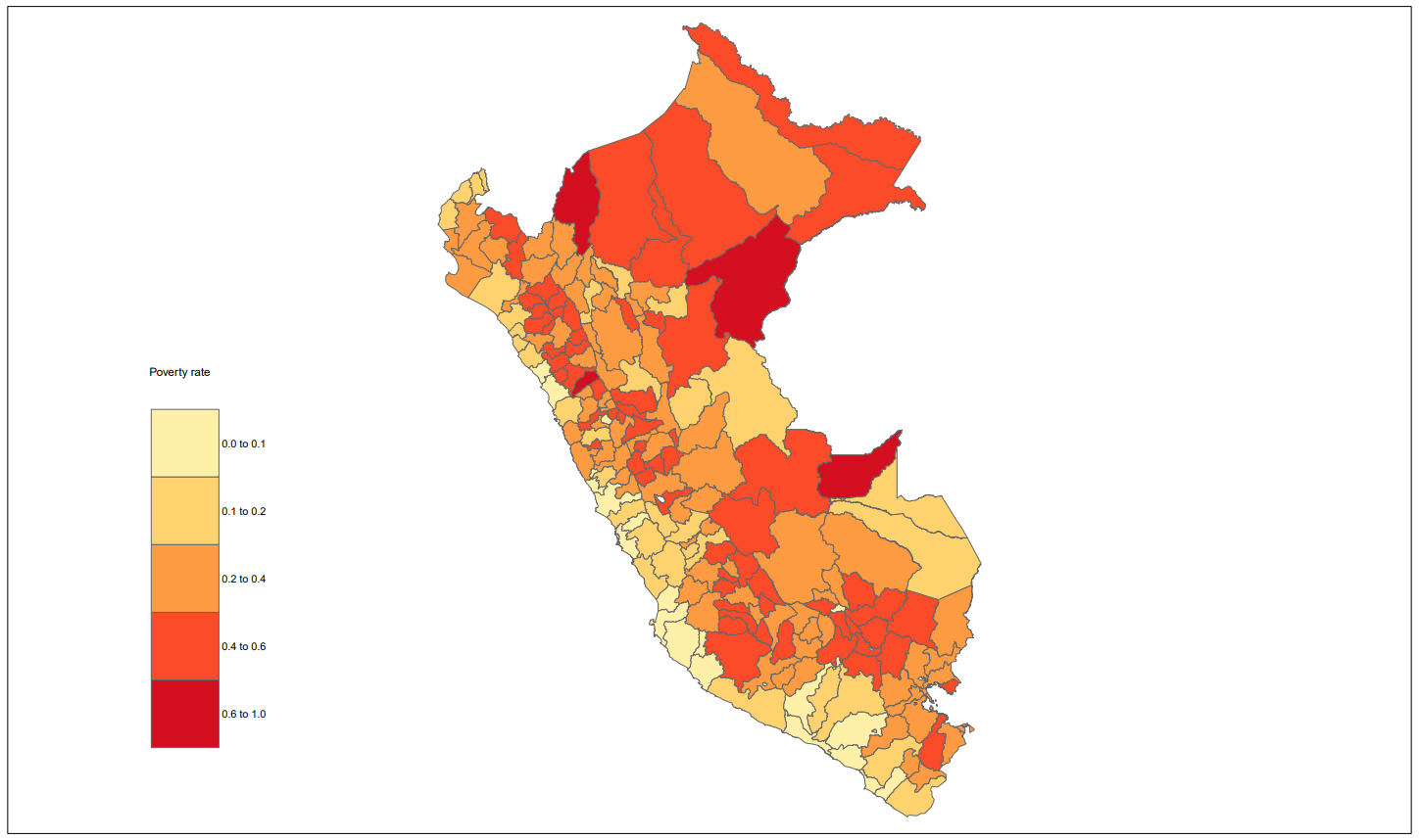
Figure 5.
SAE estimate of the poverty incidence rate in Colombia for 2018 based on the EBP with sample weights approach. Source: Prepared by the authors.
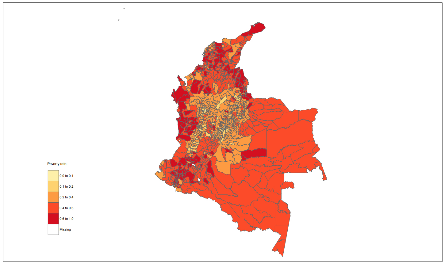
Figure 6.
SAE estimate of the poverty incidence rate in Colombia for the year 2018 disaggregated by ethnicity and level of education based on the Multilevel Regression with PostStratification approach. Source: Prepared by the authors.