The Eurostat business cycle clock and the pandemic: Some considerations

1.Introduction

Using dashboards of indicators is not new, in particular in relation to policy decision-making and monitoring. In the European Union there are numerous dashboards in use, for example the Euro Indicators dashboard, which gives an overview of the macroeconomic situation of a country or area in relation to economic and monetary conditions, which has been available since 2007 (see [1]). However, it can be hard to extract key signals from a dashboard containing numerous indicators, and users may prefer tools summarising main economic developments.

The economy is subject to cycles of expansion and contraction phases, and understanding in which phase we are, and if there are signs of a change of phase (for example, being close to a turning point), is one of the main issues tackled by econometric researchers. Fluctuations of the economy between periods of expansion and contraction have long been studied by business cycle analysts. Nevertheless, detecting turning points in the economy is not an easy task, and it becomes more difficult during exceptional times.

This task has become much more challenging during the recent pandemic. From one side, the statistical production has been confronted with new challenges to data collection and, when looking at the euro area, a new factor of complexity appeared: the lockdown measures taken at the national level to combat the pandemic have not been implemented in a synchronised way.

From another side, two main characteristics have made this period a special one requiring ad-hoc techniques: the crisis arose at very short notice and it started, first and foremost, as a health crisis and later became an economic crisis as well. The new challenge was how to treat unprecedented changes at the ends of the time series, which could be totally unrelated to the previous ones. Methods of smoothing or revising past values were not acceptable in such a situation: for instance, the very low level of industrial production at the start of the pandemic in the EU and the euro area (see [2, 3]) could not be estimated with previous values, and the series’ past evolution needed to be kept unchanged as if it was not impacted by the health crisis.

Eurostat has extensive experience in the construction and visualisation of turning point coincident indicators based on Markov Switching models. In this paper we would like to show the satisfactory results of the cyclical indicators at the base of the BCC tool during the pandemic, which showed a delay of only a few months in the detection of (provisional for the moment) turning points. Although this is not a statistical evaluation of the models underlying the indicators, as indeed they were adapted to maintain high performance in this turbulent time, we believe it can be of interest to assess how the BCC has tracked the pandemic.

The remainder of the paper is organised as follows: Section 2 will provide a short description of the BCC tool and its methodological context; Section 3 will describe some consequences of the pandemic on the statistical production of relevant variables for the BCC cyclical indicators; Section 4 will look at the impact of the pandemic on the values of input variables to the BCC cyclical indicators; Section 5 will describe how the models have been adapted to cope with the pandemic; Section 6 will display the results; Section 7 will shortly introduce a dashboard with non-macroeconomic dimensions as complementary information, and Section 8 will conclude.

2.The BCC tool: An overview

The Eurostat BCC is able to represent several aspects of cycles in a unique, visual context (see [4]). The idea at the base of the BCC is to look at the business, growth and acceleration cycles and representing the six possible states obtained by combining those three cycles in a unique image, a clock, which is at the same time familiar to the reader and conveys an intuition of cycles.

The BCC tool is based on three coincident probabilistic indicators for the business, growth and acceleration cycles, called the Business Coincident Cyclical Indicator (BCCI), the Growth Coincident Cyclical Indicator (GCCI) and the Acceleration Coincident Cyclical Indicator (ACCI). The values of these three indicators are combined to arrive at a single clock hand position.

The three cyclical indicators are computed by using Markov-Switching (MS) models which were introduced in the business cycle literature by Hamilton in 1989 (see [5]). Markov switching models were selected for the Eurostat BCC after a careful analysis of several alternatives. This choice has also been empirically validated in a comparison with other non-linear models (see [6]). MS models can be defined by associating cycle phases with different regimes. They are based on the concept of determining the probability of a variable of changing regime; changes in the regimes of the latent variable are then associated with economic regimes. Each cyclical indicator is a number between 0 and 1, representing the probability of being in a certain phase of the related cycle. Their analysis is combined with a threshold, which is usually set to be equal to 0.5. This is considered as the “natural” value for thresholds and it has been confirmed to perform well for our models too (you can find in [7] a discussion on alternative choices for thresholds; see also [8, 9, 10] for more information on the definition of MS models for the BCC tool).

We adopted a vector autoregressive Markov- Switching model for modelling jointly the BCCI and the GCCI, a pair of coincident indicators for the growth cycle and business cycle. Although the correct terminology should be MS-VAR GCCI and MS-VAR BCCI, for the sake of simplicity we will call the indicators GCCI and BCCI. The general (MS-VAR) model specification follows Krolzig’s notation (see [11]); models will be of the MSIH (K) – VAR (L) type, a Markov-Switching vector autoregressive model with (or without) intercept (I) and heteroscedasticity (H), where K is the number of regimes and L the number of lags of the autoregressive part (see [9] for more information on the models). In this multivariate approach the number of regimes chosen was fixed to four. This permits to better model the four phases of the business and growth cycles simultaneously and has been assessed as the best choice in terms of the models’ performance. The ACCI is the output of a univariate MS model returning the probability of a deceleration of the euro area growth rate cycle.

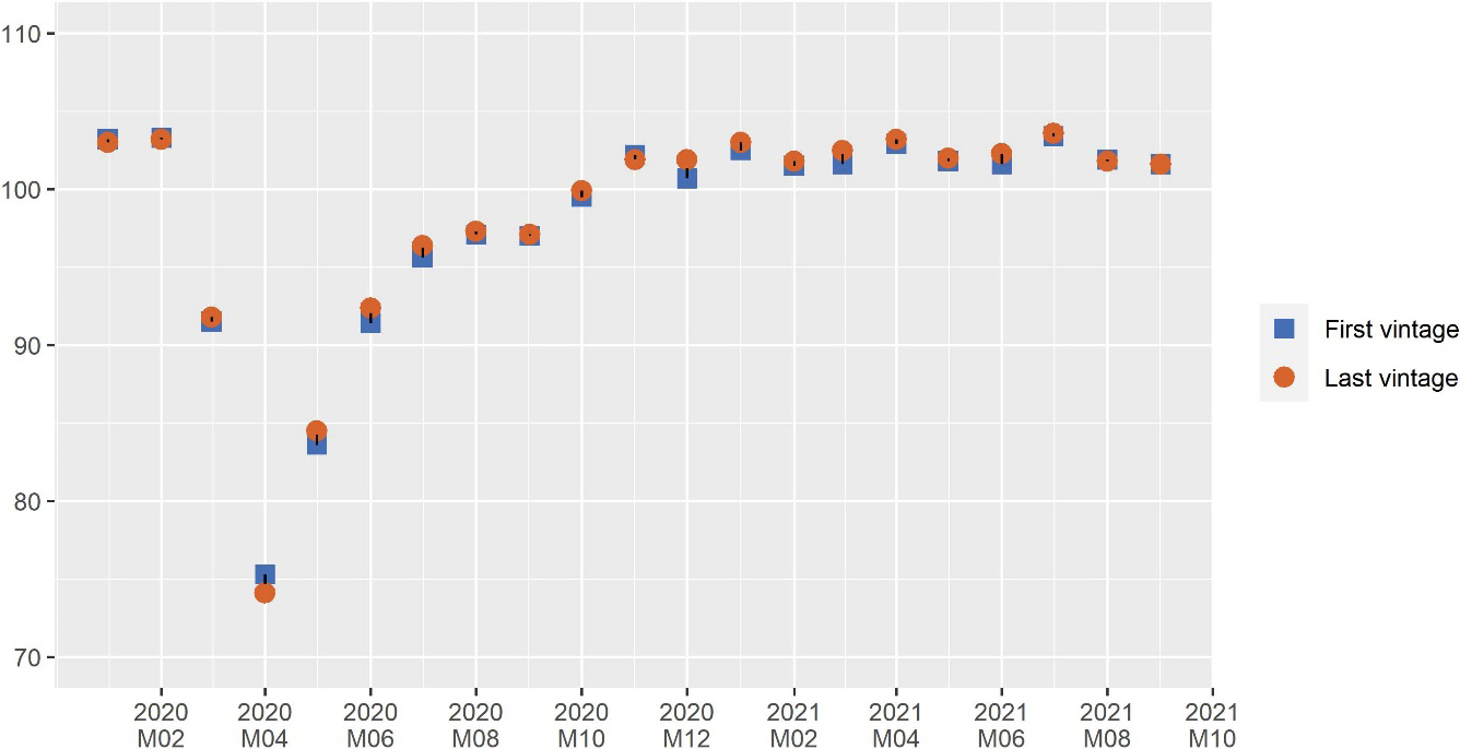
Figure 1.

Industrial production for the euro area – vintages (index 2015 = 100). Source: Eurostat.

The input variables to the multivariate MS model simultaneously computing the BCCI and the GCCI, which are composite indicators, are the industrial production index, the unemployment rate and two variables from the business and consumer surveys (run by the Directorate-General for Economic and Financial Affairs of the European Commission): the manufacturing employment expectations for the months ahead, and the financial situation of consumers over the last 12 months. The ACCI is computed by a univariate Markov Switching model based on the economic sentiment indicator (ESI), an indicator that is also part of the Business and Consumer Surveys. More information on the BCC tool and its methodological framework is available (see [8, 9, 10]); the online https://ec.europa.eu/eurostat/cache/bcc/bcc.htmltool. is available on the Eurostat website and it is updated monthly (see [4]).

The values of those three cyclical indicators are used to compute the position of the hand of the clock in the BCC tool, associating each clock sector to values of the three indicators.

3.How the pandemic affected statistical production of input variables to the BCC

The coronavirus disease (COVID-19) turned into a global pandemic by March 2020, with infections in more than 100 countries. The COVID-19 pandemic struck Europe suddenly and with great force. What started as a health crisis quickly translated into an economic crisis due to strict containment measures imposed by governments in most European Union (EU) Member States from mid-March 2020. The restrictions on mobility and public health measures, which were implemented in a bid to flatten the curve of infections and prevent healthcare systems from being overloaded, disrupted business activity across EU Member States. As a result, the European economy entered a sudden recession in the first half of 2020 with the deepest contraction in output recorded since World War II.

Enterprises reacted to the pandemic by temporarily closing, reducing production or even changing their economic activity. Closed enterprises did not send any data to statistical authorities, and the collection of administrative data was sometimes delayed (as governments eased reporting deadlines). As a result, one of the statistical challenges was the estimation of missing data in this completely new situation, unrelated to the past evolution of the statistics.

Despite concerns at the beginning of the pandemic in 2020, statistical production has proven to be resilient to the effects of the pandemic. All official statistical indicators for European aggregates have been released on time during the pandemic. The impact of the pandemic on the production of statistical variables and indicators feeding the BCC was, however, manifold.

One of the impacts of COVID-19 on time series has been to break existing seasonal patterns and to open the question on how to treat outliers in the seasonal adjustment process. Although this concerned the end of the time series, modelling an outlier at the end of a time series requires additional observations to decide the nature of the outlier, which could correspond, for example, to a temporary effect or to a definitive change in the level of the time series. As Eurostat’s https://ec.europa.eu/eurostat/documents/10186/10693286/Time_series_treatment_guidance.pdf Guidance on time series treatment in the context of theCOVID-19 crisis. mentions, changing the outlier type can have an impact on the series revisions and, as a consequence, can influence turning point identification. The outlier may be reflected in the trend-cycle component or in the irregular component, depending on the final specification. As an alternative, the use of intervention models could be explored (see [12] for an example).

An indirect effect of this last point is that seasonally adjusted data, such as the industrial production index, could be subject to higher revisions than usual, due to the adaption of the seasonal models to the availability of new data. Fortunately, it seems that for the euro area industrial production index, raw data revisions did not change the trend pattern provided by the first estimates (see Fig. 1).

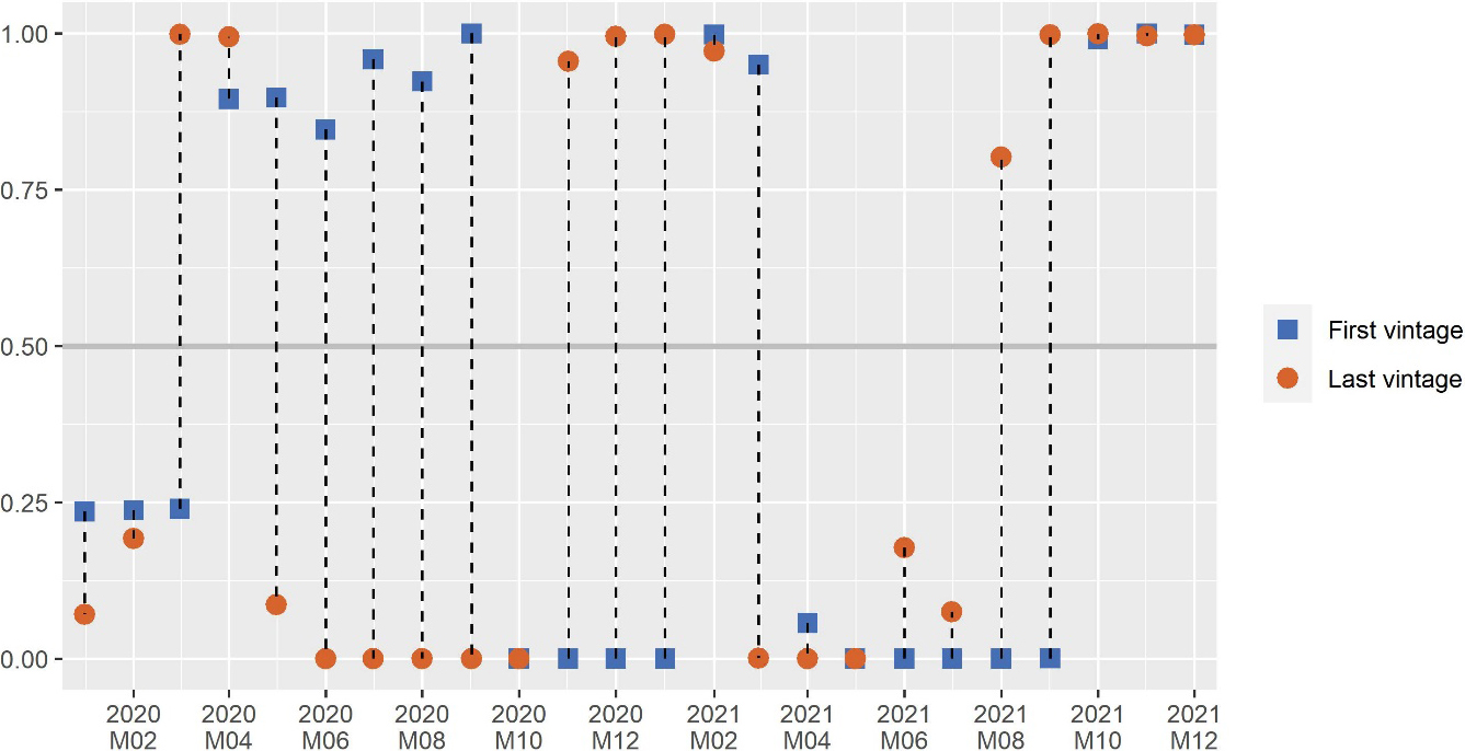
Figure 2.

Unemployment rate for the euro area – vintages (% of labour force). Source: Eurostat.

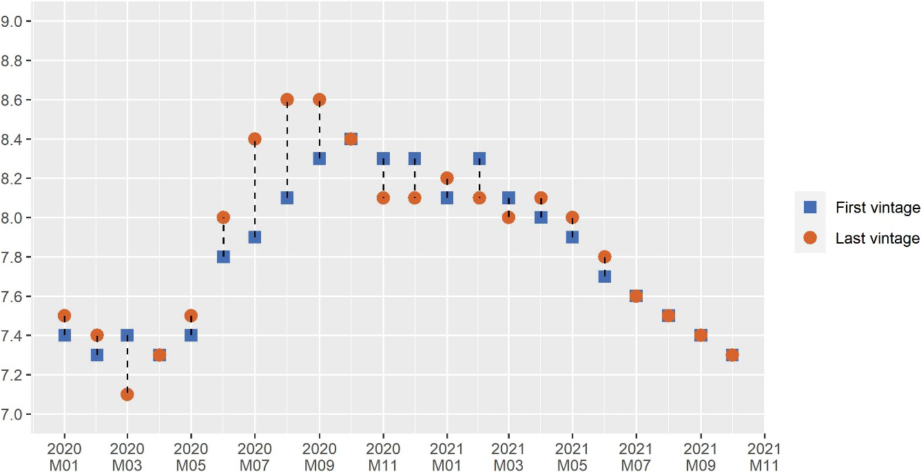
In the above figures, we compare the first estimated value, namely the first vintage, with the vintage available in January 2022, which we call the last vintage.

Another indicator used as an input in the BCC is the monthly unemployment rate. The monthly rates are benchmarked on quarterly results of the European Union Labour force survey (EU LFS), which is a continuous household survey carried out in all Member States in accordance with the harmonised definitions of the International Labour Organisation (ILO). The standard definition of unemployment counts as unemployed people without a job who have been actively seeking work in the last four weeks and are available to start work within the next two weeks.

The monthly data are interpolated/extrapolated by using national monthly survey data and/or national monthly series on registered unemployment which differs from the ILO definition. For most Member States the results from the LFS for a full quarter are available 75 days after the end of the reference period. The majority of the first estimates are usually provisional and subject to possible revisions.

The two concepts diverged more strongly during the pandemic, increasing the magnitude of revisions. This was due to the fact that a significant proportion of those who had registered in unemployment agencies were no longer actively looking for a job due to the pandemic. For instance, they may have been limited by the confinement measures or no longer available for work if they had to take care of their children during the lockdown. The turning points may also have shifted, depending on the goodness of fit between the quarterly LFS and the previously calculated administrative data pattern (see Fig. 2).

Looking at the Business and consumer surveys and the ESI indicator, although they are free from the above-mentioned impact of seasonal adjustment due to a specific adjustment procedure (DAINTIES) which does not revise past data (see [13]), some issues raised at the beginning of the pandemic had to be rapidly tackled. In March 2020, the containment measures launched to combat the spread of the virus were implemented in an asynchronous way across countries, so the timing of impacts on statistical data collections varied. Although in many countries the vast majority of survey responses were collected before such strict containment measures were enacted, accuracy and comparability across countries was potentially affected.

In April 2020 Italy, one of the biggest economies in the EU and of the most affected countries at the beginning of the pandemic, was not able to collect the necessary data for its surveys. The euro area and EU’s April values were then computed by a specific estimation, assuming that the changes compared to March were the same as in the aggregates excluding Italy. From the month of May 2020 no other impact on the collection of Business and Consumer Surveys data was observed. Nevertheless, the ESI indicator was subject to some minor revisions for the period up to the end of 2020 (see Fig. 3).

Figure 3.

Economic sentiment indicator for the euro area – vintages (long term average = 100). Source: DG ECFIN/Eurostat.

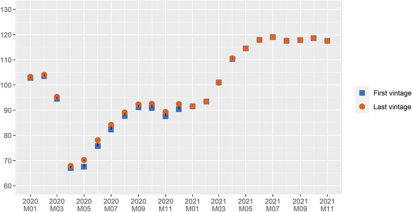
Figure 4.

Economic sentiment indicator for the euro area (long term average = 100). Source: DG ECFIN/Eurostat.

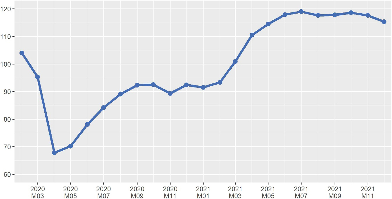
Figure 5.

GDP for the euro area (rebased index, 2019Q4 = 100). Source: Eurostat.

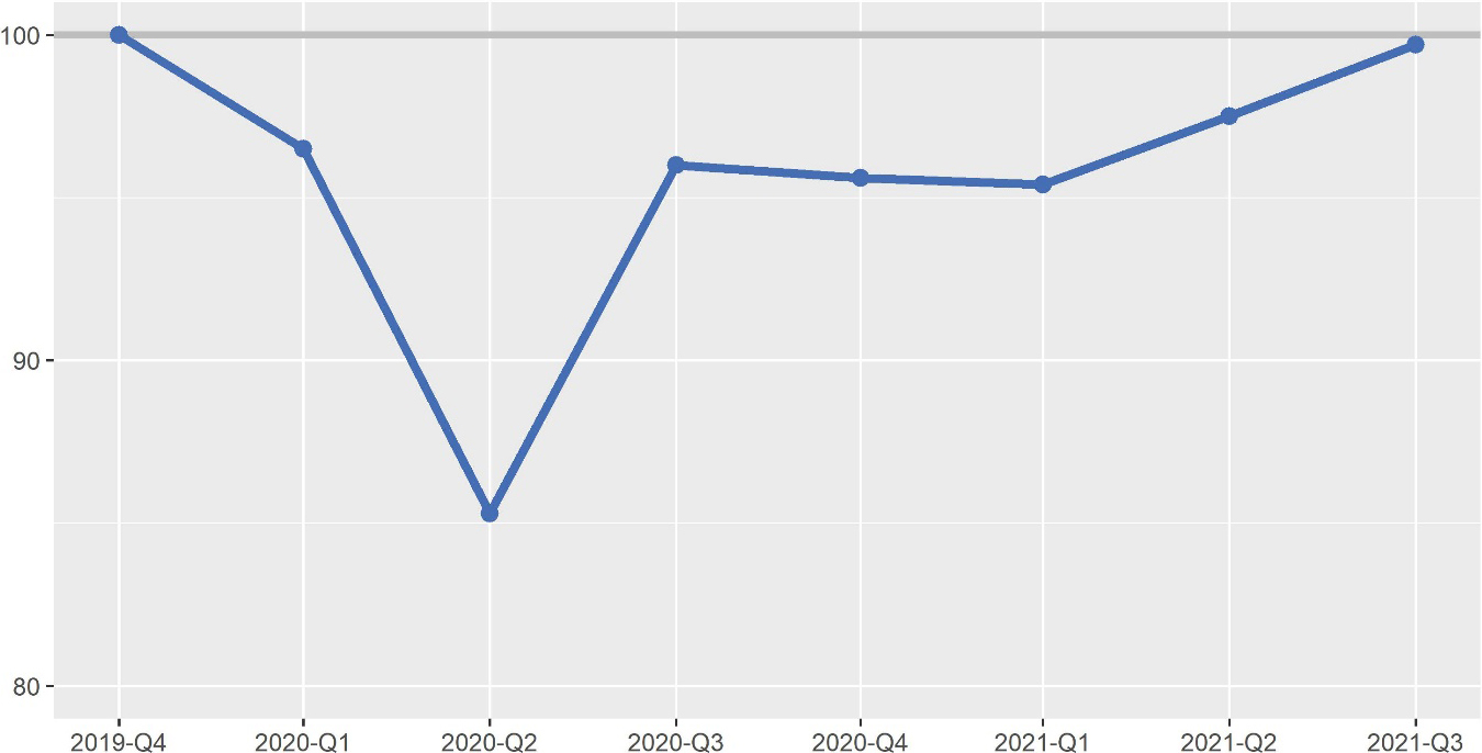
Figure 6.

Industrial production for the euro area (rebased index, 2020-02 = 100). Source: Eurostat.

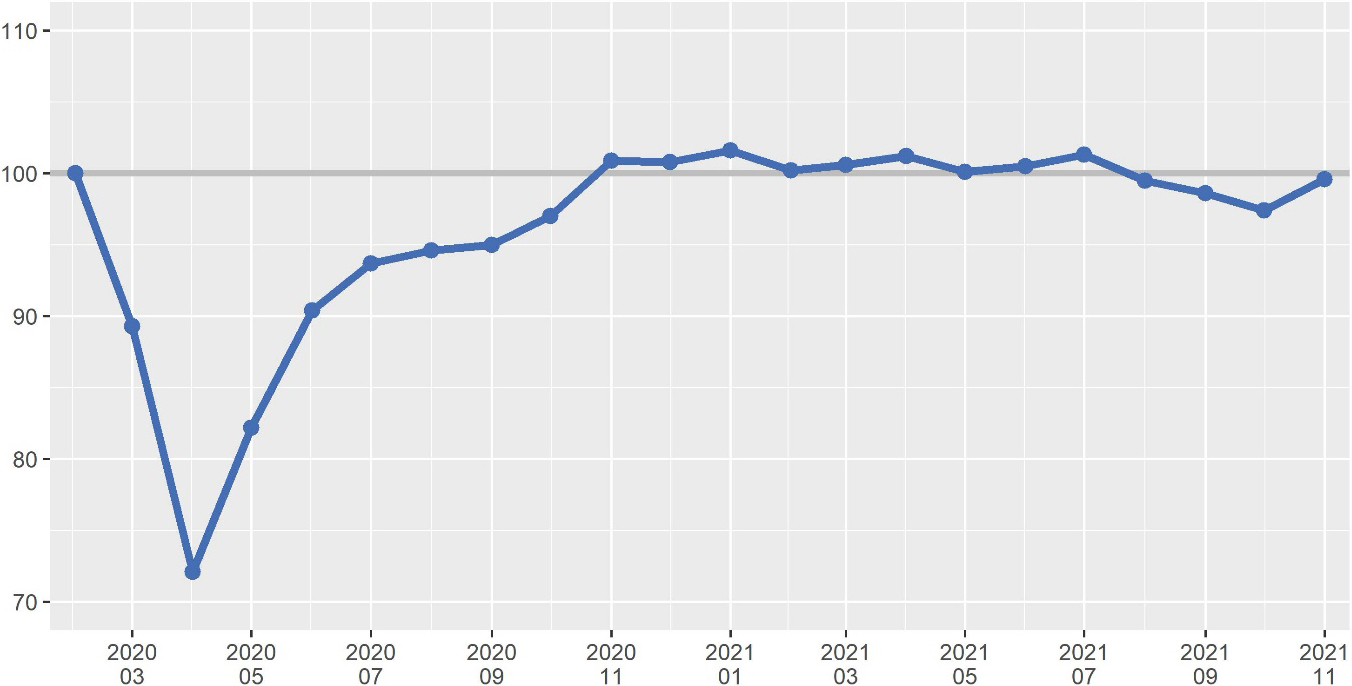
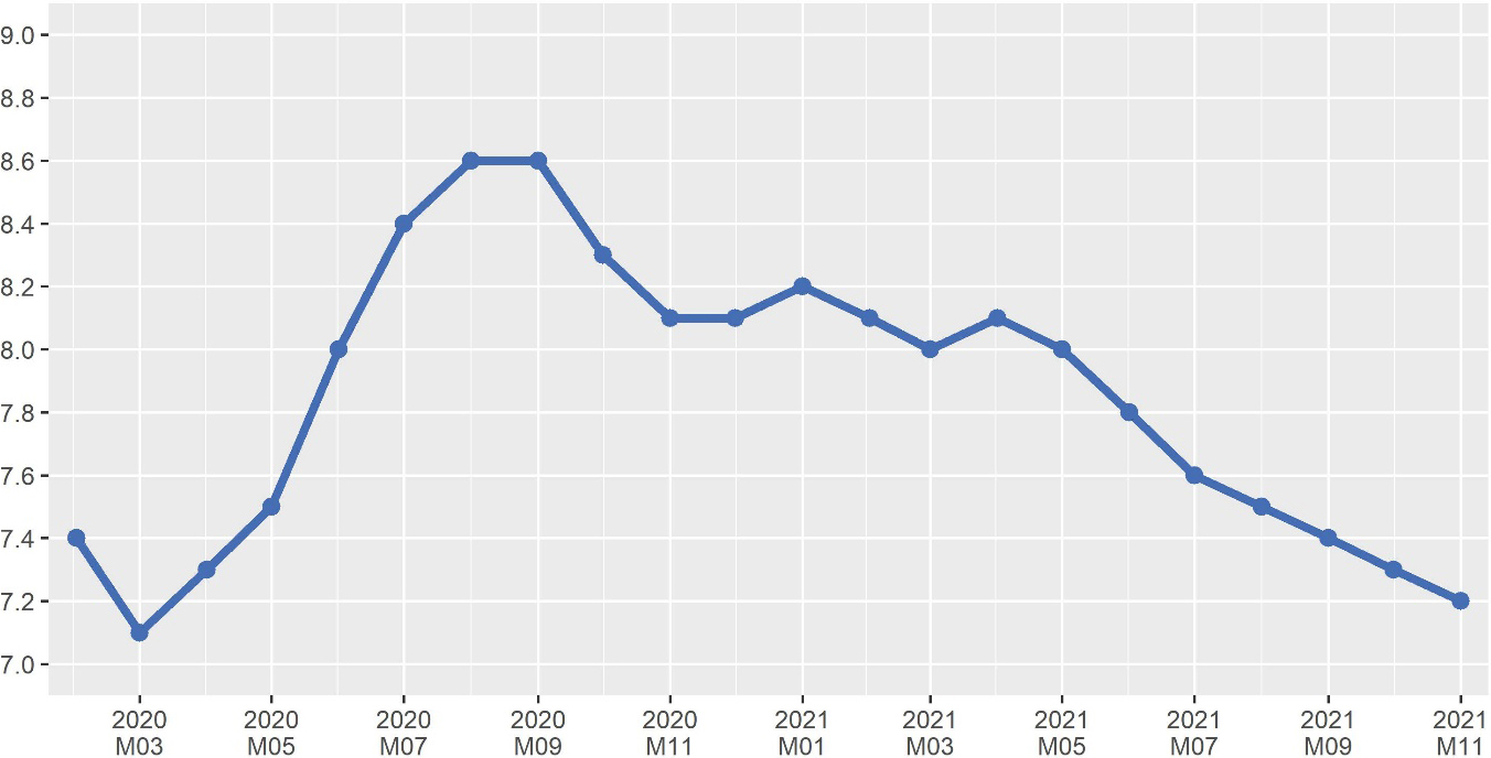
Figure 7.

Unemployment rate for the euro area (% of labour force). Source: Eurostat.

4.Impact of the pandemic on the values of input variables to the cyclical coincident indicators

As mentioned above, the outbreak of COVID-19 was followed by severe containment measures which caused a major drop in economic output. At the same time, the European Union rapidly adopted emergency support measures to facilitate recovery. It soon became evident that the crisis had an uneven impact in different economic sectors, with some hit hard by containment measures while others recovered rapidly after an initial shock.

In this section we will analyse the evolution during the pandemic of the values of the input variables to the coincident indicators: the economic sentiment indicator, the unemployment rate and the industrial production index.

The first glimpse into the negative impact of the pandemic containment measures on European economic output was provided by data from business and consumer surveys conducted by the European Commission (Directorate-General for Economic and Financial Affairs) in March 2020. The survey data showed slumping confidence among consumers and in all the business sectors. In March 2020, the economic sentiment indicator (ESI) plummeted by 8.7 points to 95.3 in the euro area and by 8.0 points to 95.9 points the EU. The March data still did not show the full impact of the pandemic on confidence among consumers and businesses as in many countries the majority of survey responses had been collected before containment measures were enacted.

The severe impact of containment measures was then reflected in the gross domestic product (GDP) data. In the first quarter of 2020, GDP contracted quarter-on-quarter by 3.5% in the euro area, and by 3.1% in the EU.

Afterwards, monthly data of short-term business statistics painted a starker picture for businesses. In March 2020, industrial production dived month-on-month by 11.0% in the euro area and 10.3% in the EU.

The collapse in economic output was overall deeper in the second quarter of 2020, reflecting the spread of the pandemic and the corresponding intensification of containment measures in April. In the second quarter of 2020, GDP fell quarter-on-quarter by 11.7% in the euro area and 11.3% in the EU. These were by far the sharpest declines observed since the time series started in 1995, significantly higher than the falls of around 3% recorded in the first quarter of 2009 during the financial crisis (see [14] for an analysis of the financial crisis impact).

Monthly data of short-term business statistics showed a further and even stronger decline in business activity in April 2020. Industrial production collapsed month-on-month by 19.3% in the euro area and 19.2% in the EU. Then in May 2020, a month marked by relaxing containment measures across countries, industrial output rebounded month-on-month by 14.0% in the euro area and 13.1% in the EU, and continued to expand by 9.3% in the euro area and 9.5% in the EU in June 2020.

Data from April 2020 also showed the severe impact of the pandemic on confidence among consumers and businesses. The ESI plummeted by 27.5 points to 67.8. This was the strongest monthly decline in the ESI on record, surpassing by far the fall in March. The ESI rebounded in May 2020, reaching 78.1 in June 2020.

Regarding the situation in European labour markets in the first half of 2020, job losses were unprecedented, though the decline was much more contained than the drop in economic activity. The relatively muted shock on labour markets was largely due to the successful implementation of ambitious policy measures in all Member States, such as short-time work schemes and other support policies to avoid mass lay-offs and large income losses, notably to the groups and sectors that were particularly affected (see [15] for a more detailed discussion).

In the euro area, the monthly unemployment rate rose from 7.4% in February 2020 to 8.0% in June, whereas in the EU, this rate increased from 6.6% in February 2020 to 7.3% in June. It is worth noting, however, that these estimates did not capture in full the unprecedented labour market situation triggered by the containment measures. In particular, they did not capture a sharp increase in the number of claims for unemployment benefits across the EU in March and April 2020.

An analysis of the impact of the pandemic on the labour market and on labour productivity is beyond the scope of this paper. However, it is worth mentioning that the difficult conditions of the pandemic were reflected in people’s labour status, which could change from being unemployed to being outside the labour force due to not being able to seek or accept work due to lockdown measures and health concerns. Moreover, the number of hours worked could decrease without a direct impact on the unemployment rate (see [16] for a more in-depth analysis). These shortcomings have generated interest in new indicators, such as labour market slack, which measures unmet needs for employment by considering the sum of unemployed persons (according to the ILO definition), underemployed part-time workers (those part-time workers who wish to work more), and persons either seeking work but not immediately available or available to work but not seeking it. The metric can be complemented by indicators on labour market flows showing the movements of individuals between employment, unemployment and economic inactivity. Those indicators are part of the recovery dashboard described in Section 8.

After an unprecedented contraction in the first half of the year, economic activity bounced back strongly in the third quarter of 2020 as containment measures were eased or lifted in Member States. GDP increased quarter-on-quarter by 12.6% in the euro area and 11.8% in the EU in the third quarter of 2020. However, economic output was still well below its pre-pandemic level of the fourth quarter of 2019. It took one further year before GDP got close to its pre-pandemic level, mainly due to the resurgence of more contagious variants of COVID-19 in the fourth quarter of 2020, aggravating the epidemiological situation and leading to renewed containment measures across the EU. Economic output was less severely impacted by subsequent renewed containment measures, showing economic resilience. In the euro area, GDP decreased quarter-on-quarter by 0.4% in the fourth quarter of 2020 and by 0.2% in the first quarter of 2021 (-0.2% and 0%, respectively, in the EU). GDP then increased quarter-on-quarter by 2.2% in the second and third quarters of 2021 (2.1% for both quarters in the EU).

Industrial production has, nevertheless, recovered much faster than the European economy as a whole. In November 2020, industrial output nearly reached pre-pandemic levels of February 2020, and then continued to oscillate around this level in 2021 as, in addition to containment measures at the beginning of 2021, the shortages of semiconductors and other materials started to weigh on manufacturers from the second part of 2021.

With regards to the labour market, increases in unemployment remained contained in the second half of 2020. Following a peak in August and September 2020 at 8.6% in the euro area and 7.7% in the EU, the unemployment rate started to fall as economic activity rebounded and the impact of renewed containment measures remained rather limited on employment. By September 2021, the unemployment rate decreased to 7.4% in the euro area, reaching its pre-pandemic February 2020 level, while in the EU, the unemployment rate was 6.7%, up by only 0.1 percentage points compared with its pre-pandemic level.

Economic confidence started to improve in the summer of 2020 but became more volatile in the winter. Economic confidence was eventually boosted significantly in spring 2021 by the breakthrough development of vaccines and the establishment of vaccination campaigns in all Member States. In April 2021, the economic sentiment indicator exceeded its pre-pandemic level for the first time since the outbreak of the pandemic in Europe. It continued to improve through summer 2021, reaching 118.6 in the euro area and 117.6 in the EU in October 2021, up from 104.0 and 103.9, respectively, in February 2020.

5.Adapting the BCC methodology to unprecedented shocks

Models aiming at turning point detection should be able to rapidly react to the latest available information. During the pandemic, this characteristic became both more important and extremely challenging.

The multivariate model used before the pandemic to compute the BCCI and the GCCI, estimated at the end of month m produced filtered probabilities until month m-2 while more recent information, for example on the surveys, was discarded. This was justified by a focus on the release dates of the industrial production index.

During the pandemic, we decided to improve the timeliness of the model. Two alternatives were considered. One possibility was to first build separate models for the most up-to-date variables, then estimating updated filtered probability of such variables. Those filtered probabilities could then be used as inputs in the standard model to compute the cyclical indicators. This approach was not employed in the end, both due to its complexity and because it requires the use of only two regimes in the factor model, while using four regimes has proven to be a better choice to model phases of the business and growth cycles in our experience (please refer to [17, 18] for a detailed description of the changes described in this section).

The second ultimately employed approach, was to align the model to the releases of the unemployment rate, which is the most up to date “hard” variable present in the model. In such a way, the modified model returns filtered probabilities until the month m-1 for the month m. This permits making the best possible use of up-to-date information. We consider in the estimation the last available values for the survey data, which are usually released at the end of the month until the current month m, together with the unemployment rate, which is released around the end of month m until month m-1. To make a concrete example at the end of March, the March values of the survey data will be released, while the last available period for the unemployment rate will be February.

As described earlier, the COVID-19 pandemic caused discontinuities in the economic indicators used as endogenous variables in the coincident indicators contributing to the BCC. For example, the industrial production index (IPI) experienced a very large decrease in April 2020 followed by a similarly large rebound in August 2020.

This resulted in convergence issues for the estimation of the parameters of the adopted models. The Expectation Maximization (EM) algorithm used to estimate the multivariate Markov-Switching model for the GCCI and BCCI indicators did not converge, and the same held for the procedure used to estimate the model underpinning the ACCI (see [17, 19, 20] for more information on the EM algorithm and the treatment of non-convergence).

Concerning the BCCI and the GCCI, finding a new model specification under pandemic conditions was challenging due to the non-economic nature of the shock and the unpredictability of the spread of the pandemic and its consequences at a macroeconomic level. It was therefore decided to trim the IPI in order to reduce its volatility. In such a way, without any model re-specification, the EM algorithm converged and the two indicators were able to better track the economic evolution during the pandemic. Filtered probabilities with and without this pre-processing, for the period before the non-convergence issue, were analysed and compared, showing more stable and reliable signals when using trimmed input data (see [18] for more details). This temporary solution could be revised in future, when better information is available, for example by adding one or more intervention variables to the MS-VAR model. A first comparative analysis of those two alternatives gave very similar results; as a consequence, the simpler solution was favoured.

Figure 8.

Growth cycle coincidence indicator for the euro area – vintages (probabilities for slowdown). Source: own calculations.

Looking at the ACCI, the MS model is a univariate MS model, based on a transformation of the economic sentiment indicator (ESI) aiming at eliminating noise and putting in evidence the cyclical movements of this acceleration cycle (1-month change of the 6-month difference). During the pandemic, the procedure used to estimate the model underpinning the ACCI did not converge either due to the sharp decline observed in the ESI starting in April 2020, which resulted in a drop of more than 10 standard deviations in the transformed ESI. It was then decided to alter the model to account for heteroscedasticity That results in a model of the form: MSIH(3)-AR(0). Furthermore, the definition of the ACCI was changed to the sum of the filtered probabilities of the first two regimes, instead of the first regime alone, improving the match with previously released values.

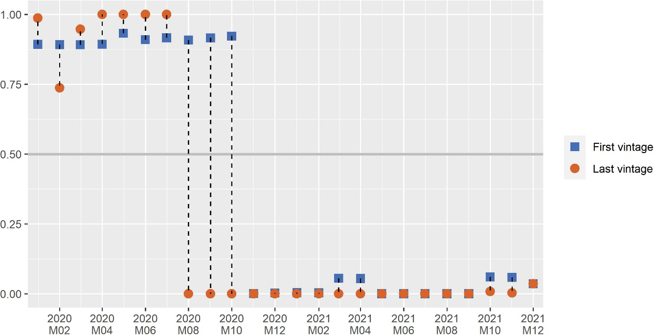
Figure 9.

Business cycle coincidence indicator for the euro area – vintages (probabilities for recession). Source: own calculations.

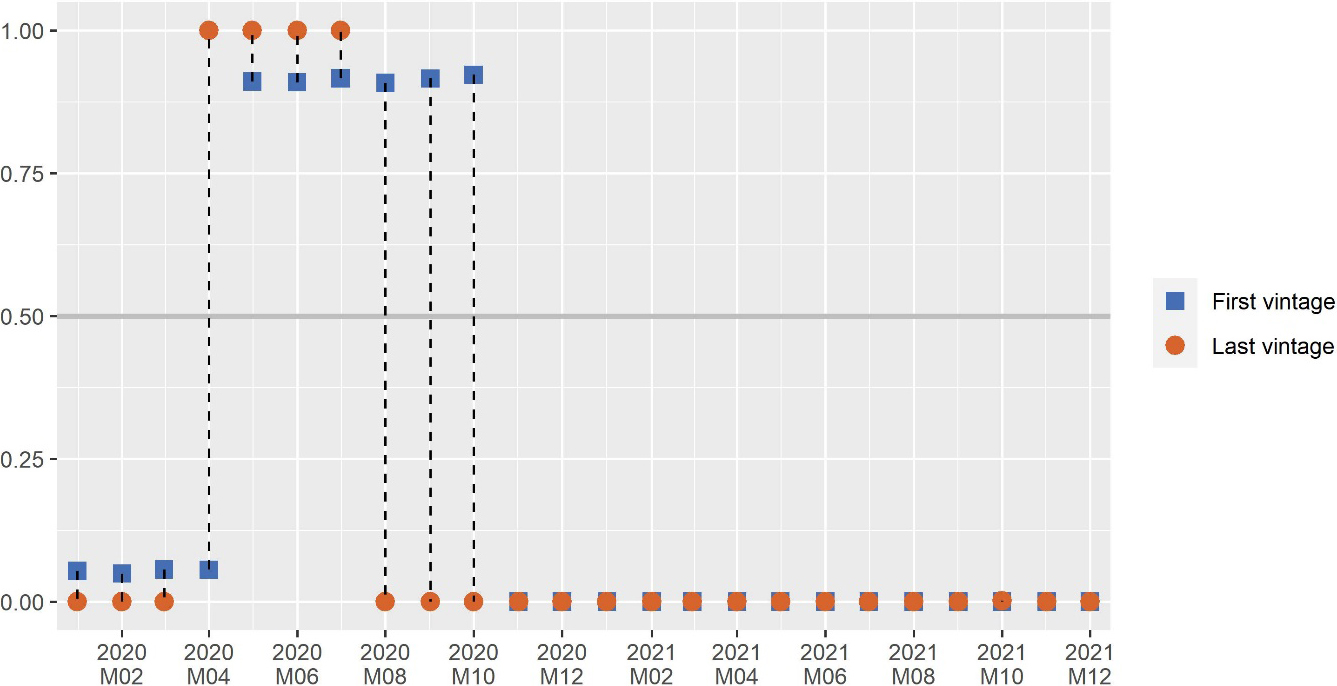
Figure 10.

Acceleration cycle coincidence indicator for the euro area – vintages (probabilities for deceleration). Source: own calculations.

Those adaptations to the models provided satisfactory results in terms of tracking economic developments even during the pandemic, as shown in the following section.

Finally, we also improved the assessment of the models’ results. The set of measures used in the assessment consisted of the Concordance Index (see [9] for a definition and [21]) and Brier score (introduced by Brier in 1950, see [22] for more details). In order to enlarge the set of performance measures, we looked at the domains of classifiers algorithms and machine learning, and adopted three new measures: precision, recall and F1 (the harmonic mean of precision and recall). Those measures give better insight into the performance of cyclical indicators, in particular because they better monitor imbalanced panels, which is the case of the business cycle because recession phases are rarer with respect to deceleration and slowdown phases in the acceleration and growth cycle respectively.

6.Indications of the cyclical coincidence indicators and their revisions

This section looks at the indications of the coincidence indicators as released in the BCC and their revisions. We compare the first computed value, namely the first vintage, with the vintage available in January 2022, which we call the last vintage. It is important to note that differences between the first and the last vintages could be partially due to changes in the methodology described earlier, so that this comparison is not an assessment of the underlying model, but an investigation of the stability of the values computed for the cyclical coincident indicators and the capacity of adapting the tool to the extraordinary circumstances of the pandemic.

Figure 8 presents the estimates of the growth cycle coincident indicator for the euro area. The figure shows the first and the last vintage of slowdown probabilities for each reference month. The first vintage indicates slowdown probabilities above 0.5 until October 2020, while the last vintage indicates slowdown probabilities above 0.5 only until July 2020, signalling an expansionary phase for the euro area three months earlier compared to the first estimates.

Figure 9 presents the estimates of the business cycle coincident indicator for the euro area. The figure shows the first and the last vintages of recession probabilities for each reference month. It can be noted that the first vintage shows recession probabilities above 0.5 from May 2020, while the last vintage shows recession probabilities above 0.5 from April 2020, indicating the presence of recessionary signals for the euro area one month earlier compared to the first vintage. The first vintage shows recession probabilities above 0.5 until October 2020, while the last vintage shows recession probabilities above 0.5 only until July 2020, indicating the absence of recessionary signals for the euro area three months earlier compared to the first estimates.

Figure 10 presents the vintages of the acceleration cycle coincident indicator for the euro area. The acceleration cycle is characterised by the highest number of fluctuations and a high degree of volatility. As a result, it is the cycle most impacted by the uncertain economic situation.

Summing up, the difference in the first signalling of the BCC tool of a euro area recession was delayed by one quarter with respect to the most recent signals; considering the exceptional circumstances in which the models had to be adapted, we believe this is a quite satisfactory result.

The above results for the business and growth coincident indicators are confirmed by our own dating exercise available until the third quarter of 2021. The acceleration cycle is characterised by the highest number of fluctuations. According to the dating exercise, a business cycle peak happened in 2019 Q4 and troughs of the euro area’s acceleration, growth and business cycles occurred in 2020 Q2. A deceleration episode occurred between 2020 Q3 and 2021 Q1. These results are still provisional.

The CEPR-EABCN Euro Area Business Cycle Dating Committee determined that the euro area COVID-19 recession started after the last peak in 2019 Q4 and reached its trough in 2020 Q2 (see [23]).

Figure 11.

Business Cycle Clock’s indications for the euro area. Source: Eurostat.

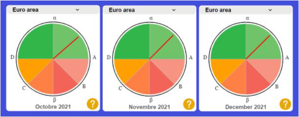
7.Recent indications of the clock

According to the indications of the business cycle clock for the fourth quarter of 2021 (see Fig. 11), the euro area economy remained in a ‘stable expansionary’ phase, although with decelerating growth. The hand of the clock has been stable between α (the peak of the acceleration cycle) and A (the peak of the growth cycle).

This means that the euro area persisted in its expansion after exiting the pandemic crisis. The deceleration of growth, signalled by the acceleration cycle coincident indicator, should not be necessarily interpreted as a negative signal for the future developments of the economy. The current signals provide a positive outlook. The clock indicates that the risk of another slowdown or recession (at this stage) is very low.

8.Looking forward: How to track the recovery?

In this section we would like to shortly introduce another available Eurostat dashboard which does not only focus on the macroeconomic dimension, but also includes social, environmental and health statistical variables which can be useful to track the recovery. The example of https://ec.europa.eu/eurostat/cache/recovery-dashboardthe European statistical recover dashboard. developed by Eurostat in December 2020 is an interesting presentational example, though it is presented as a dashboard of several indicators and does not extract a composite signal as the BCC does.

The recovery dashboard currently contains twenty-eight monthly and quarterly indicators from a number of statistical areas which are relevant for tracking the recovery across countries and time. The recovery dashboard was developed in cooperation with the statistical authorities in the Member States. It is updated every month with the latest available data and includes a Eurostat commentary for an analysis of the indicators. It also includes a number of innovative indicators such as excess mortality, number of commercial flights by reporting country, labour market slack together with flows showing the movements of individuals between employment, unemployment and economic inactivity, an air quality indicator and an indicator of greenhouse gases emissions.

The recovery dashboard is published as a visualization tool with user-friendly functionalities including easy data navigation, access to source data, and short indicator descriptions, among others.

9.Conclusions

Understanding large sets of macroeconomic indicators is not always straightforward; the Eurostat business cycle clock is a tool based on a robust methodology, giving synthetic signals on the state of the economy. It also enables deeper analysis of all phases of the economic cycles due to a joint analysis based on acceleration, growth and business cycles.

The pandemic arose at very short notice and it started as a health crisis to become then an economic one. We have leaved a period of highly uncertainty, with a sequence of asynchronous lock down measures across countries.

In this paper, we looked at the effect of the pandemic on the statistical variables feeding the tool and on the signals given by the tool. We have found that, in spite of challenging conditions to data collection, statistical production at European level has proven to be resilient to the effects of the pandemic. Moreover, the impact on labour markets, and in particular on the unemployment rate, was mitigated thanks to the successful implementation of ambitious policy measures in all Member States of the European Union.

However, a relevant effect of the pandemic was the high volatility of the variables feeding the BCC. We have discussed how high volatility caused non-convergence issues in estimating the parameters of the Markov-Switching models at the base of the BCC tool. We adapted the model for the ACCI, while we did not change the MS-VAR model for the BCCI and GCCI, because trimming the industrial production index was indeed enough to re-establish convergence.

Although the paper does not present a statistical evaluation of the models underlying the cyclical indicators, we consider the results satisfactory, showing only a few months of delay in identifying a change of phase of the business and growth cycles.

Finally, we looked at signs of recovery; after an unprecedented contraction in the first half of the year, economic activity bounced back strongly in the third quarter of 2020, with industrial production recovering much faster than the European economy as a whole. This has been confirmed by the recent signals of the BCC tool. According to the indications of the BCC, the euro area exited a recessionary phase in August 2020. In the fourth quarter of 2021, the euro area economy remained in a ‘stable expansionary’ phase, although with decelerating growth and the clock indicates that the risk of another slowdown or recession is very low at this stage in 2022.

References

[1] | Eurostat [Internet]. Euro indicators – Overview. Available from: https://ec.europa.eu/eurostat/web/euro-indicators. |
[2] | Eurostat [Internet]. News release of 13 May 2020 for industrial production. Available from: https://ec.europa.eu/eurostat/documents/2995521/10294804/4-13052020-AP-EN.pdf/dfa765ad-4a32-8135-f98f-69e565347750. |
[3] | Eurostat [Internet]. News release of 12 June 2020 for industrial production. Available from: https://ec.europa.eu/eurostat/documents/2995521/10294900/4-12062020-AP-EN.pdf/93c51a4c-e401-a66d-3ab3-6ecd51a1651. |
[4] | Eurostat [Internet]. Business Cycle Clock. Available from https://ec.europa.eu/eurostat/cache/bcc/bcc.html. |
[5] | Hamilton JD. A new approach to the economic analysis of nonstationary time series and the business cycle. Econometrica. (1989) ; (57): 357–384. |
[6] | Billio M, Ferrara L, Guégan D, Mazzi GL. Evaluation of regime switching models for real-time business cycle analysis of the euro area. Journal of Forecasting. John Wiley & Sons. (2013) ; 32: (7): 577–586. doi: 10.1002/for.2260. |
[7] | Ferrara L, Mazzi GL. Parametric models for cyclical turning points indicators. In: Handbook on Cyclical Composite indicators, Eurostat and United Nations, eds; (2017) . pp. 327–356. |
[8] | Ruggeri Cannata R. The Eurostat Business Cycle Clock: A complete overview of the tool. Statistical Journal of the IAOS. 37: (1): 309–323. |
[9] | Anas J, Carati L, Billio M, Ferrara L, Mazzi GL. Composite cyclical indicators detecting turning points within the ABCD framework. In: Handbook on Cyclical Composite indicators, Eurostat and United Nations, eds; (2017) . pp. 357–398. |
[10] | Billio M, Ferrara L, Mazzi GL, Ruggeri-Cannata R. Probabilistic coincident indicators of the classical and growth cycles, Eurostat statistical working papers. |
[11] | Krolzig HM. Markov-switching vector autoregressions. Modelling, statistical inference and application to business cycle analysis. Berlin: Springer; (1997) . |
[12] | Foley P. Seasonal adjustment of Irish official statistics during the COVID-19 crisis. Statistical Journal of the IAOS. 37: : 57–66. |
[13] | European Commission, The joint harmonised EU programme of business and consumer surveys – User guide, October (2021) . |
[14] | Eurostat [Internet]. The economic crisis in the non-financial business economy – where was it most heavily felt? Available from: https://ec.europa.eu/eurostat/documents/3433488/5564936/KS-SF-10-021-EN.PDF. |
[15] | Council of the EU [Internet]. Joint employment report 2022, adopted by the Council on 14 March 2022. Available from: https://data.consilium.europa.eu/doc/document/ST-7252-2022-INIT/en/pdf. |
[16] | Eurostat [Internet]. Hours of work and absences form work – quarterly statistics. Available at https://ec.europa.eu/eurostat/statistics-explained/index.php?title=Hours_of_work_and_absences_from_work_-_quarterly_statistics#Impact_of_COVID-19_pandemic_and_potential_recovery. |
[17] | Mazzi GL, Billio M, Carati L, Vlachou H. Towards the improvement of Eurostat’s turning points coincident indicators, presented at the NTTS 2021. |
[18] | Anas J, Billio M, Carati L, Mazzi GL, Vlachou H. Pandemics and uncertainty in business cycle analysis, presented at the SIS Satellite event on “Measuring uncertainty in key official economic statistics”, 17 June (2021) . |
[19] | Hamilton JD. Analysis of time series subject to changes in regime. Journal of Econometrics. (1990) ; (45): 39–70. |
[20] | Krolzig HM. Markov-switching vector autoregressions. Modelling, statistical inference and application to business cycle analysis. Berlin: Springer; (1997) . |
[21] | Harding D, Pagan A. Dissecting the cycle: A methodological investigation. Journal of Monetary Economics. (2002) ; 49: (2): 365–381. |
[22] | Brier GW. Verification of forecasts expressed in terms of probability. Monthly Weather Review. (1950) ; 78: : 1–3. |
[23] | CEPR-EABCN Euro Area Business Cycle Dating Committee [Internet]. A sui generis recovery is following a sui generis recession, findings published on 9 November 2021. Available from: https://eabcn.org/sites/default/files/_eabcdc_findings_-_9_november_2021_0.pdf. |
Appendices
Technical annex
This annex is largely drafted from the references in the bibliography (in particular from [8, 17, 18]). It aims to give some more details of the methodology at the base of the BCC tool.
1. Markov Switching models and probabilistic coincident indicators
The general specification of the Markov-switching model we consider is one in which all the parameters of the autoregressive model are conditioned on the state of the latent Markov-chain (st):
where p is the order of the AR model, the non-observed process st is a first-order ergodic discrete state Markov chain governing the realization of the unobservable state-variable, and εt is a standardized white noise process. The common latent state-variable that governs the changes in regime of the intercept term, the autoregressive coefficients and the variance-covariance matrix follows a first-order Markov chain with M regimes and time-invariant transition probabilities.
2. Parameters’ estimation
In order to estimates the parameters of the models, we use the maximum likelihood method in connection with the Expectation Maximization (EM) algorithm. The EM algorithm is a non-linear iterative technique for maximizing the likelihood function in case of models with missing observations or models where the observed time series depends on some unobservable latent stochastic variables. As a by-product of the estimation procedure we obtain the so-called filtered probabilities, which measure the probability of the latent variable being in a given regime j at a date t on the base of information as available at time t.
Under the assumption of time-invariant transition probabilities, the Markov-chain process above is defined by the transition probabilities:
Transition probabilities measure the probability of either staying in the same regime or switching to another regime from time t-1 to time t. The definition of a first-order Markov chain implies that the probability of observing regime j at time t depends only on the regime prevailing at the previous period.
3. Defining coincident cyclical Indicators
MS models can give in output different probabilities, that is a number in the [0, 1] interval; focusing on filtered probabilities, different phases of economic cycles can be associated to different states of the latent Markov chain in real time, when the obtained values are associated with a threshold. When setting the thresholds to 0.5, being over or below 0.5 will indicate in which phase the related cycle is: recession or expansion for the business cycle, slowdown or recovery for the growth cycle, acceleration or deceleration for the acceleration cycle. The GCCI and the BCCI are two composite cyclical indicators simultaneously estimated in a vector autoregressive Markov-Switching model, with the correct names being MS-VAR GCCI and MS-VAR BCCI. The ACCI is based on a univariate MS model.
a) Assessing cyclical Indicators
In order to assess the performance of cyclical indicators, it is necessary to compare the signals obtained with a reference chronology, that is a sequence of turning points. We have developed such a sequence and we first adopted two measures to assess how the cyclical indicators do perform: the QPS and the Concordance Index (CI). The QPS is defined as follows:
where, CoincidentIndicatort is either the probabilistic coincident indicator of the classical or growth cycle; RCt is a binary variable that represents the reference dating chronology of either the classical or growth cycle, which is equal to 1 during a recession/slowdown, respectively, and 0 otherwise.
In addition to the QPS, we also use a second accuracy criterion, namely the Concordance Index (CI). The Concordance Index, originally proposed by Harding and Pagan, is defined as follows:
where RCt is the reference dating chronology described above and It is a binary variable that assumes value 1 if the coincident indicator of either cycle provides a recession/slowdown signal.
Recently, we enlarged the assessment by the following metrics, borrowed from the classifier literature, to separately consider positive and negative signals:
• Precision = the number of true positives divided by the number of all positive (i.e. recession/slowdown/deceleration) returned by the classifier. Perfect precision corresponds to no false positive signals.
• Recall = the number of true positives divided by the periods that should have been identified as positive (i.e. recession/slowdown/deceleration). Perfect recall corresponds to no false negative signals.
• F1 = harmonic mean of precision and recall. In the
initial application, precision and recall are evenly weighted; however, further different versions of F score can be considered assigning higher weight to precision or recall, depending on the appetite for false positive and false negative signals, respectively.
b) Current models’ specifications
For the ACCI, the MSI(3)-AR(0) model used before the pandemic was re-specified to a state-dependent heteroscedastic model of the form: MSIH(3)-AR(0). Furthermore, to match as closely as possible the previously values of the ACCI, the definition has been changed to the sum of the filtered probabilities of the first two regimes, instead of the first regime alone previously considered.
The model specification of the estimation of the MS-BCCI and the MS-GCCI has not been changed; the trimming of the industrial production index has been enough to guarantee the convergence of the EM algorithm. The current model is of the form MSIH(4)-VAR(0).