
Combining farm and household surveys with modelling approaches to improve post-harvest loss estimates and reduce data collection costs
Abstract
While there is growing awareness of the issue of food losses at the political level, official post-harvest loss data for informing policymaking and reporting on SDG Indicator 12.3.1. (a) Food Loss Index is scarce. Representative sample-based surveys are necessary to obtain information on on-farm losses at the country level, but due to the issue’s complexity, a loss module covering several key questions is needed. One main strategy proposed by the 50x2030 Initiative for optimizing data collection is sub-sampling for some of the survey modules. This paper examines whether modelling approaches can be combined with sub-sampling to improve harvest and post-harvest loss estimates and allow for further sample and cost reduction. The paper first presents the loss models generated on four selected surveys conducted in Malawi, Zimbabwe, and Nigeria, which were built using the Classification and Regression Tree (CART) method. The performance of each model is assessed for different sizes of sub-samples to improve the sample-based estimates, either by model-based estimates or by model-based imputation. The research concludes that the model-based estimates improve the loss estimates of the sub-samples due to post-stratification implied in the CART method, whereby they can constitute a cost-effective complement to sub-sampling strategies, while model-based imputations should only be used on a reduced number of missing observations. The models perform best when the survey invests in obtaining more detailed on-farm loss data and considers some key variables identified as relevant for on-farm loss models. Sub-sampling allows for investment in more detailed questionnaires and some considerations are derived for its design.
1.Introduction
As part of Sustainable Development Goal Indicator 12.3.1 and the corresponding Food Loss Index [1] sub-indicator, a major discussion arises as to how to measure and monitor food losses at the country-level, covering the food supply chain from production up to, but not including, retail. The State of Food and Agriculture Report [2], estimates that along these stages 14% of total global food production is lost every year. Although losses differ considerably between commodities and countries, the farm is considered one of the most critical loss points, with direct impacts on farmers’ incomes, food security and natural resources [2]. Generating survey data at the farm level is one way of producing reliable estimates of harvest and post-harvest losses (PHL), to orient decision-making and monitor progress towards reducing food losses. Nevertheless, on-farm loss measurement is complex, and farm and household surveys can face several challenges in assessing and estimating these, as outlined by Kitinoja et al. [3], Xue et al. [4], Delgado et al. [5, 6], and Johnson et al. [7]. The multiple factors causing food losses, the different timings, stages and activities at which losses may occur, the considerable differences in the scale and cause of losses between commodities, typologies of actors, agro-ecological factors and management practices make measuring farm losses extremely burdensome. Collecting information on losses in farm and household surveys often requires breaking down the farm operations and asking the producer to quantify the losses for each operation [8]. This can be time-consuming, especially given that these questions need to be asked for each of the farm’s activities and crops and, in certain cases, for each plot (for harvest losses for example). It will also add to the respondents’ burden if the loss module is integrated in a broader farm or household survey and may therefore undermine data quality. If, in order to get more reliable data, losses are assessed through physical measurements or other methods [5], in complement to or instead of farmer declarations, the interviewers’ burden will be even higher as these operations require more time and highly skilled enumerators. Due to these challenges, properly assessing on-farm losses can result in a relatively high burden on the farm or household surveys and the overall data collection effort.
As part of the activities included in the 50x2030 Initiative to Close the Agricultural Data Gap (hereafter, “50x2030 Initiative”) an optional questionnaire module for collecting data on harvest and post-harvest losses on the farm has been designed [9].11,22 Such module, which largely builds on the experience learned in the framework of the Global Strategy to Improve Agricultural and Rural Statistics [8], combines declarative and physical measurements and can be added and integrated to the other 50x2030 survey instruments,33 depending on a country’s needs and demand. The 50x2030 Initiative, whose primary aim is supporting 50 low and lower-middle-income countries to strengthen the national data systems in order to produce timely and high-quality agricultural data countries thus can be instrumental to scaling-up the collection of data on on-farm losses and for assessing methods that can improve the estimates of losses generated from farm and household surveys.
In order to integrate the optional module on PHL within the modular 50x2030 Initiative survey system and in parallel optimize fieldwork implementation and data collection costs, sub-sampling of certain variables and modules is recommended in the 50x2030 Initiative sampling guidelines [10].44 The assessment of losses can thereby concentrate on a relatively small sub-sample of farmers and the freed resources invested into a more precise assessment of losses, either by detailing declarations or by using other methods to improve the estimates, such as visual scales and physical measurements.
In this context, farm loss modelling can constitute an additional instrument to support the sub-sampling strategy. Specifically, the models will be assessed to see if they can improve the loss estimates obtained from the smaller sample, either by using model-based estimates from post-stratification or model-based imputation. For doing so, the loss model is built on the sub-sample using a set of explanatory variables collected in the survey. The potential determinants are standard indicators to characterize the farm and its production system and may include, among others, socio-economic characteristics such as age and level of education, harvesting methods and number of harvesting days post-harvest technology used, information on the type of storage facility used, storage duration, use of pest control products during storage, as well as information on weather and production conditions. This research will examine whether farmlevel post-harvest loss models built on the available set of variables present sufficient reliability for prediction purposes. Afterwards, it will be assessed whether modelling approaches can add to the results based on sub-sampling, for instance by improving the estimates and/or allowing a further reduction of the sub-sample [11]. Apart from the objective to reduce data collection costs, the models also help better identify the causal factors of losses (e.g. addressing labor shortages, or promoting certain types of storage facility).
This article starts by summarizing the results of the literature review on loss models used in combination with farm survey data. A general approach is then presented to estimate on-farm loss models, covering the estimation strategies, model structure and relevant explanatory factors. This methodology is then used on available datasets from farm loss surveys and household surveys in Zimbabwe, Malawi and Nigeria. The performance of the models is assessed and the gains obtained from using them to improve the loss estimates and reduce data collection costs are outlined.
2.Literature review on post-harvest loss models
2.1Scope of the literature review
A literature review was conducted to identify whether on-farm loss models built using data from onfarm or household surveys have been estimated, how robust they were and what estimation strategy and set of explanatory factors were used. The review covered 126 journal publications that mentioned food loss models or post-harvest loss models in any form, of which 62 publications applied food loss models at the farm or household level. The nature of the models used largely depended on the objective of the modelling exercise and ranged from identifying the factors causing on-farm losses, to estimating losses indirectly or assessing the impact of losses or loss reduction on socio-economic factors, at the micro and macrolevel. For the purpose of this research, those papers estimating regression models to identify the drivers of losses were chosen to be the most relevant, since they were built on farm survey data and provided guidance for suitable sets of explanatory variables and the overall model structure.
The review shows that loss models estimated using farm survey data identify a wide range of significant explanatory factors. Most of these studies collected cross-sectional on-farm loss data on single commodities and sub-national regions, with only a few covering a larger number of crops. Africa is the most represented region (more than 25 papers), followed by Asia (15 papers), while fewer studies were found for the rest of the world. Great contributions to this research topic come from Ethiopia and Nigeria, followed by Bangladesh, Kenya, India, Nepal, Uganda and Ghana. Several studies build on each other, for instance Kumar et al. [12] and Basavaraja et al. [13] represent one of the first applications of regression analysis to determine on-farm loss drivers and were cited by various articles. The large majority of screened papers were produced between 2015 and 2020 and cover mainly grains (21 papers), roots and tubers (12 papers), and fruits and vegetables (19 papers). Some of the studies also conducted surveys and regressions for off-farm stages, but these were not further examined for the purpose of this research. In what follows, the main conclusions in terms of the estimation approach, the data used, and the dependent and explanatory variables are outlined.
2.2General model approaches used for farm loss modelling and survey data
The most commonly found estimation approach is a multiple linear regression, using a set of explanatory variables in order to explain the dependent variable of on-farm losses. This approach was used for instance by Kumar et al. [12] and Basavaraja et al. [13] on grains, roots and tubers in India; Begum [14] and Khatun et al. [15] on rice, wheat and tomato in Bangladesh; Arun et al. [16] and Paneru et al. [17] on a variety of commodities in Nepal; Adisa et al. [18] on yam; Babalola et al. [19] on tomato in Nigeria; Tadesse et al. [20] on potato in Ethiopia; and Ambler et al. [21] on cereals in Malawi. Some authors opted to use a double and semilogarithmic multiple regression analysis, as Folayan [22] on maize in Ethiopia, Aidoo et al. [23] on tomato in Ghana, and Huang et al. [24] on grains in China. Ansah et al. [25] used a fractional logistic regression model because of the proportional nature of the dependent variable, which in this case is post-harvest management as a way of assessing the inverse of on-farm losses. Hossain et al. [26] suggested a Cobb-Douglas production model to estimate the coefficients of the factors influencing potato storage losses in Bangladesh. Shee et al. [27] and Garikai [28] used an ordered probit model, employing on-farm loss categories that organize loss percentages into four loss categories. These categories were built from loss percentage data collected in the respective study survey. Amentae et al. [29] and Falola et al. [30] used a tobit regression model, applying only a binary category of on-farm losses (low and high losses; experience and do not experience losses). Kikulwe et al. [31] made use of a tobit censored regression model to solve the limitation in the dataset of a significant number of producers who reported zero losses.
Most of the surveys collected on-farm loss data by declaration together with other socio-economic characteristics of the producer or household, agronomic indicators of production or post-harvest management, and climatic and weather factors. Therefore, the data for the regression models was overly obtained from the same survey. In general terms, the surveys conducted for the loss studies had a sample size of about 100 to 300 households, depending on the target population, regional coverage and available resources.
2.3Set of dependent and independent variables used for the farm loss modelling
Almost all surveys estimated total post-harvest losses aggregated for all post-harvest activities, while only some studies disaggregated losses by or concentrated on one specific activity. Storage losses were one of the more specific areas of study (Kimenju et al. [32] on maize; Falola et al. [30] on yam; Hossain et al. [26] on potato). Ambler et al. [21] conducted the regression model on aggregated post-harvest losses as well as disaggregated by post-harvest operation for maize, soya and groundnuts. The main differences are the choice of independent variables, which are more specific if the study focuses on a single post-harvest activity. Two studies, namely Kikulwe et al. [31] on banana in Uganda and Qu et al. [32] on grains in China, also included harvest losses in addition to post-harvest losses. The most frequently used dependent variable is loss quantity in kilograms, as applied by Aidoo et al. [23] and Aidu et al. [34] in Ghana on tomato, Tadesse et al. [20] on potato in Ethiopia, or Folayan [22] on maize in Nigeria. Four studies considered on-farm loss in kilograms per hectare, as a way to relate the loss quantity to the size of the farm, as Kumar et al. [12] and Basavaraja et al. [13] in India and Begum [14] or Khatun et al. [15] in Bangladesh. On the other hand, six studies used loss percentage as the dependent variable, relating loss quantities to the total quantity produced, as Mebratie et al. [35] and Amentae et al. [29] on Ethiopia or Paneru et al. [17] and Arun et al. [16] on Nepal. Each of these three approaches can have different implications in terms of the relevance of loss drivers. Loss quantities are likely to be positively related to production volume and factors influenced by the size of the farm. Loss percentages are more commonly used to identify structural losses usually caused by the type of production system, climate, and agronomic practices. Loss quantities per hectare could be interpreted similarly to loss percentages, although it does not take into account the differences in productivity that are counted in when using loss percentages. Kikulwe et al. [31] applied a regression analysis on the drivers of loss quantities and loss percentages, which provides the possibility of comparing the changes in the significance of explanatory factors between both types of dependent variables. On the other hand, three studies (Shee et al. [27]; Maziku [36]; Garikai [28]) used on-farm loss categories of minimum, low, medium and/or high losses. These were either reported directly as categorical variables by the producer or based on the loss percentages the producer declared. Some studies (e.g., Kwami et al. [37] and Falola et al. [30] on food losses in yam and plantain in Nigeria) need to be analyzed separately as they build the regression analysis on the adaptation or use of technologies that are directly linked to higher or lower losses.
Apart from the general mapping, special emphasis was put on systematizing the explanatory variables used in these studies and their overall significance, which can be accessed in detail in the report of the 50x2030 Initiative literature review [38]. The studies show certain similarities in terms of the set of variables chosen. These cover a set of variables that can be grouped according to the household’s socio-economic characteristics, production characteristics, post-harvest management and market relations, and agro-ecological and weather conditions. Most studies cover each of these groups with at least one variable. In general terms, the group of production characteristics and agro-ecological and weather factors seem to have the most significant relation to on-farm losses, followed by post-harvest management and market relations, while socio-economic characteristics have a less significant impact. Within the production characteristics, production or farm size, the experience in farming and access to extension services and training, as well as the time or days of harvesting were those most commonly used and which showed to be significant for losses. Within the group of agro-ecological and weather factors, weather conditions during harvesting (rainfall during harvesting, good weather conditions during harvesting), the agro-ecological zones and general weather conditions (annual mean temperature) showed to be significant, as well as general geographical indicators (district, altitude). In terms of the group of post-harvest characteristics, the type and use of storage facilities (cereals and pulses), and the distance or time to the nearest market are relevant indicators, while those variables relating to other post-harvest operations like packaging, threshing and transportation provided less significant results. In terms of socio-economic variables, education, age and sex were the most commonly used, but resulted in limited explanatory power for on-farm losses. Family size was another widely used variable and had mixed results but with a tendency towards being significant.
3.Modelling approach
3.1The CART method for post-stratification to specify and identify the loss model
There are different uses of generalized linear models. One common use is to establish the relationships of selected independent variables as determinants of losses, while another is to predict mean responses, where the inclusion of a wide variety of independent variables are used as determinants focusing on the prediction capabilities and statistical efficiency of loss estimates. While the literature review highlights mainly on-farm loss models to identify on-farm loss drivers, this research seeks on formulating on-farm loss models for prediction purposes. Therefore the above-mentioned results from the literature review provide a key orientation point for specifying the models but need further discussion to generate models for prediction purposes. In this paper, the objective is to test one possible way of specifying on-farm loss models for prediction purposes making use of a classification method derived from a Classification and Regression Tree (CART) post-stratification [39, 40]. It is expected that this modelling approach not only provides good and reliable on-farm loss estimates, moreover it simplifies the modeling procedure and helps to improve the efficiency of the mean estimate by a reduction of its standard error. These gains, in turn, can support data collection on relatively small sub-samples. Data collection costs could be optimized without considerably compromising data quality, resulting in a complementing strategy to be used to design national data collection of losses within national farm and household surveys.
As a first step, a better understanding of the available survey datasets is needed, especially on the overall availability of significant variables from the surveys to explain on-farm losses. Based on the insights obtained from the literature review multiple linear regression models were tested, choosing a set of independent variables related to harvest and post-harvest known to be relevant for losses. On the other hand, different dependent variables proposed in the literature were thereby assessed to revise whether to use quantity losses or percentage losses, total post-harvest losses or losses disaggregated by operation (harvest, cleaning, drying, storage, etc.) As a first conclusion, on-farm loss percentages seem to be a better suited dependent variable than quantity on-farm losses for the given survey datasets. Percentage losses seem to better indicate the structural problems causing losses, the efficiency of handling the grains, while the quantity of losses is to some extent driven by the production volume. Since the recorded percentage losses show a positive skewed distribution, the use of the natural log transformation of the percentage losses is suggested. A linear regression could be used to generate a model to predict mean percentage losses, but in that case, predictions from the model are in log scale and the reverse transformation results in a bias of the estimated mean losses. These could be corrected by including a function of the variance of the errors in the estimated mean losses. Nevertheless, the use of a Poisson regression model can be a better alternative to log-linear regression, because the link function of this model is the natural log of the response. Additionally, a Poisson regression handles outcomes that are true zeros, while a log regression does not consider zeros because of ln(0) is
As a second step, post-stratification is prepared with the main idea to improve the efficiency of the parameter estimates obtained from the sample survey and respective sub-samples. As stated by Smith [41], it can be a useful method to reduce variance and correct for possible bias, and in this case Classification and Regression Trees (CART) are used to generate the post-stratification. The output of the CART is a decision tree where each end node represents a stratum with a final prediction for the outcome variable, in this case on-farm losses. The algorithm selects the relevant independent variables and their respective cutting point where the difference of the mean response for the resulting groups are maximized. Thereby, part of the variance in the sample survey is explained by the mean differences between the resulting groups. In order to make use of post-stratification in the modelling approach, the results of the classification and regression tree are used to set the estimation model, where the classification variable is used as predictor and the mean prediction is used as the estimator of the mean on-farm loss. In what follows, the models are tested to determine whether they (i) are sufficiently well-specified to provide reliable estimates, and (ii) reduce the standard error as an assumed effect of the post-stratification procedure.
To test if the model is well suited, the linktest [42] is used to detect any specification error in the proposed models. This uses the linear predictor value
3.2Evaluate the gains of the modelling approach for sample size reduction
The main idea of this research is to make use of the improvements in the mean estimate obtained from post-stratification in order to reduce on-farm loss data collection to a sub-sample. The models will be assessed on the basis of their capacity to produce estimates, which should not deviate considerably from the estimates obtained from the full sample. Additionally, a measure of efficiency is defined in order to evaluate whether the model-based estimates provide considerable gains that can be used for sample reduction. Here, the ratio of the model-based variance to the actual full sample variance of an estimator is built to express the efficiency gains in terms of a reduction in the variance. The relative efficiency of a model-based estimate compared to the full sample-based estimate is then:
(1)
Where
In order to test the possibility for sample reduction, a simulation will be run on given survey datasets. To create sub-samples, a progressive random elimination of 10% of the sample to a maximum of 50% reduction is conducted, generating five sub-samples. For the full sample and for each of the sub-samples, sampling theory-based and model-based mean loss estimates are obtained and compared:
(i) Sample-based loss estimates from the full sample
Compared with:
(ii) Model-based estimates from the full sample and sub-samples,
In addition to the model-based estimates, the specified loss models can also be used to impute missing values. To simulate the imputation of possible data gaps, the on-farm loss model is used here to impute losses from the sub-sample to the full sample. This exercise has some known limitations especially when imputation techniques are applied to a larger proportion of the sample and lead to an artificial reduction of the standard error of the mean estimates. Therefore, the exercise is presented in the results section but highlighting the limiting interpretation of the standard error.
For the purposes of comparison, we define:
(i) Sample-based loss estimates from the full sample composed of a model-based imputed sub-sample
4.Datasets used to build and test the proposed modelling approaches
4.1GSARS66 farm loss surveys in Malawi and Zimbabwe
The first set of available farm survey loss data comes from the field tests conducted for the “Guidelines on the measurement of harvest and post-harvest losses” [8] in Malawi [43] and Zimbabwe [44].
These farm loss surveys were implemented in 2017 and 2018 on a sub-national level covering the Salima and Lilongwe districts in Malawi for maize, rice and groundnuts, and the Makonde district in Zimbabwe on maize. The analysis focuses on maize only, the most important staple food in all the surveyed countries, and the crop for which the most data is available in the analyzed surveys. The sample size in Malawi achieved 447 observations for maize crops, in the case of Zimbabwe 307 observations are obtained for maize. In each of these regions, agricultural production is the main source of livelihoods. Average area harvested is 1.2–2.7 hectares per household in Zimbabwe and 0.4–0.6 hectares in Malawi, predominantly rainfed and based on manual harvesting methods (see Table 1 for a summary of descriptive statistics of the main variables).
Table 1
Descriptive statistics of the variables relevant for the model (GSARS)
| Country | Malawi GSARS | Zimbabwe GSARS | ||||
|---|---|---|---|---|---|---|
| Variable |
| Mean | Std Dev |
| Mean | Std Dev |
| Loss percentage (harvest | 356 | 9.23 | 10.62 | 307 | 4.84 | 10.68 |
| Crop production (Kg) | 358 | 1105.30 | 1591.86 | 307 | 5905.64 | 9030.31 |
| Age | 357 | 45.43 | 14.70 | 307 | 50.15 | 15.92 |
| Harvest length (days in average) | 352 | 5.12 | 4.51 | |||
| Area planted (ha) | 305 | 1.52 | 1.15 | |||
| Percentage area harvested | 358 | 0.51 | 0.45 | |||
| Variable |
| % |
| % |
|---|---|---|---|---|
| Household head – Gender | 357 | 307 | ||
| Female | 84 | 23.53% | 69 | 22.48% |
| Male | 273 | 76.47% | 238 | 77.52% |
| Household head – Education level | 358 | 307 | ||
| No education | 76 | 21.23% | 42 | 13.68% |
| Primary school | 229 | 63.97% | 106 | 34.53% |
| Secondary school | 53 | 14.80% | 159 | 51.79% |
| Household head – Literacy | 358 | 307 | ||
| Yes | 271 | 75.70% | 264 | 85.99% |
| No | 87 | 24.30% | 43 | 14.01% |
| Thresh/shell the harvest | 354 | 307 | ||
| Yes | 341 | 96.33% | 293 | 95.44% |
| No | 13 | 3.67% | 14 | 4.56% |
| Clean/winnow the harvest | 344 | 307 | ||
| Yes | 210 | 61.05% | 228 | 74.27% |
| No | 134 | 38.95% | 79 | 25.73% |
| Harvest drying method | 328 | 307 | ||
| No dry | 111 | 33.84% | 4 | 1.30% |
| Manual | 165 | 50.30% | 302 | 98.37% |
| Mechanical | 52 | 15.85% | 1 | 0.33% |
| Use of hightech storage | 358 | 307 | ||
| No storage | 24 | 6.70% | 4 | 1.30% |
| No | 286 | 79.89% | 303 | 98.70% |
| Yes | 48 | 13.41% | ||
| Use of pesticides during storage | 318 | 305 | ||
| Yes | 149 | 46.86% | 253 | 82.95% |
| No | 169 | 53.14% | 52 | 17.05% |
| Assistance from government or NGOs | 345 | 307 | ||
| Yes | 165 | 47.83% | 221 | 71.99% |
| No | 180 | 52.17% | 86 | 28.01% |
Although data was collected for local, hybrid and composite maize, the modelling approach will be applied to the aggregation of all varieties of maize. This is due to the fact that, on the one hand, recent empirical evidence highlights problems of misclassification with respect to farmersdeclaring seed varieties [45, 46]. On the other hand, the sample sizes of the GSARS surveys are relatively small for testing modelling approaches. The main variable of interest – the percentage of losses over production – has been calculated as the total quantity of maize losses (from harvest to storage) divided by the quantity of land cultivated with maize.
Table 2
Descriptive statistics of the variables relevant for the model (LSMS-ISA)
| Country | Malawi IHS 4 | Nigeria GHS 15/16 | ||||
|---|---|---|---|---|---|---|
| Variable |
| Mean | Std Dev |
| Mean | Std Dev |
| Loss percentage (post-harvest) | 1852 | 12.76 | 19.79 | 253 | 10.12 | 13.84 |
| Crop production (Kg) | 1852 | 438.05 | 387.21 | 253 | 1048.88 | 1455.94 |
| Household head – Age | 1850 | 44.72 | 16.31 | 253 | 52.91 | 13.38 |
| Harvest length (days in average) | 1852 | 17.70 | 12.72 | 248 | 38.13 | 33.92 |
| Area planted (ha) | 1852 | 0.29 | 0.25 | 253 | 0.75 | 1.02 |
| Plot distance to household (Km) | 1678 | 1.24 | 7.43 | 251 | 1.45 | 3.77 |
| Plot slope | 1675 | 4.96 | 5.35 | 251 | 2.93 | 2.16 |
| Plot elevation | 1675 | 901.57 | 306.37 | 251 | 294.74 | 239.94 |
| HH distance to Market (Km) | 1852 | 24.21 | 14.32 | 253 | 75.30 | 35.72 |
| Variable |
| % |
| % |
|---|---|---|---|---|
| Household head – Gender | 1852 | 253 | ||
| Female | 578 | 31.21% | 47 | 18.58% |
| Male | 1274 | 68.79% | 206 | 81.42% |
| Household head – Literacy | 1852 | 253 | ||
| Yes | 192 | 10.37% | 87 | 34.39% |
| No | 1660 | 89.63% | 166 | 65.61% |
| Improved seed | 1852 | 253 | ||
| Yes | 853 | 46.06% | 31 | 12.25% |
| No | 999 | 53.94% | 222 | 87.75% |
| Agro-ecological Zones | 1852 | 253 | ||
| Tropic-warm/semiarid | 959 | 51.78% | 91 | 35.97% |
| Tropic-warm/subhumid | 535 | 28.89% | 147 | 58.10% |
| Tropic-cool/semiarid | 196 | 10.58% | 12 | 4.74% |
| Tropic-cool/subhumid | 162 | 8.75% | 3 | 1.19% |
| Region Malawi | 1850 | |||
| North | 318 | 17.19% | ||
| Central | 714 | 38.59% | ||
| Southern | 818 | 44.22% | ||
| Region Nigeria | 253 | |||
| North Central | 40 | 15.81% | ||
| North East | 40 | 15.81% | ||
| North West | 54 | 21.34% | ||
| South East | 84 | 33.20% | ||
| South | 19 | 7.51% | ||
| South West | 16 | 6.32% |
4.2Living Standard Measurement Study – Integrated Survey on Agriculture (LSMS-ISA) in Malawi and Nigeria
The study uses two datasets from nationally representative household surveys in Malawi and Nigeria: the Fourth Malawi Integrated Household Survey 2016/17 (IHS4)77 and the Nigeria General Household Survey 2015/16 (GHS 2015/16).88 The surveys are part of the Living Standards Measurement Study – Integrated Survey on Agriculture (LSMS-ISA) and contain an integrated household and agricultural component. The household survey component collects detailed socioeconomic information, including household-level data on consumption, income, assets and housing, and individual-level data on demographics, education, and health. The agricultural component collects detailed information, among other items, on agricultural inputs used and outputs produced, as well as output disposition, at the plot-level. Particularly important for the analysis are that information on inputs are collected at plot level; that information on agricultural output is collected at crop/plot level; and that output disposition is collected at crop level. In addition, both the IHS4 2016/17 and GHS 2015/16 datasets include a number of exogenous climatological and geospatial variables. These include measures of distance, climatology, soil and terrain and other environmental factors. Time-series data on rainfall and vegetation has also been used to describe the survey agricultural season relative to normal conditions.
The IHS4 2016/17 is the fourth wave of the Integrated Household Survey and includes 12,480 households surveyed in 780 enumeration areas. Households were visited once throughout the 12 months of fieldwork between April 2016 and April 2017. The GHS 2015/16 is the third wave of the Nigeria General Household Panel and includes 4,581 households surveyed in 500 enumeration areas and visited twice between September 2015 and April 2016, once right after the end of the planting activities and once right after the end of the harvest activities relative to the 2015/16 rainy season. Given this two-visit setup, the length of the recall period of the GHS 2015/16 is shorter than length of the recall period of the IHS4 2016/17. As with the GSARS surveys in Malawi and Zimbabwe, the samples for the IHS4 2016/17 and GHS 2015/16 were restricted to maize (all varieties of maize aggregated).
Both the Malawi IHS4 and Nigeria GHS 2015/16 samples have been restricted to observations reporting positive values for losses, thus excluding zero observations. The very high percentage of zero losses shed doubts on the accuracy of such zero reported losses, particularly given the very low percentage of zero losses in the GSARS surveys. The assumption here is that in LSMS-ISA surveys farmers, in some cases interviewed several months after the harvest, might have reported only substantial losses and omitted marginal losses (see Section 4.3 for an explanation of the differences in the scope and methodologies between GSARS and LSMS-ISA surveys). Including “false” zero losses could lead to downwardbiased estimates. Although we recognize that excluding zero losses could lead to biased (in the case that a certain percentage of reported zero losses are “true” zeros) or partial estimates (which, by definition, apply to the specific case of farmers reporting non-zero losses), after cross-checking loss variables with other strongly correlated variables (such as whether the crop was stored or not) we decided to restrict the sample to positive loss observations for the estimation of models and the simulation of subsampling scenarios, with the clear statement that the results from LSMS-ISA surveys in the study refer to farmers reporting non-zero losses. In order to assess the potential bias introduced by the sample restriction, the probabilities of non-zero and zero reporting were tested using propensity scores technique, as well as the significant difference in characteristics between those reporting zero losses and those reporting positive losses. Both tests show that the two groups are not systematically and significantly different (not shown here, available upon request) (see Table 2 for a summary of descriptive statistics of main variables).
4.3Differences in the survey design regarding farm losses
The on-farm loss data obtained from the GSARS harvest and post-harvest loss surveys and the LSMS-ISA surveys differ from each other in terms of their design and data collection method. First of all, the GSARS data stems from a survey specifically designed to measure on-farm losses. With all attention paid to the loss indicators, the questionnaire includes loss questions disaggregated by on-farm activities (harvest, threshing, winnowing/cleaning, and storage) as well as complementary data on socio-economic, production and post-harvest characteristics. Additionally, on-farm loss data was collected by farmers’ declarations as well as by physical measurement. On the other hand, the scope of the survey is the local level, where it is probable that the population is less diverse than at the national level.
The LSMS-ISA surveys, on the contrary, are designed to estimate agricultural production and productivity of the rural households, where losses are covered as one complementary indicator among various in the crop disposition section. It is collected by one sub-question on the destination of the harvested production, where farmers declare total post-harvest losses among quantities self-consumed, sold, given away as a gift, and used as seeds and as animal feed, without detailing the post-harvest activities. Harvest losses are not considered. The set of variables collected in the survey are less tailored to on-farm losses, but cover a broader range of socio-economic, production and environmental characteristics. The survey is nationally representative, whereby it is assumed to cover a more heterogeneous population compared to the GSARS surveys. All surveys allowed for reporting loss and production quantities in local non-standard units, converted into kilograms using correspondence tables specific to each survey.
For the 50x2030 Initiative, a similar questionnaire structure to the GSARS harvest and post-harvest loss survey was developed for the corresponding loss module recommending a more detailed assessment of harvest and post-harvest losses. On the other hand, the 50x2030 Initiative seeks nationally representative surveys, whereby the LSMS-ISA survey will help to better understand the implications of nationwide data in the modelling approach.
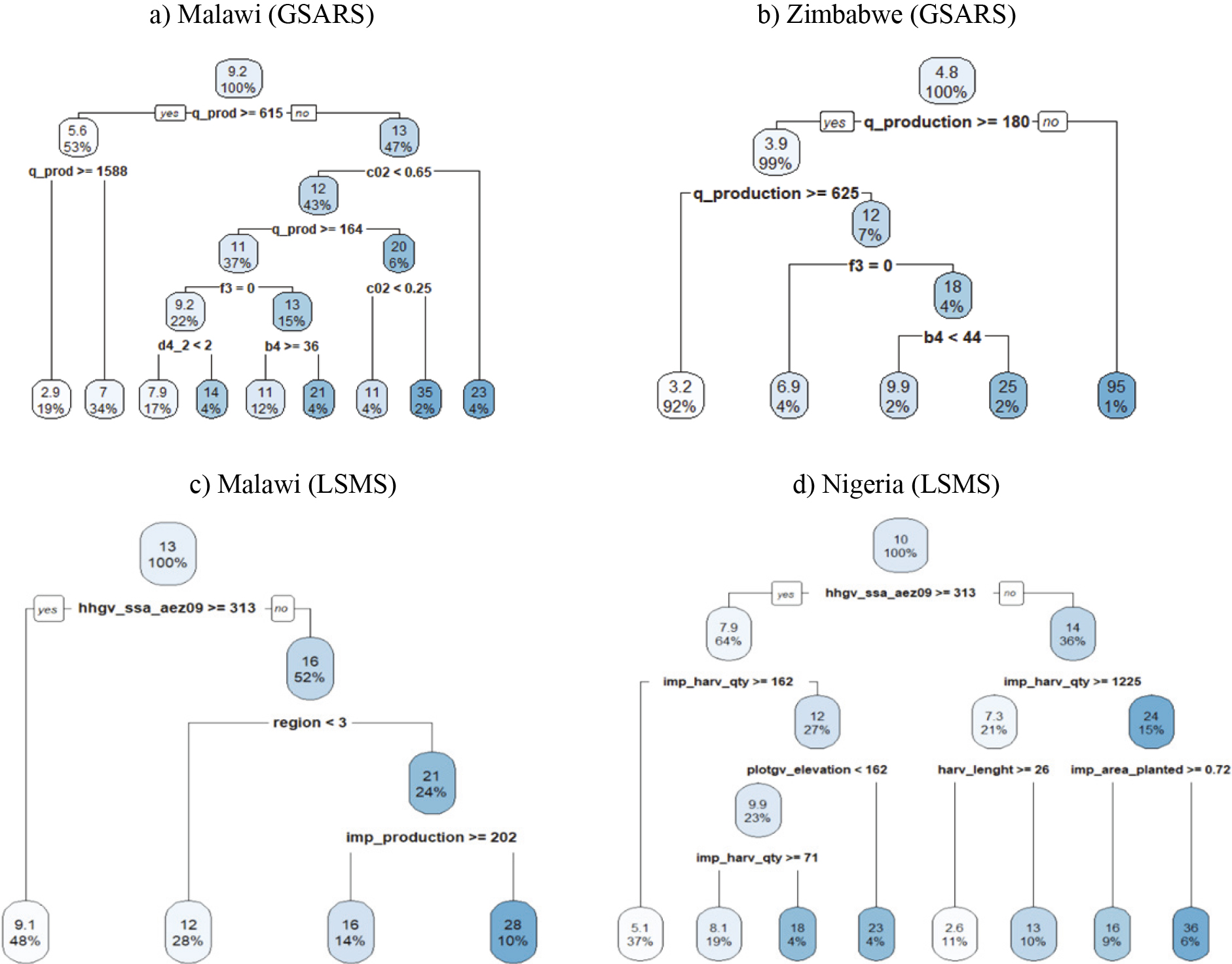
Figure 1.
Regression trees.
5.Results
5.1Food loss models estimated for Malawi, Zimbabwe and Nigeria
5.1.1Models obtained for the GSARS harvest and post-harvest loss surveys in Malawi and Zimbabwe
GSARS Malawi – maize
On the basis of sampling theory, the estimated percent loss of maize using data from the GSARS survey in Malawi is 8.66% harvest and post-harvest losses with a standard error of 0.514% (95% CI: 7.66, 9.67). One of the best theory-based model for this sample, that includes selected variables and some interactions, predicted a mean estimate of 8.39% loss with a standard error of 0.502 (95% CI: 7.41, 9.38).
To improve the efficiency of the estimator, a regression tree was built to generate post-stratification criteria to specify the loss model. The regression tree for the GSARS loss survey in Malawi is shown in Fig. 1 example (a). The regression tree selected eight cutting points on five variables, namely the quantity of maize produced (q_prod), the age of the household head (b4), the percent of the area harvested (c02), whether the household received any assistance from the government (f3), and the drying method used (d4_2). This tree generates nine terminal nodes with different mean percentage losses.
The classification established as post-stratification to generate a percent loss estimate was used as a predictor variable in a Poisson model. The output from this model is shown in Table 3.
Table 3
Model with CART classification as regressor for the Malawi GSARS survey
| Poisson regression | Number of obs | |||||
| Wald chi2(8) | ||||||
| Log pseudolikelihood | Prob | |||||
| % HPHL | Coefficient | Robust standard error |
|
| 95% LL | 95% UL |
| 2 | 0.875 | 0.163 | 5.36 | 0.00 | 0.555 | 1.195 |
| 3 | 0.943 | 0.206 | 4.59 | 0.00 | 0.540 | 1.346 |
| 4 | 1.346 | 0.292 | 4.61 | 0.00 | 0.773 | 1.919 |
| 5 | 1.328 | 0.193 | 6.88 | 0.00 | 0.950 | 1.707 |
| 6 | 1.930 | 0.244 | 7.91 | 0.00 | 1.452 | 2.409 |
| 7 | 1.377 | 0.355 | 3.88 | 0.00 | 0.682 | 2.073 |
| 8 | 2.234 | 0.218 | 10.23 | 0.00 | 1.806 | 2.662 |
| 9 | 1.850 | 0.237 | 7.8 | 0.00 | 1.386 | 2.315 |
| Constant | 1.097 | 0.147 | 7.44 | 0.00 | 0.808 | 1.386 |
This is a parsimonious model that uses only one classification variable as the predictor, but it includes three independent variables in the classification criteria. To test the use of a Poisson model (natural log as link function) and the specification of the model with respect to the independent classification variable, the corresponding linktest is shown in Table 4 example (a). This test indicates that the specified on-farm loss model shows very good functionality for estimating the mean percent losses, where the linear prediction
Table 4
Model specification tests, results from the linktests
| a) Malawi GSARS | b) Zimbabwe GSARS | ||||||
|---|---|---|---|---|---|---|---|
| Predictor | Coefficient | Std. Err. |
| Predictor | Coefficient | Std. Err. |
|
|
| 1.000 | 0.471 | 0.034 |
| 1.000 | 0.424 | 0.018 |
|
| 0.000 | 0.104 | 1.000 |
| 0.000 | 0.073 | 1.000 |
| c) Malawi IHS4 | d) Nigeria GHS 15/16 | ||||||
| Predictor | Coefficient | Std. Err. |
| Predictor | Coefficient | Std. Err. |
|
|
| 1.000 | 1.495 | 0.503 |
| 1.000 | 0.641 | 0.119 |
|
| 0.000 | 0.264 | 1.000 |
| 0.000 | 0.134 | 1.000 |
GSARS Zimbabwe – maize
The sampling-based estimate for the harvest and post-harvest percent loss of maize in Zimbabwe using the GSARS farm loss survey gives a mean on-farm loss of 4.0% with a standard error of 0.404% (95% CI: 3.2, 4.8). The same data-driven procedure was used to improve the mean estimate, where a regression tree was built to generate post-stratification criteria, as shown in Fig. 1 example (b). The regression tree selected four cutting points on three variables, namely: the quantity of maize produced (q_production), age of the household (b4), and whether the household received any assistance from the government (f3). This tree arrives at five terminal nodes used as stratification to generate a Poisson model; the output was omitted.
This model fits properly. It shows a good linear relationship for the predicted value
5.1.2Models obtained for the Malawi and Nigeria LSMS-ISA surveys
Malawi IHS4 – maize
The sampling base estimate for the percent loss of maize in Malawi, using data from the Living Standard Measurement Studies, showed a point estimate of 14.5% with a standard error of 0.661% (95% CI: 13.2, 15.8). To improve the efficiency of the estimator for the post-harvest percentage losses of maize, the regression tree for the post-stratification criteria was obtained. This is shown in Fig. 1 example (c).
The regression tree selected three cutting points on three variables: crop harvested production (imp_production), IHS4 2016 region location (region), and agro-ecological zone (hhgv_ssa_aez09). This tree arrives at four terminal nodes with different mean percentage losses. The Poisson model for this sample apparently fits properly, the linktest showing very good functionality in estimating the mean percentage of losses. Linear prediction
The estimated percentage loss of maize using this model is also 14.5% but with a slightly smaller standard error of 0.621% (95% CI: 13.3, 15.7). This represents an efficiency increase of only 12%. It is clear that the independent variables included in this model are not specific to harvesting procedures and refer to general aspects of production places, showing that recorded information is less related to food losses.
Nigeria GHS 2015/16 – maize
The sampling-based estimate for post-harvest percentage losses of maize in Nigeria for the LSMS-ISA dataset provides a mean food loss of 10.1% with a standard error of 0.978% (95% CI: 8.2, 12.0). Data-driven procedures to improve the mean estimate generated a regression tree with seven cutting points on five variables: agro-ecological zone (hhgv_ssa_aez09), area planted (imp_area_planted), harvested quantity (imp_harv_qty), harvest length in days on average (harv_lenght), and plot elevation (plplotgv_elevation). This tree, shown in Fig. 1 example (d), arrives at eight terminal nodes used as stratification to generate a Poisson model. The linktest for this model shows similar results (Table 4 example d), with a correspondence of 1:1 between the observed percentage of post-harvest food loss and the linear prediction
The estimated percentage loss of maize using this model is also 10.1% but with a smaller standard error of 0.8.23% (95% CI: 8.5, 11.7). This represents an efficiency increase of 29.1%.
5.2Results to reduce the sample size to a sub-sample and use the models to improve loss estimates
5.2.1Results obtained for the GSARS farm loss surveys in Malawi and Zimbabwe
GSARS Malawi – maize
To evaluate changes in the relative efficiency of food loss estimates based on a progressive sample size reduction by simulating a reduction of survey data collection, models on sub-samples were estimated using the regression tree stratification obtained from the full sample. Table 5 shows the simulated sample reduction and the corresponding estimates for the percentage food loss for maize based on survey theory estimates and the model-based estimates.
Table 5
Estimates, standard errors and relative efficiencies for sub-samples – Malawi GSARS
| Sample reduction | Survey-based loss estimate | Post-stratification loss estimate (model-based) | Model relative efficiency | ||
|
|
|
|
| ||
| 0% | 8.66 | 0.514 | 8.66 | 0.429 | 30.3% |
| 10% | 8.58 | 0.543 | 8.58 | 0.441 | 26.4% |
| 20% | 8.68 | 0.584 | 8.68 | 0.474 | 15.1% |
| 30% | 8.42 | 0.592 | 8.42 | 0.481 | 12.6% |
| 40% | 8.51 | 0.671 | 8.51 | 0.556 | |
| 50% | 8.34 | 0.720 | 8.34 | 0.619 | |
It is clear that with a sample reduction of 30%, the model estimate still presents good efficiency of 12.6% compared to the survey estimate using the whole sample, meaning that the use of models can help to improve food loss estimates with an important reduction in survey data collection. An alternative to sample reduction is to impute missing values to enhance model estimates. In Table 6, survey estimates and model-based estimates using imputed missing values on the reduced part of the sample are presented.
Table 6
Estimates, standard errors and relative efficiencies for imputed sub-samples – Malawi GSARS
| Sample reduction | Survey-based loss estimate | Estimates with model-based imputation | ||
|
|
|
|
| |
| 0% | 8.66 | 0.514 | 8.66 | 0.514 |
| 10% | 8.58 | 0.543 | 8.93 | 0.506 |
| 20% | 8.68 | 0.584 | 8.73 | 0.483 |
| 30% | 8.42 | 0.592 | 8.79 | 0.476 |
| 40% | 8.51 | 0.671 | 9.15 | 0.470 |
| 50% | 8.34 | 0.720 | 9.05 | 0.438 |
In this table, an important concern arises because the use of imputed samples reduces the standard errors
GSARS Zimbabwe – maize
The same application of sample reduction on the food loss model was used on maize for the Zimbabwe survey dataset. In Table 7, a sample reduction of 50% is achieved with the use of model estimates, obtaining a relative efficiency of 9.4% with respect to the whole sample survey estimate.
Table 7
Estimates, standard errors and relative efficiencies for sub-sample – Zimbabwe GSARS
| Sample reduction | Survey-based loss estimate | Post-stratification loss estimate (model-based) | Model relative efficiency | ||
|
|
|
|
| ||
| 0% | 3.98 | 0.404 | 3.98 | 0.259 | 59.1% |
| 10% | 4.09 | 0.450 | 4.09 | 0.277 | 53.1% |
| 20% | 3.85 | 0.429 | 3.85 | 0.298 | 45.7% |
| 30% | 3.80 | 0.447 | 3.80 | 0.310 | 41.1% |
| 40% | 3.87 | 0.508 | 3.87 | 0.347 | 26.3% |
| 50% | 3.99 | 0.572 | 3.99 | 0.384 | 9.4% |
The use of imputed missing values in reduced samples as an option is presented in Table 8. The same concern applies here about standard error reductions with imputed values which implies a greater risk of an increased probability of missing confidence interval estimates.
Table 8
Estimates, standard errors and relative efficiencies for imputed sub-samples – Zimbabwe GSARS
| Sample reduction | Survey-based loss estimate | Estimates with model-based imputation | ||
|
|
|
|
| |
| 0% | 3.98 | 0.404 | 3.98 | 0.404 |
| 10% | 4.09 | 0.450 | 3.85 | 0.352 |
| 20% | 3.85 | 0.429 | 3.96 | 0.356 |
| 30% | 3.80 | 0.447 | 3.92 | 0.356 |
| 40% | 3.87 | 0.508 | 3.81 | 0.323 |
| 50% | 3.99 | 0.572 | 3.98 | 0.345 |
Table 9
Estimates, standard errors and relative efficiencies for sub-samples – Malawi IHS4
| Sample reduction | Survey-based loss estimate | Post-stratification loss estimate (model-based) | Model relative efficiency | ||
|
|
|
|
| ||
| 0% | 14.52 | 0.661 | 14.52 | 0.621 | 12.0% |
| 10% | 14.58 | 0.700 | 14.58 | 0.656 | 1.5% |
| 20% | 14.32 | 0.741 | 14.32 | 0.699 | |
| 30% | 14.25 | 0.798 | 14.25 | 0.756 | |
| 40% | 13.79 | 0.837 | 13.79 | 0.777 | |
| 50% | 13.65 | 0.892 | 13.65 | 0.835 | |
5.2.2Results obtained for the Living Standard Measurement Studies in Malawi and Nigeria
Malawi IHS4 – maize
To evaluate changes in the relative efficiency of food loss estimates based on a progressive sample size reduction, in the LSMS-ISA from Malawi, Table 9 shows the results of sample-based and model-based percent loss estimates for simulated sub-samples.
In this case, the gains obtained from model-based estimates compared to sample-based estimates in the standard error are limited. This can be a result of the weak information related to on-farm loss determinants.
In Table 10, survey and model estimates using imputed missing values on the reduced part of the sample are shown. As mentioned above, imputation can drive us to artificially smaller standard errors.
Table 10
Estimates, standard errors and relative efficiencies for imputed sub-samples – Malawi IHS4
| Sample reduction | Survey-based loss estimate | Estimates with model-based imputation | ||
|
|
|
|
| |
| 0% | 14.52 | 0.661 | 14.52 | 0.661 |
| 10% | 14.58 | 0.700 | 14.37 | 0.626 |
| 20% | 14.32 | 0.741 | 14.26 | 0.586 |
| 30% | 14.25 | 0.798 | 13.98 | 0.538 |
| 40% | 13.79 | 0.837 | 14.42 | 0.521 |
| 50% | 13.65 | 0.892 | 13.86 | 0.470 |
Table 11
Estimates, standard errors and relative efficiencies for sub-sample – Nigeria GHS15/16
| Sample reduction | Survey-based loss estimate | Post-stratification loss estimate (model-based) | Model relative efficiency | ||
|
|
|
|
| ||
| 0% | 10.10 | 0.978 | 10.10 | 0.823 | 29.1% |
| 10% | 9.85 | 1.024 | 9.85 | 0.866 | 21.6% |
| 20% | 10.17 | 1.122 | 10.17 | 0.959 | 3.8% |
| 30% | 9.76 | 1.111 | 9.76 | 0.954 | 4.7% |
| 40% | 8.75 | 0.997 | 8.75 | 0.869 | 21.0% |
| 50% | 9.36 | 1.154 | 9.36 | 1.018 | |
Table 12
Estimates, standard errors and relative efficiencies for imputed sub-sample – Nigeria GHS15/16
| Sample reduction | Survey-based loss estimate | Estimates with model-based imputation | ||
|
|
|
|
| |
| 0% | 10.10 | 0.978 | 10.10 | 0.978 |
| 10% | 9.85 | 1.024 | 9.39 | 0.877 |
| 20% | 10.17 | 1.122 | 9.26 | 0.852 |
| 30% | 9.76 | 1.111 | 9.58 | 0.835 |
| 40% | 8.75 | 0.997 | 9.49 | 0.781 |
| 50% | 9.36 | 1.154 | 10.12 | 0.773 |
Nigeria GHS 2015/16 – maize
Sample-based and model-based estimates for post-harvest loss percentage for maize on the LSMS-ISA dataset is shown in Table 11.
It can be seen that in the case of Nigeria, compared to Malawi (previously shown), the gains in the standard error by using the food loss model are more relevant, achieving at least a similar relative efficiency with a sample reduction of 20–30%. In Table 12, survey and model-based estimates using imputed missing values on the reduced part of the sample are shown.
Model-based estimates using imputation procedures are not recommended for improving loss estimates, because of the risk derived from artificial error reduction.
6.Discussion
The use of modelling approaches to support sub-sampling strategies for on-farm loss data collection shows an overall positive result, where loss models built from post-stratification and the Classification and Regression Tree Method show sufficiently good prediction performance and efficiency gains on mean estimates. The datadriven post-stratification models improve loss estimates obtained from full sampling and sub-sampling compared to the sample-based estimates. Sub-sampling is thereby possible, without a considerable loss in the quality of the estimates and the models provide some scope for further reductions of the sub-sample.
These results are stronger for the GSARS farm loss survey datasets compared to the LSMS-ISA survey data, which is to some extent related to the specific survey design used in the GSARS farm loss survey that builds on a detailed assessment of food losses. On the other hand, the GSARS farm loss survey was conducted on a sub-national level, covering a less heterogeneous population compared to nationwide LSMS-ISA surveys. The set of variables that were chosen to specify the classification groups follow the general knowledge of on-farm loss causes, where smallscale farmers tend to have higher loss percentages compared to largescale producers. Production levels are therefore a structural variable that overly may signal efficiency of harvest and post-harvest procedures. Socio-economic variables such as the age of the producer, provide additional criteria for explaining on-farm loss differences, with older farmers facing higher losses. Access to technical assistance and drying methods used are other relevant variables found to specify the model. Apart from those chosen by the CART method, other variables from the GSARS farm loss survey were found to be relevant to explaining farm losses, such as storage technology, use of pesticides during storage, days of harvesting, and harvest methods. These are aligned to the literature review and were identified when testing the theory-based farm loss models but are less relevant for prediction purposes.
For the LSMS-ISA surveys, the model application in the case of Malawi resulted in little improvements obtained from modelling on the loss estimate, while the model-based estimations for Nigeria showed considerable improvements. It is therefore important to highlight the need for good quality data to obtain the expected gains from the use of the modelling approach. In the case of Malawi, the sample is spread over a twelve-month period and the recall period varies substantially within the sample in the event that the fieldwork is completed after several months after the harvest period, while in Nigeria, two visits are undertaken close to the planting and harvest periods. The shorter periods between the survey and the harvesting period in the Nigeria survey are likely to contribute to more accurate responses [47, 48, 49].1010 The results obtained for the LSMS-ISA survey in Nigeria show that the modelling approach works on national surveys, although these might not focus on food loss measurement as the main survey objective and are therefore composed of a wider but less loss-specific set of variables. It is interesting to observe, that, apart from production quantities and area planted, the region and agro-ecological zone, as well as the plot characteristics account for most of the effects identified in the CART Method for prediction purposes. These are valuable insights for the set of relevant variables to be included in farm surveys, a conclusion supported by the literature review and a difference to the GSARS surveys where these have not been collected or included in the available datasets.
The applications with respect to model-based imputation procedures to extrapolate the estimates from the sub-sample to the full sample show that its use is limited for improvements of on-farm loss estimates. Model-based imputations above 10% of sample-size reduction started to show an artificial reduction of the standard error of the full sample. Therefore, the model-based imputation should not be applied to extrapolate larger datasets. The artificial reduction of standard errors can result in potential errors in the use of confidence intervals, representing a risk for decision making. Overall, model-based imputations showed better results than median-based imputations and can therefore be used as a complement to fill possible non-responses.
Some relevant conclusions can be derived from the information that can support farm loss modelling on sub-samples and are therefore recommended to be considered in survey design and implementation. As suggested in the 50x2030 Initiative sampling guidelines [10], sub-sampling for the on-farm loss module in household and farm surveys is recommended for optimizing data collection costs. The saved resources could then be invested in a more precise assessment of losses, either by detailing declarations or by using other objective methods to improve the estimates. Indeed, for the given surveys, a more detailed loss module seems to provide better loss estimates and avoids unreliable zero-response rates, an area where further research is needed. Investments in better quality data with a reduced sample size also pay off in stronger loss models, which in turn helps to sustain the sub-sampling strategy. Finally, geo-references from LSMS-ISA are shown to be very useful for adding climate and plot characteristics to the survey data which in turn can be relevant to building farm loss models. Thus, given the minimal implementation burden for the enumerators, capturing GPS coordinates of the surveyed household/dwelling and plots is highly recommended.
Recognizing, on the one hand, the importance of collecting data on losses to inform policymaking, and, on the other hand, the complexity of collecting such data, the results highlight possible gains from the integration of survey data with modelling to improve the quality of loss estimates and support sub-sampling strategies. The combination of sub-sampling a detailed module on post-harvest losses with a modelling approach can be a useful recommendation in largescale household and farm surveys, and through this approach, the 50x2030 Initiative can represent the ideal opportunity for scaling-up the collection of data on post-harvest losses.
Notes
1 For more on the 50x2030 Initiative to Close the Agricultural Data Gap see 50x30 Initiative (2021a).
2 In this document harvest and post-harvest losses are defined as the losses occurring on the farm from harvest to storage. More specifically, losses as defined in this manuscript include losses during harvesting, post-harvest operations (depending on the crop, this would include threshing/shelling, cleaning/winnowing, and drying, peeling, washing and slicing). Losses also include on-farm transport, and storage at farm level.
3 A detailed description of the HPHL-AG questionnaire and its integration into the 50x2030 modular survey system can be found: https://www.50x2030.org/resources/survey-instruments.
4 For further detail see: “Integrated sampling design for agricultural and socio-economic surveys: overview and application in Uganda Harmonized Integrated Survey” by Dramane Bako, Marcello D’Orazio, Silvia Missiroli, Vincent Fred Ssennono, Chiara Brunelli, Talip Kilic, Giulia Ponzini, Flavio Bolliger of this SJIAOS 50x2030 Special Section (Vol. 38 (2022), issue 1).
6 Global Strategy to Improve Agricultural and Rural Statistics (GSARS).
7 The microdata, survey report and basic information document about the GHS 2015/16 implementation are available: https://micro data.worldbank.org/index.php/catalog/2936.
8 The microdata, survey report and basic information document about the GHS 2015/16 implementation are available: https://micro data.worldbank.org/index.php/catalog/2734.
9 The efficiency increase or “model relative efficiency” is the percentual difference between the standard error obtained from the sample-based loss estimate on the full sample to the standard error obtained from the model-based loss estimates on the full sample and any size of the sub-samples.
References
[1] | United Nations General Assembly. Transforming our world: the 2030 Agenda for Sustainable Development. Resolution A/RES/70/1. New York: United Nations; 21 October (2015) . |
[2] | Food and Agriculture Organization. The State of Food and Agriculture. Moving forward on food loss and waste reduction. Rome: FAO; (2019) . http://www.fao.org/3/ca6030en/ca6030en.pdf. |
[3] | Kitinoja L, Tokala VY, Brondy A. Challenges and opportunities for improved postharvest loss measurements in plant-based food crops. Journal of Postharvest Technology. (2018) ; 6: (4): 16–34. |
[4] | Xue L, Liu G, Parfitt J, Liu X, Van Herpen E, Stenmarck Å, O’Connor C, Östergren K, Cheng S. Missing food, Missing data? A critical review of global food losses and food waste data. Environmental Science & Technology. (2017) ; 51: (12): 6618–6633. |
[5] | Delgado L, Schuster M, Torero M. The reality of food losses: A new measurement methodology. IFPRI Discussion Paper 1686. Washington, DC: International Food Policy Research Institute; (2017) . http://ebrary.ifpri.org/cdm/ref/collection/p15738coll2/id/131530. |
[6] | Delgado L, Schuster M, Torero M. Quantity and quality food losses across the value chain: A comparative analysis. Food Policy. (2020) ; 98. doi: 10.1016/j.foodpol.2020.101958. |
[7] | Johnson LK, Dunning RD, Bloom JD, Gunter CC, Boyette MD, Creamer NG. Estimating on-farm food loss at the field level: A methodology and applied case study on a North Carolina farm. Resources, Conservation and Recycling. (2018) ; 137: : 243–250. doi: 10.1016/j.resconrec.2018.05.017. |
[8] | Global Strategy to improve Agricultural and Rural Statistics (GSARS). Guidelines on the measurement of harvest and post-harvest losses. Rome: FAO; (2018) . |
[9] | 50x2030 Data Initiative. The 50x2030 Initiative: Bringing together committed partners to fill the agricultural data gap. Rome: World Bank; (2021) . |
[10] | 50x2030 Data Initiative. The 50x2030 Initiative: A guide to sampling. Rome: World Bank; (2021) . |
[11] | Venrick EL. The statistics of subsampling. Limnol. Oceanogr. (1971) ; 16: : 811–818. |
[12] | Kumar DK, Basavaraja H, Mahajanshetti SB. An economic analysis of post-harvest losses in vegetables in Karnataka. Indian Journal of Agricultural Economics, Indian Society of Agricultural Economics. (2006) ; 61: (1): 1–13. |
[13] | Basavaraja H, Mahajanashetti SB, Udagatti NC. Economic analysis of post-harvest losses in food grains in India: A case study of Karnataka. Agricultural Economics Research Association (India). (2007) ; 20: (1). |
[14] | Begum M, Hossain M, Papanagiotou E. Economic analysis of post-harvest losses in food-grains for strengthening food security in northern regions of Bangladesh. International Journal of Applied Research in Business Administration and Economics. (2012) ; 1: (3): 56–65. |
[15] | Khatun M, Karim MR, Khandoker S, Hossain TMB, Hossain S. Post-harvest loss assessment of tomato in some selected areas of Bangladesh. International Journal of Business, Social and Scientific Research. (2014) ; April-June 1(3): 209–218. |
[16] | Arun GC, Ghimire K. Estimating post-harvest loss at the farm level to enhance food security: A case of Nepal. Int J Agric Environ Food Sci. (2019) ; 3: (3): 127–136. doi: 10.31015/jaefs.2019.3.3. |
[17] | Paneru R, Paude GP, Thapa R. Determinants of post-harvest maize losses by pests in mid hills of Nepal. International Journal of Agriculture, Environment and Bioresearch. (2018) ; 3: (1). |
[18] | Adisa RS, Adefalu LL, Olatinwo LK, Balogun KS, Ogunmadeko OO. Determinants of post-harvest losses of yam among yam farmers in Ekiti State, Nigeria. Bulletin of the Institute of Tropical Agriculture, Kyushu University. (2015) ; 38: (1): 73–78. doi: 10.11189/bita.38.073. |
[19] | Babalola DA, Oyekanmi. Determinants of postharvest losses in tomato production: A case study of Imeko – Afon local government area of Ogun state. Journal of Life and Physical Science. (2010) ; acta SATECH 3(2): 14–18. |
[20] | Tadesse B, Bakala F, Mariam L. Assessment of postharvest loss along potato value chain: The case of Sheka Zone, southwest Ethiopia. Agric & Food Secur. (2018) ; 7: : 18. doi: 10.1186/s40066-018-0158-4. |
[21] | Ambler K, Brauw A, Godlonton S. Measuring postharvest losses at the farm level in Malawi. Australian Journal of Agricultural and Resource Economics. (2018) ; 62: (1): 139–160. doi: 10.1111/1467-8489.12237. |
[22] | Folayan JA, Babalola JA, Ilesa A. Determinants of Post Harvest Losses of Maize in Akure North Local Government Area of Ondo State, Nigeria Journal of Sustainable Society. (2013) ; 2: (1). doi: 10.11634/216825851403289. |
[23] | Aidoo R, Rita A, Osei Mensah J. Determinants of postharvest losses in tomato production in the Offinso North District of Ghana. Journal of Development and Agricultural Economics. (2014) ; 6: (8): 338–344. doi: 10.58797/JDAE2013.0545. |
[24] | Huang T, Li B, Shen D, Cao J, Mao B. Analysis of the grain loss in harvest based on logistic regression. Procedia Computer Science. (2017) ; 122: : 698–705. doi: 10.1016/j.procs.2017.11.426. |
[25] | Ansah I, Tetteh B. Determinants of yam postharvest management in the Zabzugu District of Northern Ghana. Advances in Agriculture. (2016) . Article ID 9274017. 9 pages. doi: 10.1155/2016/9274017. |
[26] | Hossain M, Miah MA. Post-harvest losses and technical efficiency of potato storage systems in Bangladesh. National Food Policy Capacity Strengthening Programme. Final Report CF # 2/08. (2009) . |
[27] | Shee A, Mayanja S, Simba E, Stathers T, Bechoff A, Bennett B. Determinants of postharvest losses along smallholder producers maize and sweetpotato value chains: An ordered Probit analysis. Food Security. (2019) ; 11: (2). doi: 10.1007/s12571-019-00949-4. |
[28] | Garikai M. Assessment of vegetable postharvest losses among smallholder farmers in Umbumbulu area of KwaZulu-Natal province. Master’s Thesis, University of KwaZulu-Natal, Pietermaritzburg, South Africa. (2014) . http://hdl.handle.net/10413/11918. |
[29] | Amentae T, Tura EG, Gebresenbet G, Ljungberg D. Exploring value chain and post-harvest losses of Teff in Bacho and Dawo districts of central Ethiopia. Journal of Stored Products and Post-harvest Research. (2016) ; 7: (1): 11–28. doi: 10.5897/JSPPR2015.0195. |
[30] | Falola A, Salami M, Bello A, Olaoye T. Effect of yam storage techniques usage on farm income in Kwara State, Nigeria. Agrosearch. (2017) ; 17: (1): 54–65. doi: 10.4314/agrosh.v17i1.5. |
[31] | Kikulwe E, Okurut S, Ajambo S, Id K, Nowakunda, Stoian D, Naziri D. Postharvest losses and their determinants: A challenge to creating a sustainable cooking banana value chain in Uganda. Sustainability. (2018) ; 10: (7): 2381. doi: 10.3390/su10072381. |
[32] | Kimenju S, De Groote H. Economic analysis of alternative maize storage technologies in Kenya. Paper presented at the Third Conference of the African Association of Agricultural Economists (AAAE). (2010) . September 19–23; Cape Town, South Africa. http://econpapers.repec.org/scripts/search/search.asp?ft=simon+kimenju. |
[33] | Qu X, Kojima D, Nishihara Y, Wu L, Ando M. Impact of rice harvest loss by mechanization or outsourcing: Comparison of specialized and part-time farmers. Agric. Econ. – Czech. (2020) ; 66: : 542–549. doi: 10.17221/253/2020-AGRICECON. |
[34] | Alidu A-F, Ali E, Aminu H. Determinants of post harvest losses among tomato farmers in the Navrongo Municipality in The Upper East Region. Journal of Biology, Agriculture and Healthcare. (2016) ; 6: (12). |
[35] | Mebratie MA, Haji J, Woldetsadik K, Ayalew A. Determinants of postharvest banana loss in the marketing chain of Central Ethiopia. Food Science and Quality Management. (2015) ; 37: : 52–63. |
[36] | Maziku P. Determinants for post-harvest losses in maize production for small holder farmers in Tanzania, African Journal of Applied Research. (2019) ; 5: (1): 1–11. doi: 10.26437/ajar.05.01.2019.01. |
[37] | Kwami M, Kamarulzaman N, Morris K. Small-scale postharvest practices among plantain farmers and traders: A potential for reducing losses in rivers state, Nigeria. Scientific African. (2019) ; 4: : e00086. doi: 10.1016/j.sciaf.2019.e00086. |
[38] | 50x2030 Initiative. Literature review on on-farm post-harvest loss models. Rome: World Bank; forthcoming. |
[39] | Breiman L, Friedman JH, Olshen RA, Stone CJ. Classification and regression trees (1st ed.). Routledge; (1984) . doi: 10.1201/9781315139470. |
[40] | Loh WY. Classification and regression trees. Wiley Interdiscip. Rev. Data Min. Knowl. Discov. (2011) ; 1: (1): 14–23. |
[41] | Smith TMF. Post-Stratification. Journal of the Royal Statistical Society. Series D (The Statistician). (1991) ; 40: (3): 315–23. doi: 10.2307/2348284. |
[42] | Pregibon D. Goodness of link tests for generalized linear models. Journal of the Royal Statistical Society. Series C (Applied Statistics). (1980) ; 29: (1): 15–14. doi: 10.2307/2346405. |
[43] | Food and Agriculture Organization (FAO). Guidelines on the measurement of harvest and post-harvest losses. Estimation of crop harvest and post-harvest losses in Malawi. Maize, rice and groundnuts. Field Test Report. Rome: FAO; (2020) . www.fao.org/3/cb1562en/cb1562en.pdf. |
[44] | Food and Agriculture Organization (FAO). Guidelines on the measurement of harvest and post-harvest losses. Estimation of crop harvest and post-harvest losses in Zimbabwe. Field Test Report. Rome: FAO; (2020) . |
[45] | Wossen T, Abdoulaye T, Alene A, Nguimkeu P, Feleke S, Rabbi IY, Haile MG, Manyong V. Estimating the productivity impacts of technology adoption in the presence of misclassification. American Journal of Agricultural Economics. (2019) ; 101: : 1–16. doi: 10.1093/ajae/aay017. |
[46] | Wineman A, Njagi T, Anderson CL, Reynolds TW, Alia DY, Wainaina P, Njue E, Biscaye P, Ayieko MW. A case of mistaken identity? Measuring rates of improved seed adoption in Tanzania using DNA fingerprinting. J Agric Econ. (2020) ; 71: : 719–741. doi: 10.1111/1477-9552.12368. |
[47] | Wollburg P, Tiberti M, Zezza A. Recall length and measurement error in agricultural surveys. Food Policy. (2020) ; 100: : 102003. doi: 10.1016/j.foodpol.2020.102003. |
[48] | Kilic T, Moylan HG, Ilukor J, Mtengula C, Pangapanga-Phiri I. Root for the tubers: Extended-harvest crop production and productivity measurement in surveys. Food Policy. (2021) ; 102. doi: 10.1016/j.foodpol.2021.102033. |
[49] | Deininger K, Carletto C, Savastano S, Muwonge J. Can diaries help in improving agricultural production statistics? Evidence from Uganda. Journal of Development Economics. (2012) ; 98: : 42–50. |


