Identifying and evaluating COVID-19 effects on short-term statistics

3.2.1Anticipated effects

We expected that the survey response rates and the VAT reporting rates might be reduced during periods with COVID-19 measures since entrepreneurs were expected to have other priorities than reporting data to external agencies.

3.2.2Measures

The CBS data collection department (DVZ) has a standard procedure to get high response rates for the STS. Enterprises that have to provide quarterly survey data receive at the beginning of each quarter registered letters and emails with access codes to online questionnaires. They have approximately one month to fill in those questionnaires about data of the previous quarter. The enterprises will receive a number of reminders via letters or electronically. From approximately 40 days after the date on which the registered letter/email was sent, DVZ can, besides sending reminder letters or emails, also call enterprises to increase response rates. Here, a top-down approach is used to ensure that the most influential enterprises are approached first. If enterprises still do not respond, an enforcement policy will be in place in which companies could potentially get fined for not sending data. For enterprises that have to provide monthly survey data, a similar approach is followed. They will receive registered letters/emails at the end of each month and a last reminder will be sent approximately 20 days after the date on which the registered letter/email was sent.

During the lockdowns, for STS, contacting by email and by phone was preferred over sending letters since DVZ anticipated that entrepreneurs whose enterprises were inactive or whose shops were closed would miss letters sent to them. Furthermore, the enforcement policy was put on hold.

Moreover, for industries in retail trade the date of starting with processing the response was advanced, and the output figures were published two weeks earlier than normal. Enterprises in those industries were actively contacted by phone and were asked to deliver their STS data earlier than normal. Some of the employees of DVZ that could not do their regular work due to COVID-19 situation were deployed to call those enterprises.

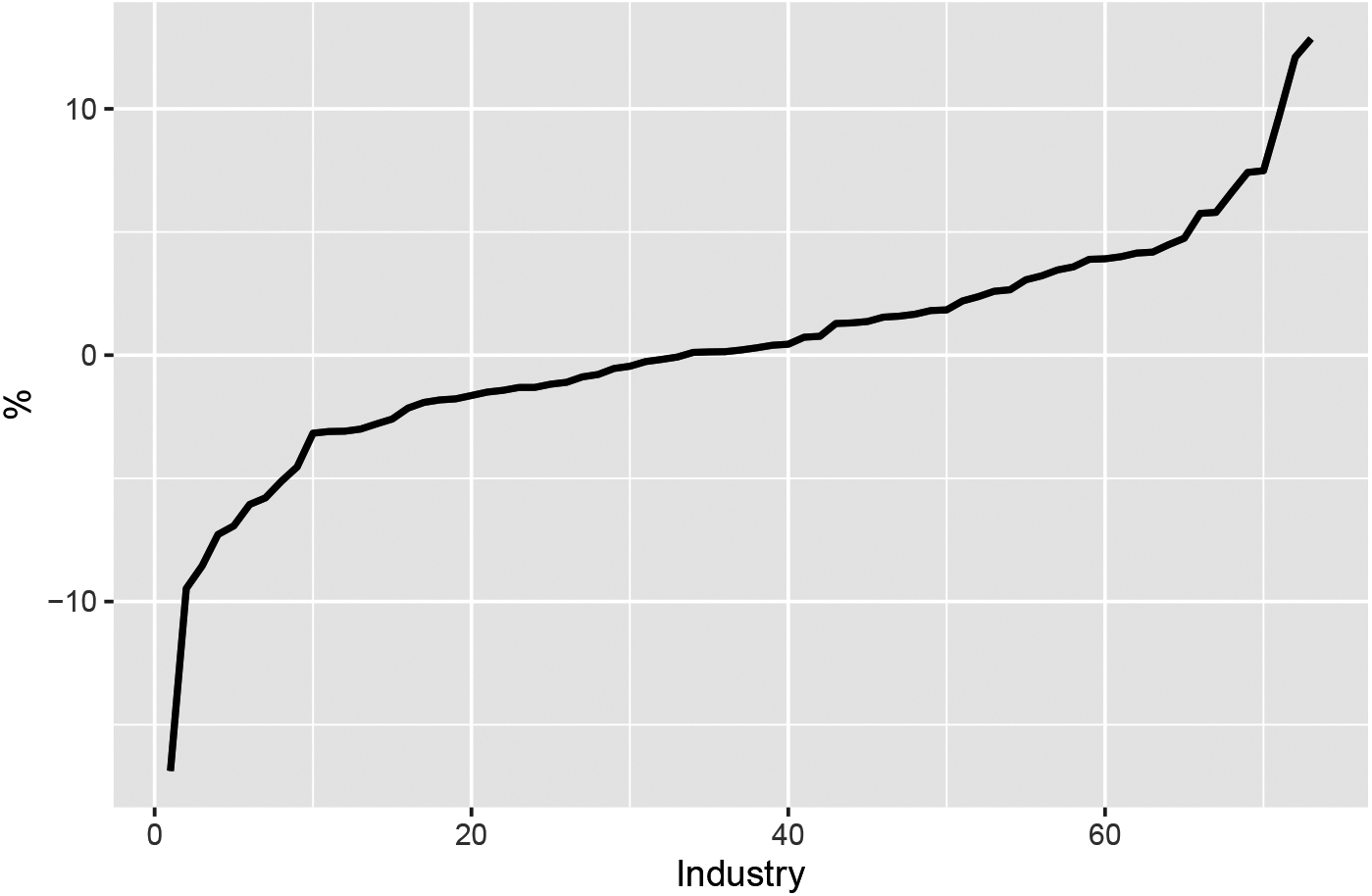
Figure 1.

Difference in turnover response rates per industry for the early estimates of the monthly STS statistics (SSD system) between the second quarter of 2020 (first lockdown) and the second quarter of 2019 (no lockdown). The 73 industries are sorted from small to large values.

3.2.3Results

We monitored whether the survey response rates were indeed lower than normal. We computed the turnover response rates for period t and industry k, denoted by ℛkt, given by:

where ak⁢it denotes whether unit i of industry k in period t has responded (ak⁢it=1) or not (ak⁢it=0), Y˙k⁢it denotes an observed turnover, Y~k⁢it denotes an imputed turnover, dk⁢it denotes the weight of the unit which is usually the inverse of the inclusion probability but it may be adjusted in the case of an outlier, and nkt denotes the sample size. The response rates also depended on the actual release, but to simplify the notation we did not explicitly include the release in the notation of ℛkt in Eq. (1).

The turnover response rates for the early estimates (published around 30 days after the end of the period) of the STS statistics of different economic sectors produced with the SSD system in pre-COVID-19 months were 86% or higher (see Table 3). During the first lockdown period (March-June 2020), the response rate for the early estimates remained at a high level and in some sectors it even slightly increased, see Table 3.

Figure 1 shows the difference in turnover response rate per industry for early estimates of the monthly turnover statistics for the second quarter of 2020 (lockdown) and the second quarter of 2019 (no lockdown). For most industries the difference in response rates was at most 5 percentage points. Only a few industries have a decline in turnover response rate larger than 5 percentage points. One industry had an increased response rate of 13 percentage points during the first lockdown. Note that some of the industries are small and their turnover response rates varied considerably from quarter to quarter depending on whether the larger enterprises already responded or not.

The turnover response rates for the quarterly estimates produced by the CCD system were also analysed. In the CCD system turnover values were imputed for all units with missing response. Hence, for the CCD system, the weights dk⁢it in Eq. (1) are equal to 1 and nkt stands for all units of the population. Whereas the turnover response rates for the early estimates remained at the same level for the monthly survey data (SSD system), a decline in response rates for the early estimates was seen for both the VAT-data and the quarterly survey data (CCD system). The decline for the first quarter of 2020 as compared to the first quarter of 2019 was of the order of 10% over all industries. Note that whereas only a small part of the first quarter of 2020 coincides with the first lockdown period, the data collection period for data on the first quarter of 2020 was during the middle of the first lockdown period. A smaller decline in response rates was seen for the second quarter of 2020 (compared to the second quarter of 2019). The 10% decline in response rate for the early estimates in the first quarter of 2020 did not cause a problem with the total amount of response because, averaged over all industries in the CCD system, still 60% of the total turnover was based on response. Furthermore, before publishing the Quarterly National Accounts that were based on the early STS-estimates, CBS checked that the updated CCD-estimates from a couple of days later (based on far more response), did not differ too much from the early estimates. Although the size of the response for the early estimates was sufficient for both the SSD and CCD system, we were aware of the risk that the early response during periods of a lockdown may be selective; that issue is addressed in Section 3.4.

In conclusion, it turned out that the turnover response rates for the early estimates of the SSD system were at similar or even slightly higher levels compared to non-COVID-19 periods; also for industries affected by the COVID-19 crisis (see Table 1 for those industries). CBS mentioned the importance of figures for society in the first letter (email) that they sent to the enterprises. Perhaps this has promoted them to sent in a response. However, a decline in response rate was seen for both the VAT data and the quarterly survey data for the CCD system. It is unclear to us why response rates of survey data of monthly published industries in the SSD systems remained high while response rates of survey data used in the CCD system for quarterly published surveys were somewhat reduced. What is clear is that additional efforts for the retail trade statistics worked out well and allowed us to accelerate the output.

Statistics Portugal (Moreira et al. [7]) who did not report additional measures with respect to the data collection, found a drop in their response rates on monthly business surveys of approximately 10% in April and May 2020 as opposed to 2019. Statistics Slovenia (Šuštar Kožuh [8]) gradually shifted to electronic communication with businesses, hardly used any reminders but extended the deadlines for data transmission for their STS. They found the monthly STS response in 2020 to be close to the response rates in 2019.

3.3.1Anticipated effects

Before explaining the anticipated effects, we first briefly introduce the usual editing score function. CBS uses different score functions to identify enterprises within the STS whose turnover values are influential and possibly incorrect. The most important score function, denoted by Ak⁢it,r, is based on influential growth rates. For the SSD system this score function is defined by:

where Yk⁢it and Yk⁢ir denote the reported or imputed value for the target variable (mostly total turnover) of enterprise i in industry k for the current period t or reference period r respectively, dk⁢it and dk⁢ir are the corresponding weights in the current and reference period respectively, and nkr stands for the number of sampling units in reference period r and industry k. Furthermore, Ykr stands for the weighted summed industry turnover. For the CCD system Ykr refers to the summation over all units in the population and the weights dk⁢it and dk⁢ir are equal to 1.

Enterprises that are entering and those that are leaving industry k have a zero turnover value for the period that they are not present in industry k. To better understand Ak⁢it,r as an editing score function we can rewrite Eq. (3.3.1) as (assuming dk⁢ir⁢Yk⁢ir≠0):

The symbol ωk⁢ir stands for the proportion of the weighted turnover of enterprise i to the weighted summed industry turnover, which is the influence component of the score function. Further, Gˇk⁢it,r is the weighted growth factor. The term (Gˇk⁢it,r-1) stands for the risk component of the score function, the extent to which the unit is outlying. Note that the sum of Ak⁢it,r over all enterprises within the industry yields ∑i=1nkt,rdk⁢it⁢Yk⁢it-dk⁢ir⁢Yk⁢irYkr=Gkt,r-1 with Gkt,r≡YktYkr, Ykt≡∑i=1nktdk⁢it⁢Yk⁢it, nkt stands for the sample size in period t and nkt,r stands for the size of the union of units in the sample for period t and r.

In practice, the previous period was used as reference period: r=t-1. Normally, an extreme absolute value of Ak⁢it,r indicates that the corresponding unit is an outlier and influential. However, a large absolute value of Ak⁢it,r is not necessary a indication for an outlier during lockdown. We anticipated that the absolute values of the score function Ak⁢it,r might increase greatly for many enterprises during lockdown since many enterprises will show a large turnover drop. We therefore expected Ak⁢it,r to be less suitable for finding outliers during lockdown.

3.3.2Measures

Since the score function Ak⁢it,r was less suitable during the lockdown periods, analysts put more emphasis on scatterplots rather than on Ak⁢it,r to identify outliers for the monthly industries that where seriously affected by the lockdown. In the scatterplots Yk⁢ir was plotted against Yk⁢it with r=t-1 or r=t-12. For the estimates made during 2020 this was the main measure taken, due to time limitations.

By the time the data pertaining to all months of 2020 were available in SSD, we had calculated a new editing score function to identify influential outliers that replaced Ak⁢it,r. This new editing score function was used in production from the spring of 2021 onwards. The first estimates for which is was used, were the final estimates over the reporting year 2020.

This alternative score function, denoted by Bk⁢it,r, aims to capture whether the growth of an enterprise is extreme relative to the average growth of the enterprises in the same industry. This score function is defined as

with Y´k⁢it≡Yk⁢ir⁢Gkt,r and the growth factor Gkt,r≡Ykt/Ykr. We can rewrite Eq. (3) (assuming dk⁢irYk⁢ir≠0) as:

where Gˇk⁢it,r and ωk⁢ir are defined in the second line of Eq. (3). Compared to Eq. (3) the term (Gˇk⁢it,r-1) is replaced by (Gˇk⁢it,r-Gkt,r). The difference G˘k⁢it,r-Gkt,r stands for the (new) risk component. Note that ∑i=1nkt,rBk⁢it,r=0.

3.3.3Results

The alternative scores Bk⁢it,r (see Section 3.3.2), with r=t-1, were used for editing of the data of Manufacturing and Retail Trade within the SSD system. When reviewing the STS for the reporting year 2020 (in the spring of 2021), a list of alternative scores was sent to analysts and validators of Manufacturing and Retail trade. They found that these scores were particularly interesting if turnover changes were mainly caused by a homogeneous group of units. Normally, all units with the usual score function |Ak⁢it,r|> 0.01 were checked: in the second quarter of 2020 this concerned 313 units for Manufacturing and 438 for Retail trade, see Fig. 2. The alternative score function |Bk⁢it,r|> 0.01 concerned 283 enterprises for Manufacturing and 372 for Retail trade, so those numbers were somewhat smaller. Some units were outlying according to |Ak⁢it,r|> 0.01 but not according to |Bk⁢it,r|> 0.01 and vice versa, see Fig. 2.

Figure 2.

Number of units with |Ak⁢it,r| and/or |Bk⁢it,r|>0.01 (score functions abbreviated as A and B in the figure) summed over April, May and June 2020, using the previous month as reference period, for Manufacturing and Retail trade.

At the time of writing this paper, CBS is still in the process of evaluating and perhaps improving the editing score function.

3.4.1Anticipated effects

Missing turnover values in the STS are imputed by using a ratio imputation of the form:

where Y~it denotes the imputed turnover value of enterprise i for period t, X stands for an auxiliary variable and Ydt/Xd is the ratio of the weighted total of Y for domain d in period t and the corresponding domain total for X. The domain d stands for a group of enterprises that are similar to unit i (based on the values of background variables such as size class and industry) and that hopefully have a similar Y/X ratio to unit i (on average over imputations). In most cases the chosen auxiliary variable X is the turnover in a reference period r in which case the equation is equivalent to Y~it=Yir⁢(Ydt/Ydr). For new enterprises (births) the number of employees in period t is often used as auxiliary variable.

There are three points of attention with respect to the imputation (Van Bemmel and Goorden [9]):

We anticipated that the setting and cancelling of COVID-19 measures would result in large changes of growth rates in STS that may in turn impact the quality of the imputations of STS:

We took the following measures:

3.4.2A measure for heterogeneity change

As a starting point for developing a measure for heterogeneity change, we used some results from Van Delden and Scholtus [10] who made a regression of survey turnover, denoted by yi to VAT turnover, denoted by xi. They found that the variance of the residuals of yi increased with the value of xi: Var⁢(ϵi)=σ2⁢(xi)λ, where ϵi stands for the residual and σ2 stands for a constant, see also Kutner et al. [11, pp. 424–431] on how to model heteroscedasticity. Van Delden and Scholtus [10] estimated λ and found λ^=1 to be a good estimate for different economic sectors, see also their Figs 3–6. Given this model for the heteroscedasticity, we assumed that the ratio of the standard deviation of the turnover values Yd⁢it in a domain d for period t over its mean (to the power α=λ/2, with λ^=1), Std⁢(Yd⁢it)/(Y¯dt)α, with Y¯dt≡(1/ndt)⁢∑i=1ndtYd⁢it, is relatively constant over time for a given domain. We refer to this ratio as the relative standard deviation of turnover of domain d and period t, denoted by RSD⁢(Yd⁢it). For different populations (domains) however we expected different values for RSD⁢(Yd⁢it).

Figure 3.

Relative Standard Deviation of eleven NACE codes in Retail trade from the first quarter of 2015 (period 1) till the forth quarter of 2016 (period 8). Growth factors are year-on-year. NACE codes are ending with ‘X’ when several underlying 5-digit codes are combined.

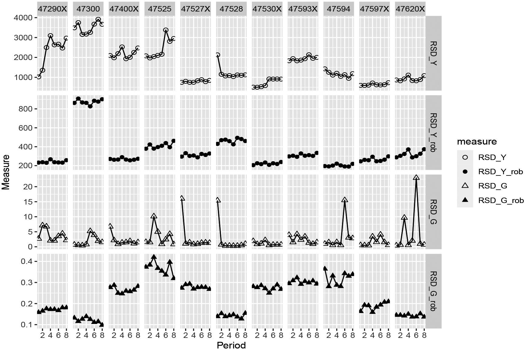
Similarly, we defined the RSD of a growth factor of period t to r of unit i in domain d as:

and ndt,r stands for the size of the union of units in domain d in the sample for period t and r. Since we were aware that the distribution of turnover tends to be very skewed and also that growth rates can have outliers, we defined a robust version of the RSD for the growth factor Gd⁢it,r which is given by:

where the mean of the growth factor Gd⁢it,r is replaced by its median and the robust standard deviation (Rousseeuw [12]) is given by

with γ= 1/0.6745, which is a correction factor such that in case of a normal distribution, in expectation, the robust standard deviation equals the (classical) standard deviation. The robust RSD for the turnover Yd⁢it is defined as in Eqs (8) and (9), but with Gd⁢it,r replaced by Yd⁢it. Cases in Eqs (3.4.2) and (8) where Yd⁢it=0 or Yd⁢ir=0 so that Gd⁢it,r is 0 or undefined, were treated separately. Furthermore, we tracked domains with many 0 values and verified the imputations that were based on them.

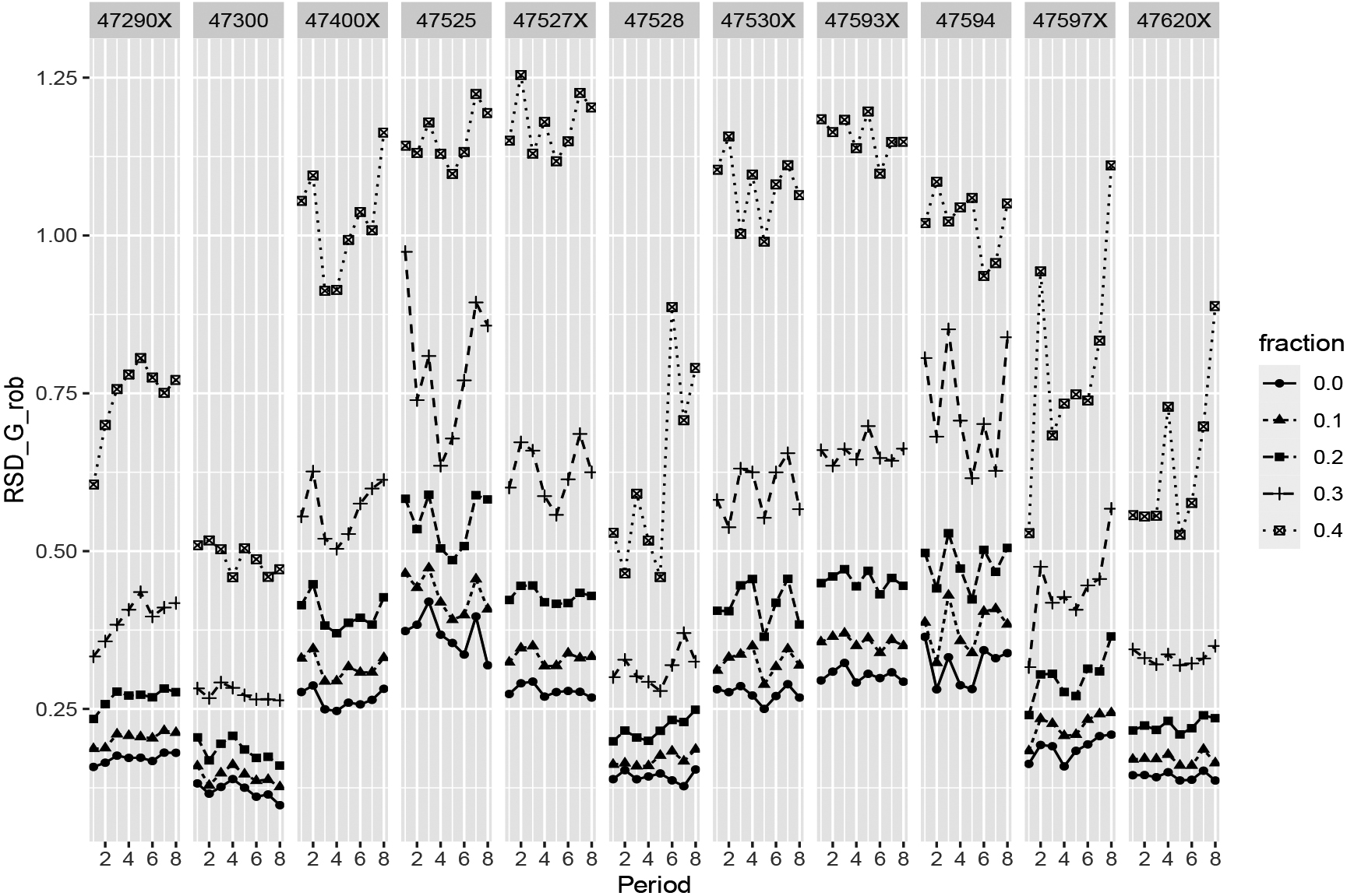
Figure 4.

Robust Relative Standard Deviation of the period-to-period growth factor as a function of the fraction of units with a very small growth factor, for eleven NACE codes in Retail trade from the first quarter of 2015 (period 1) till the forth quarter of 2016 (period 8). NACE codes are ending with ‘X’ when several underlying 5-digit codes are combined.

In order to verify whether it is reasonable to assume that the RSD per domain is constant over time but differs among domains, we computed the RSD⁢(Yd⁢it) and RSD⁢(Gd⁢it,t-4), and their robust version, for industries in Manufacturing, Retail trade and Employment services using historical VAT data of 2014–2016 for small and medium-sized enterprises on a quarterly basis. We only included records with turnover values larger than zero for both quarters of the year-on-year factor. As an example we plotted the results for some industries in Retail trade, see Fig. 3. We found that for some industries RSD⁢(Yd⁢it) and RSD⁢(Gd⁢it,t-4) varied considerably over time, especially RSD⁢(Gd⁢it,t-4). Their robust counterparts were more stable over time. For the imputations (see next section) often domains are used that are more detailed than the domains that we used in Fig. 3. We did some further analyses on these data and found that domains should have 30–40 units for the RSD(rob) to be stable over time.

We expected that in some domains the lockdown measures might have affected part of the units in a domain while other units were not or less affected. For instance because they were less dependent on a physical shop for their sales. In such conditions, it might well be that RSD⁢(Gd⁢it,r)⁢(rob) is increased compared to a pre-COVID-19 period. Since the growth factor of a domain, Gdt,r, is often used in the ratio imputation of the STS statistics, a larger spread of these growth factors may lead to imputations of a lower quality. To test whether a lockdown indeed increases the RSD⁢(Gd⁢it,r)⁢(rob), we computed the RSD⁢(Gd⁢it,r)⁢(rob) for the same industries and historical data as explained before, but this time we simulated that some of the units (randomly drawn) were affected by a lockdown. We tested fractions of 0.0, 0.1, 0.2, 0.3, 0.4, 0.45 and 0.5. For the affected units, we drew a growth factor at unit level (Yd⁢it/Yd⁢ir) from a normal distribution with mean 0.05 and standard deviation 0.0025 while the other units kept their original values. Results for the fraction up to 0.4 are shown in Fig. 4 for the same industries and periods as Fig. 3. The RSD⁢(Gd⁢it,r)⁢(rob) clearly increased with an increased proportion of units that is affected by the lockdown. However, at proportions larger than 0.4 (not shown for clarity of the figure), the RSD⁢(Gd⁢it,r)⁢(rob) dropped down to a small positive values due to the use of the absolute median difference. For some industries this drop occurred already earlier, because in the original data were also units with very small growth factors.

To support the production of the STS, we did not directly look at the RSD(rob) itself, but we computed the ratio Hdt,r,j (where H stands for heterogeneity measure) defined as:

where t stands for a period with lockdown measures, reference period r is either one period earlier or the same period one year earlier and t-j and r-j stand for pre-COVID-19 periods.

The ratio Hdt,r,j was used to support the production of the STS from the first lockdown period onwards. For the results over years 2018–2020 we took j to be one year (Dutch: jaar), so t-j and r-j are one year before periods t and r respectively. For 2021 we took j to be two years to ensure that t-j and r-j stand for pre-COVID-19 periods. Figure 5 shows the values of Hdt,t-12,j for year-on-year growth factors of monthly turnover for domains processed by the SSD system. We found an increased number of domains with Hdt,t-12,j> 2 in March-June 2020 and in January-May 2021, which concerned mainly domains in Retail trade (not shown). In these two periods there was a lockdown in which many shops were closed. From the beginning of April 2021 till end of June 2021 the lockdown measures were gradually released. In a very limited number of domains we found values of Hdt,t-12,j that were close to 0.

Figure 5.

For each month, the number of domains in the SSD system with the ratio Hdt,t-12,j larger than 2. The first plotted month is January 2018.

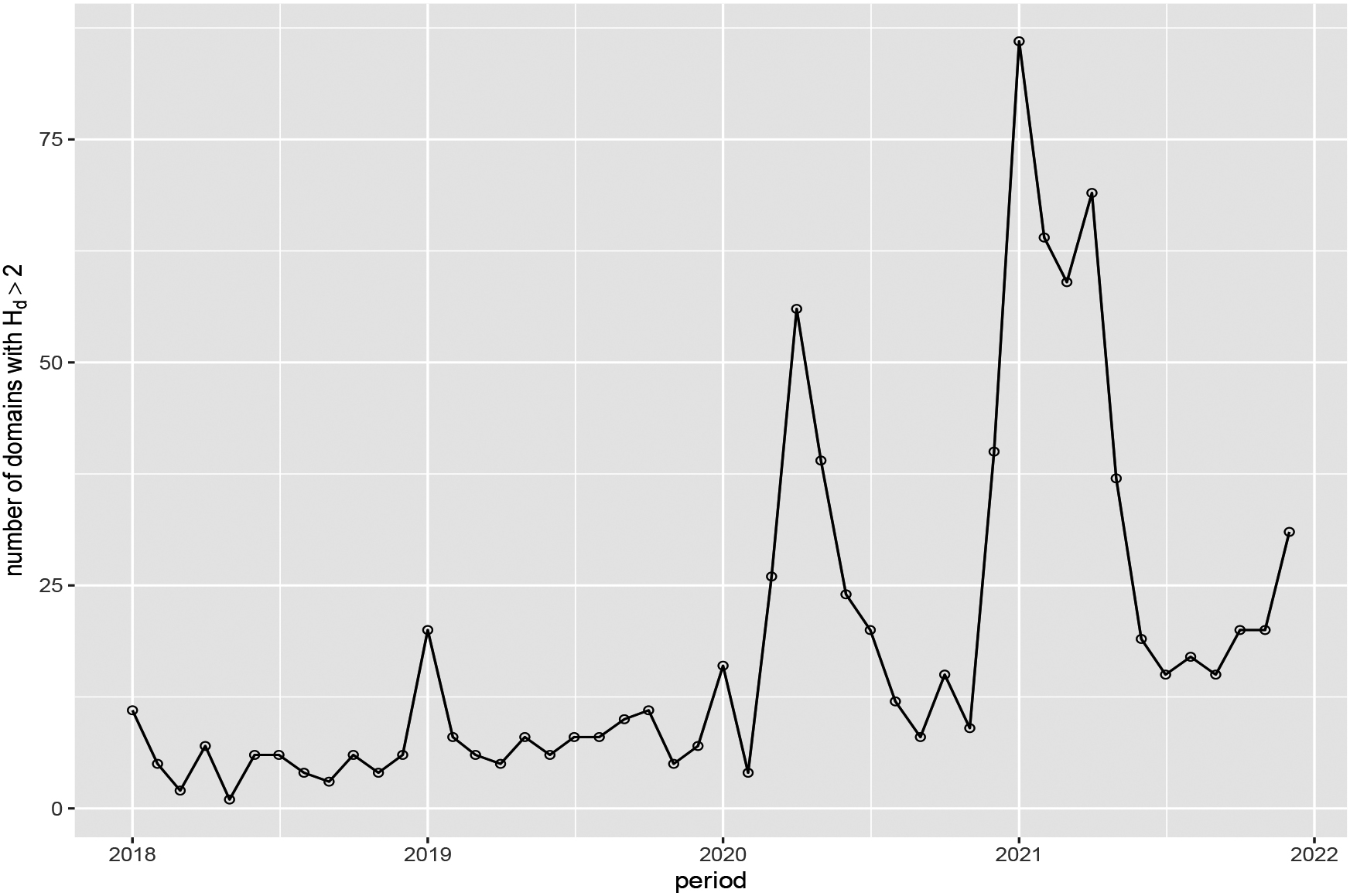
We aimed to compute a similar series of Hdt,t-4,j for year-on-year growth factors for quarterly turnover for domains in the CCD system, but we could not easily produce such a time series. Still, results for the second quarter of 2020 have been calculated and stored. In the second quarter of 2020 there were a large number of domains with Hdt,t-4,j> 2, for instance domains within NACE 5510 (Hotels and similar accommodation), 7912 (Tour operator activities) and 96021 (Hairdressing). We also found a considerable amount of domains where RSD (rob) dropped nearly to zero, also domains affected by the lockdown. This might be largely due to the aforementioned limitation of RSD (rob) in situations where a large proportion of the units in the domain has a turnover drop to almost zero.

For all domains with an increased heterogeneity, the imputed values were checked on plausibility. In case of the SSD system, for a few industries imputed values were adjusted. In case of the CCD system, first alternative imputations were computed for all domains, see Section 3.4.3, including domains with increased heterogeneity and domains where RSD (rob) dropped to small (positive) values. For a few industries the early estimates were adjusted, see also 3.4.3.

The heterogeneity score function has been a useful supportive means to check the quality of the imputations. Nonetheless, it would be good to try to improve the stability of this measure for smaller domain sizes since the domains that we use in practice often contain around 20 units. It would be good to test if using an α=1 makes RSD (rob) more stable at smaller domain sizes. Furthermore, preferably a measure of heterogeneity does not suddenly drop down to small values when fractions larger than 0.4 of the population become inactive.

3.4.3Alternative imputations: measures and results

Industries that were heavily affected by the lockdown measures and without high response rates during the early estimates, were mostly industries with quarterly statistics that are produced with the CCD system. During the production of the early quarterly estimates, used by National Accounts, many enterprises have not yet responded. Contributions of imputations to total turnover at industry level of more than 40% were no exception. We anticipated biased estimates due to an increased heterogeneity coupled with differential nonresponse within the industries. For example, if enterprises that were more affected by the lockdown responded earlier on average, then the early estimates would be biased downwards. Therefore, we took some measures for these quarterly statistics (CCD system). For the monthly statistics (SSD system) no further measures were needed, because the response rates turned out to be very high for the monthly industries that were affected by the lockdown measures, see Section 3.2.

As a potential measure to improve the imputations we analysed newly obtained auxiliary data, namely on enterprises applying for a COVID-19 subsidy (compensation for the wages of the employees). Those enterprises had to report an ‘expected turnover drop’ compared to the pre-COVID-19 situation. We analysed these new auxiliary data in relation to available turnover data for industries with monthly statistics. By the time that we received those data, two months of actual turnover data were already available. Since we intended to use the auxiliary data for the early estimates of the quarterly statistics, there was no time to perform a good analysis with actual turnover information for industries with quarterly estimates. However, the analysis with turnover data for industries with monthly statistics gave us confidence that the auxiliary data could be used in an imputation model also for the industries with quarterly statistics.

We made strata based on whether the enterprise applied for the subsidy and actually received a subsidy. The enterprises that actually received a subsidy were further stratified according to the expected turnover drop (20–30%, 30–40%, 40–60%, 60–100%), see Table 4. Based on the monthly survey data of all industries available in SSD for April and May, we computed separate year-on-year growth rates for each of those strata, see Table 4. The actual observed turnover drop as averaged over industries was found to be small for enterprises that did not receive a subsidy, whereas it increased with an increase of the reported expected turnover drop for the enterprises that did receive a subsidy.

We concluded that the new auxiliary data could be useful to improve the imputations for the early estimates of the quarterly industries in the CCD system (although the previous analysis was necessarily carried out for the monthly industries). We wrote a script to compute the same ratio imputation as in CCD (see Section 3.4.1, also with the same auxiliary information), but with the domains further subdivided according to strata based on the new auxiliary data. We computed four alternative imputations, both a simple stratification (presence/absence in application) and extended stratifications based on expected turnover drop categories. In a few cases no alternative imputations were calculated because the number of respondents was deemed too low (fewer than 10). Apart from these alternative imputations, the heterogeneity measures described in Section 3.4.2 were calculated as well.

In general, we found that the overall effect of the alternative imputations was limited. Depending on the exact method, the year-on-year growth rates with the alternative imputation method were 0.2–0.6 percentage points higher than with the normal imputation procedure (over all sectors with an early estimate from CCD). This indicated that early respondents on average had a lower turnover growth than late respondents within the original domains (without using the new auxiliary data). The effect was of the same order of magnitude as the known bias of the early CCD estimates in pre-COVID-19 periods, see also Section 3.5.1.

In Table 5 we give illustrative examples for some selected industries. The results for the four alternative imputations are given and the last column shows the final proposed values for our early CCD estimates (that are subsequently used as input by National Accounts). For most industries the effect of the alternative imputations was negligible, even for industries that were seriously affected by the lockdown measures like NACE code 55100 (‘Hotels and similar accommodation’) and 56101 (‘Restaurants’). For some industries a larger relative effect was found, but these often turned out to be small industries, like NACE code 58200 (‘Software publishing’). For a small number of larger industries, such as NACE code 63100 (‘Data processing, hosting and related activities; web portals’) and 71120 (‘Engineering activities and related technical consultancy’), a moderate effect was seen. But overall, the impact of the alternative imputations was small. One should keep in mind that the early estimates are not published at this detailed level. They are used as input for the early National Accounts estimates which are published at a much less detailed level. The alternative imputations for the CCD system were used to adjust the estimates of a few of the industries that were sent to National Accounts.

3.5.1Anticipated effects

The CCD system for the quarterly estimates uses ratio imputation to account for missing turnover values, see Section 3.4. Unfortunately, we know that the early estimates are typically slightly biased downwards. Therefore, for a few years alternative nowcast estimates have been used to support the regular analysis. The CCD estimates are still the basis for the early estimates used by National Accounts, but the analysts can adjust these estimates. The nowcast estimates use ARIMAX and VAR models with autoregressive terms and, as explanatory auxiliary variable, a time series based on the historical turnover of the enterprises with early response for the current period, as explained in Schouten [13].

We anticipated that, during the COVID-19 crisis, the nowcasting method with autoregressive terms might lead to a bias since – during periods of fast economic changes – time patterns in the past are no longer good predictors of the present.

3.5.2Measures

We advised the analysts not to use the quarterly nowcast estimates as a reference during the crisis, but only to use the early CCD estimates based on ratio imputation. The analysts have followed this advice and have not used the nowcast estimates as a reference ever since.

3.5.3Results

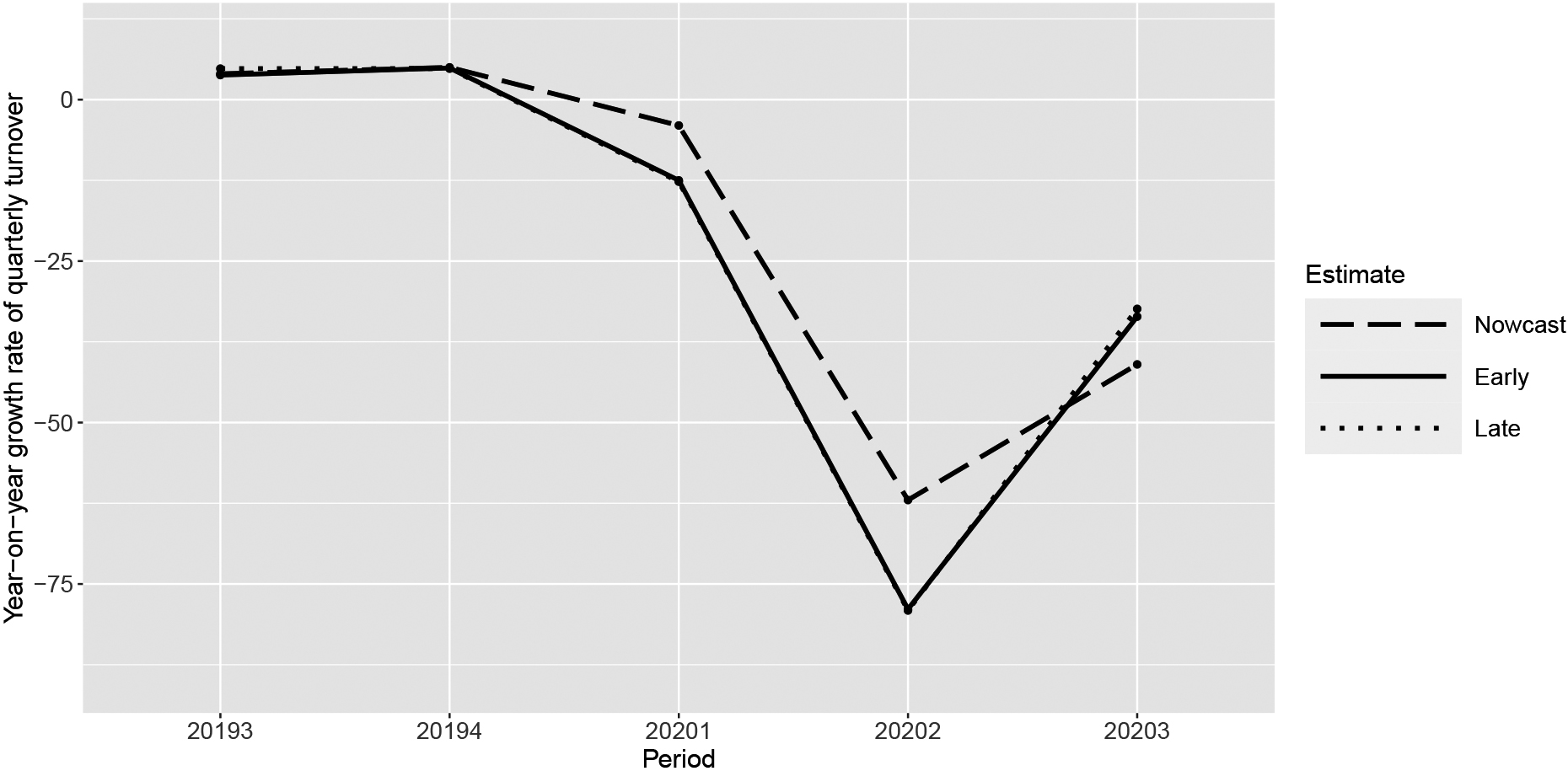
Figure 6 shows year-on-year growth rates (%) for the sector “Hotels and similar accommodation” for quarters just before the crisis and during the beginning of the crisis. The dotted line shows the late estimates when most enterprises have responded. These results are reliable and so early estimates close to the late estimates are considered to be good estimates. Both the early CCD estimates (solid line) and the quarterly nowcast estimates (long dashed line) are also shown in Fig. 6. For this industry a vector autoregression (VAR) model was used as the nowcast, see Schouten [13] for details on the model. In the VAR model dummy variables for the quarters are also included to account for seasonal effects.

In Fig. 6 a dramatic turnover drop of 79% is seen for the second quarter of 2020. The quarterly nowcast model also showed a large drop of 62%, but the estimate was 17 percentage points too high. The turnover drop started in the first quarter of 2020, which was expected since the first lockdown started mid-March 2020 in the Netherlands. For this quarter the nowcast year-on-year estimates were also far too high. Furthermore, the nowcast underestimated the partial recovery in the third quarter. The same pattern was observable for many other industries. At an aggregate level of all industries with quarterly turnover estimates in NACE sections I, J, M, N and S together, the turnover was estimated to drop by 19% in the second quarter according to the late CCD estimates and the early CCD estimates whereas the nowcast estimated a 11% drop. While the nowcast estimates were not accurate during the crisis, the regular early CCD estimates were rather accurate. The aforementioned bias in the early CCD estimates is of an order of magnitude of 0.5 percentage points, much smaller than the effects seen for the nowcast estimates during the economic downturn.

Figure 6.

Year-on-year growth rates of quarterly turnover of Hotels and similar accommodation, for the nowcast estimate, and early and late CCD estimates.

The bad performance of the quarterly nowcast estimates during the crisis is logical. Autoregression terms in ARIMAX and VAR tend to pick up sudden changes slowly. This might be desirable for early estimates during economically stable periods because a sudden change in turnover of a limited number of observed units might be due to noise. In case of a crisis however, sudden changes in observed turnover might be mainly caused by real economic changes and therefore should not be suppressed. Based on the reliable late estimates we concluded that the changes during the crisis were predominantly real and that the suppression of these changes was largely undesirable.

3.5.4Implications for the monthly nowcast

The findings with these kind of autoregressive models during this crisis also impacts another development, namely the new monthly figures that have to be produced by the Netherlands from 2024 for NACE sections G45, G46, H, I, J, L, M, N, see our explanation in Section 2. CBS has decided to estimate these monthly figures for all these sections, except for G46 and L, using a nowcasting model with monthly VAT data from most enterprises and monthly questionnaires for a small group of large enterprises as input. Since most businesses declare VAT on a quarterly basis in the Netherlands, the monthly input data is incomplete and selective. The monthly nowcast method aims to correct for that selectivity, based on quarterly information from the past, using autoregressive terms.

Because such a standard nowcasting approach may lead to biased estimates during a crisis, alternatives are investigated at CBS. This is work in progress. One idea is to incorporate imputed data in the nowcasting models, since the ratio imputations turned out to react quickly to sudden changes in growth rates which may occur when the economic conditions changes. It will be interesting to compare different imputation methods on their reaction to sudden economic changes. Another idea is to have a system that can accommodate two methods, the autoregressive nowcast model during “normal” periods and a method leaning heavier on recent response for periods with large economic changes. A critical question is how to determine when a crisis has started, see also the discussion in Smith and Lorenc [14]. In case of the COVID-19 crisis with accompanying lockdowns, this might be obvious but the situation might be more subtle for other crises. Furthermore, a crisis may not only affect the accuracy of nowcasts during a crisis, but due to its impact on model estimates (e.g. estimates of trends, seasonal patterns, autoregressive relations) it may also affect the accuracy of nowcasts after a crisis has passed. Therefore, a relevant question is also to ask, after a crisis, when to switch back to a nowcasting model that leans heavier on historical patterns. One could investigate this question by studying nowcasts using data of a real crisis that occurred in the past, which requires that such long microdata time series are available. To use the real data on the economic crisis of 2008, preferably microdata from about 2001 onwards should be available. Unfortunately it was not easy to construct such a microdata set due to changes in the IT systems used for the STS that occurred over the years. Instead, Zult et al. [15] have simulated three different crisis scenarios using the currently available microdata as a starting point and investigated their impact on different nowcast estimates.

3.6.1Anticipated effects

The estimated index of the target variables of the STS of industry k of the current period t (with base period 0), denoted by I^kt,0, is computed as a chained index, i.e. as the index of the previous period times a period-on-period growth factor:

with

and

where G^kt,t-1 stands for the estimated period-on-period growth factor of industry k. Throughout this paper a hat stands for an estimate. The weights dk⁢ix⁢(t,t-1) are based on the sampling design of periods t and t-1 and can be lowered in case of outliers; in case of the CCD system all weights dk⁢ix⁢(t,t-1) are 1. In case of the SSD system, nkx⁢(t,t-1) refers to units in the sample, in case of the CCD system it involves all units in the population. The symbol δk⁢ix⁢(t,t-1) indicates if unit i is included in the summation (δk⁢ix⁢(t,t-1)=1) or not (δk⁢ix⁢(t,t-1)=0). Sometimes units are excluded in situations of a restructuring. A restructuring concerns a merger, split and so on. In such a case, depending on certain conditions, either the unit is excluded for both periods (t,t-1) or the turnover is estimated for both periods (t,t-1) according to the same structure. Further, enterprises that change from industry are also excluded from both periods. For the various reasons just described, the turnover estimate of industry k for period t (denoted by Y^kt⁢(t,t-1)) that is used to calculate the growth factor G^kt,t-1 can differ from the turnover estimate for period t (denoted by Y^kt⁢(t+1,t)) for the subsequent growth factor. The estimates Y^kt⁢(t,t-1) and Y^kt-1⁢(t,t-1) are not intended to be accurate level estimates, the pair of estimates is used to estimate a period-on-period growth factor. Therefore, the index after a number of periods is not necessarily equal to the ratio of two directly estimated levels.

Due to an economic crisis, the accuracy of the index can be affected by a number of issues:

3.6.2Measures

As a first measure we did a number of specific analyses to address the issues a–f. These issues were analysed separately in the SSD and in the CCD system. Some of them were already part of the regular analysis, which is described in more detail in Section 3.8. In cases where an issue is expected to have a large impact on the results of an industry, we intended to do further analyses for that industry, for example by comparing results of the SSD system with those of the CCD system.

SSD and CCD were not equally sensitive to each of the mentioned potential problems. While SSD is sensitive to all the issues a–f, the CCD system is less sensitive to the issues b, c, d and f. Issue b is less relevant for CCD because its final estimates are based on census data; only the early estimates are based on an incomplete set of data, in which case heterogeneity may have an impact on the imputations, see Section 3.4. The CCD system is also less sensitive to c and f because it is not based on a sample but on a census. In general estimates based on census data encounter fewer estimation problems. Further, CCD is less sensitive to issue d because we expect that reporting errors on secondary activities mainly occur in survey data which is used for only a part of the target population.

As a second measure we intended to look into differences between the SSD and CCD results (for sections whose regular output is produced with the SSD system). This evaluation refers to different aggregation levels, to verify whether there are small effects within each industry that accumulate in the same direction. We intended to investigate these differences not only for total turnover but also for domestic and non-domestic turnover. Because issues a–f did not cause serious effects, see Section 3.6.3, we did not use this second measure.

A third measure was to verify for all industries whether the index returned to the correct level after the economy had normalised. This was done as follows. The first step was to detect whether there were any industries affected by the lockdown measures in which the index series might not have returned at their correct level: potentially incorrect series. This was done by computing trend lines in the seasonal adjustment software JDemetra+, by critically evaluating the plausibility of computed index series and – in case of industries produced by the SSD-system – by comparing their year-on-year changes with year-on-year changes of SSD-panel data. In the second step, we recomputed the indices of industries whose index series were detected as potentially incorrect. We recomputed the indices in different ways, making use of alternative index computations, which are described in detail in Van Delden and Van Bemmel [16]. An alternative index computation for Eq. (11) is given by:

where u is defined as a period before COVID-19 measures were taken, for instance January 2020, and t is the period of interest where the economy is (more or less) normalised. G^kt,u⁢(alt) stands for a growth factor between period t and u that is computed in an alternative way. A first alternative is:

where Y^kt⁢(L) denotes a level estimate for period t and industry k and Y^ku⁢(L) the corresponding level estimate for period u. In the CCD system such a level estimate can be approximated. However, for the SSD system, it requires quite some effort to make an accurate level estimate because the SSD system has not been designed for that purpose. The main purpose of the STS is to estimate a growth factor that is corrected for restructurings and for units with a change in industry. We therefore also defined a second alternative estimator for the growth factor:

This growth factor is computed similar to the computation of G^kt,t-1 in Eq. (12), but now for the periods t and u. In alt2 one uses pair-wise outliers and corrections for restructurings and for units that change from industry.

3.6.3Results

With respect to the first measure separate analyses were performed for the SSD system concerning the aforementioned issues a-f and for the CCD system for issues a and e, leading to the following findings:

In conclusion, the analysis of the specific issues indicated that most of the anticipated effects did not occur in practice. Still, we would do a similar analysis in a future economic downturn because it helped us to assure that the output was of a sufficient quality. Because no large effects were found for the SSD results, the second measure of comparing them with CCD results was not used.

With respect to the third measure, we did a preliminary check whether the index levels of affected industries in SSD and in CCD returned to their pre-COVID-19 levels by using trend lines in the seasonal adjustment software JDemetra+, in which the method X-13ARIMA-SEATS was used. Also, for SSD, year-on-year changes of the series were compared with year-on-year changes of panel data. These analyses did not yield any index series where adjustments were needed.

Next, validation of the times series up to Q3 2021 showed that the indices of NACE codes 79120, 59140, 55100 and 56300 had a very sharp drop during one or both of the lockdown periods and the indices might not have returned at the correct level after the measures were lifted. Therefore, indices were recomputed using different forms of Eq. (15) that varied in which set of two periods (t,u) was used. From that step it was concluded that only for NACE code 79120 (Tour operating agencies) a revision of the published data was necessary, for the other NACE codes differences between the alternative indices and their original ones were limited. For the revision of the NACE 79120 indices, we used Eq. (16) with t equal to Q3 2020 and u equal to Q1 2020. We used Eq. (16) because in the STS one aims to correct for the effects of restructurings. The original versus the recomputed index series for NACE code 79120 is given in Table 6. Especially at period Q3 2021 there was a large downwards correction of the original published index. Later, when the results for all quarters of 2021 were finalised, we computed final corrections.

3.7.1Anticipated effects

For the STS, index series are created which are calendar and seasonally adjusted. The first effects of the lockdown measures on the adjusted series were observed for the reporting period of March 2020. At that time, we anticipated the occurrence of a sharp decline or increase in the values of economic variables from March 2020 onwards. In crisis situations, the need for adjusted figures is even higher than normally because of the need to be able to separate the “crisis effect” from the calendar and seasonal effects. However, a crisis can destabilize the seasonal trends if extreme values are not accounted for in the (X-13 ARIMA-SEATS) models. In particular, the model estimates are very sensitive to the decision whether the most recent data points are deemed atypical or not. If crisis periods are not designated as outliers in the modelling, this could lead to unreliable figures and to substantive revisions for the already published figures (the whole series).

In seasonal adjustment, we consider four types of outliers:

See for more detailed information JDemetra+ [17] and United Nations [18].

Eurostat [19] gave advice with regard to calendar and seasonally adjusted figures, which also follows the ESS Guidelines (Eurostat [20]). Two potential outlier approaches were advised:

3.7.2Measures and results

For most industries that were affected by COVID-19, the first advised outlier approach of Eurostat (in Section 3.7.1) was used. During normal economic periods, the estimate of a period was detected as an outlier by using a Student t-test at a 1% significance level. The outlier detection at this threshold can be done automatically in the software JDemetra+. From the reporting month March 2020 onwards, the estimate of a period was detected as a potential outlier by using a Student t-test and by comparing its result with a 5% critical value of the Student’s t distribution, to be able to also appoint periods with less outlying values as outliers. A potential outlier was manually appointed to be a pre-specified, fixed, outlier in JDemetra+ when it was judged that the outlying effect was indeed due to the economic conditions. CBS made use of pre-specified outliers to ensure that the same periods are set as an outlier each time the time series is updated with new data. In contrast to the fixed, pre-specified, outliers, the periods that are automatically appointed as an outlier in JDemetra+ can change when the time series is updated.

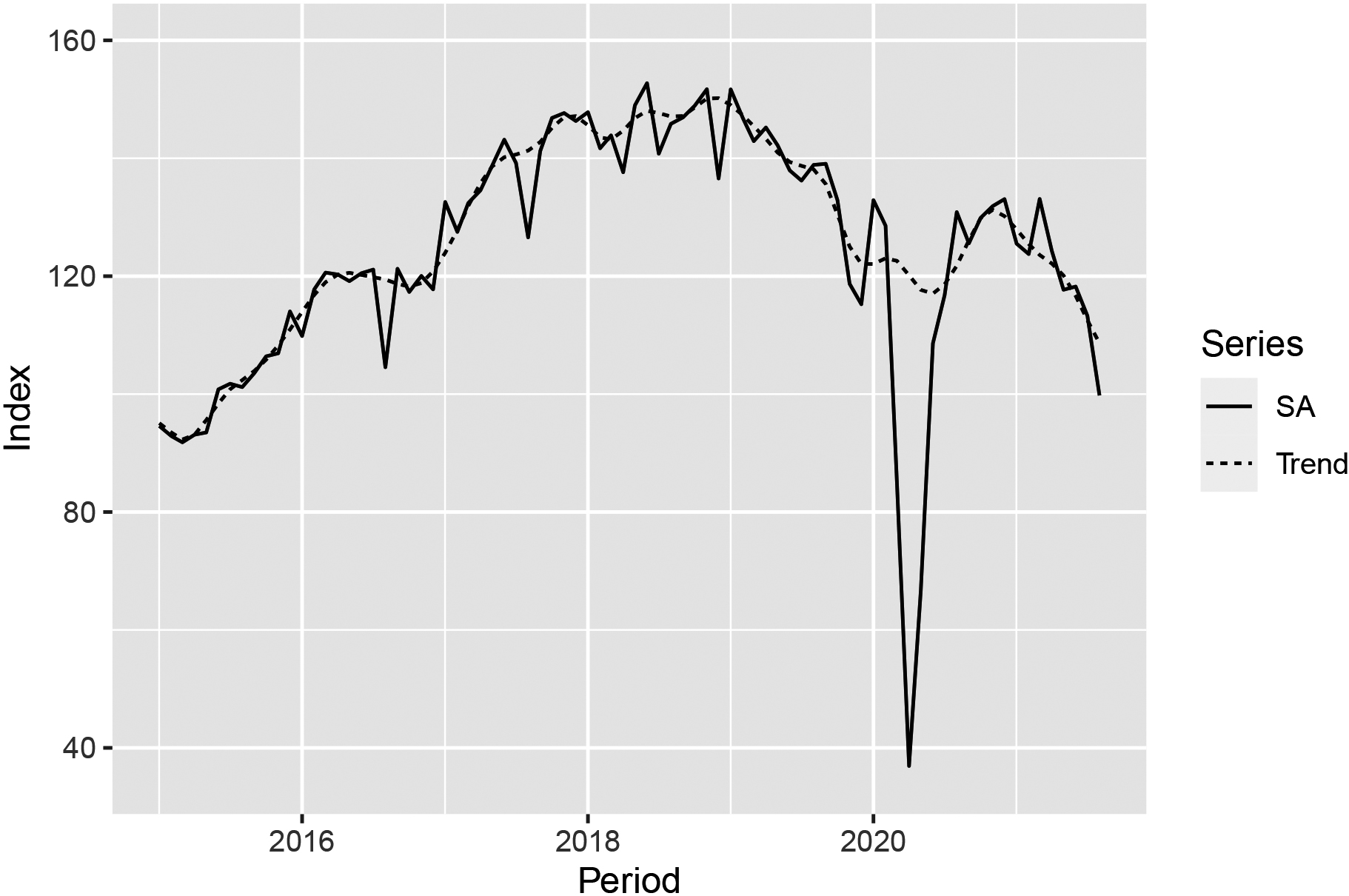
Figure 7.

Calendar and seasonally adjusted series (label: SA) of the volume of production and the trend line for NACE code 29 (Manufacture of motor vehicles and trailers).

One constantly monitored whether pre-specified outliers should be removed or added, whether other types of outliers were needed or whether one should define separate regressors (other auxiliary variables) within the seasonal adjustment to model the COVID-19 crisis. For series with too many appointed outliers (> 6 in 2020 for monthly figures and > 2 in 2020 for quarterly figures), the second advised outlier approach of Eurostat was used.

CBS put clarifications in the explanatory texts that is provided when publishing figures, to inform users about the outlier approaches and their effects. The approach where outliers are monitored “along the way” during an economic downturn enabled CBS to also take into account the seasonal effects for reporting periods that were less or not affected by COVID-19. Better estimations of the seasonal effects can be made years after the crisis has passed, see also the discussion in Section 4.

In Table 7 an illustration of this approach is given for the time series up to July 2020 for the index of the volume of production for the Manufacturing industries. The time series of volume of production represents the short-term volume changes of value added. For most industries CBS uses the deflated turnover to calculate these changes. For some industries CBS uses other information from big enterprises like working hours, produced quantities and orders. Table 7 shows that most outliers occurred in the second quarter of 2020 due to COVID-19 effects. Furthermore, some of the previously pre-specified outliers were dropped after the first analysis was done for the reporting month July 2020.

In Fig. 7 an example is given for the industry “Manufacture of motor vehicles and trailers” (NACE code 29). At the end of March 2020 and in April 2020, several influential manufacturers in the industry temporarily closed their enterprises and therefore we saw extreme production declines in these particular months. In May 2020 the volume index figures recovered. The pre-specified outliers for NACE code 29 are presented in Table 8. In the future, we will probably use a transitory change outlier because the index series has returned to a similar level as in the pre-COVID-19 situation. Without identifying the outliers in 2020, the values in March-May 2020 would have caused large revisions of the calendar and seasonally adjusted figures for reporting periods prior to 2020. Furthermore, it would also create problems for 2021. If the abnormal low values in 2020 had been accepted rather than set as pre-specified outliers, then the Students t-test for the months March, April and May 2021 would have been significant at a 5% threshold (see Table 9). Also, the trend for the previous and coming years would be somewhat affected if the outlying values in the second quarter of 2020 are not accounted for (see Fig. 8).

In the future we aim to determine if the additive outliers for all the impacted industries can be replaced by transitory change outliers or level shift outliers.

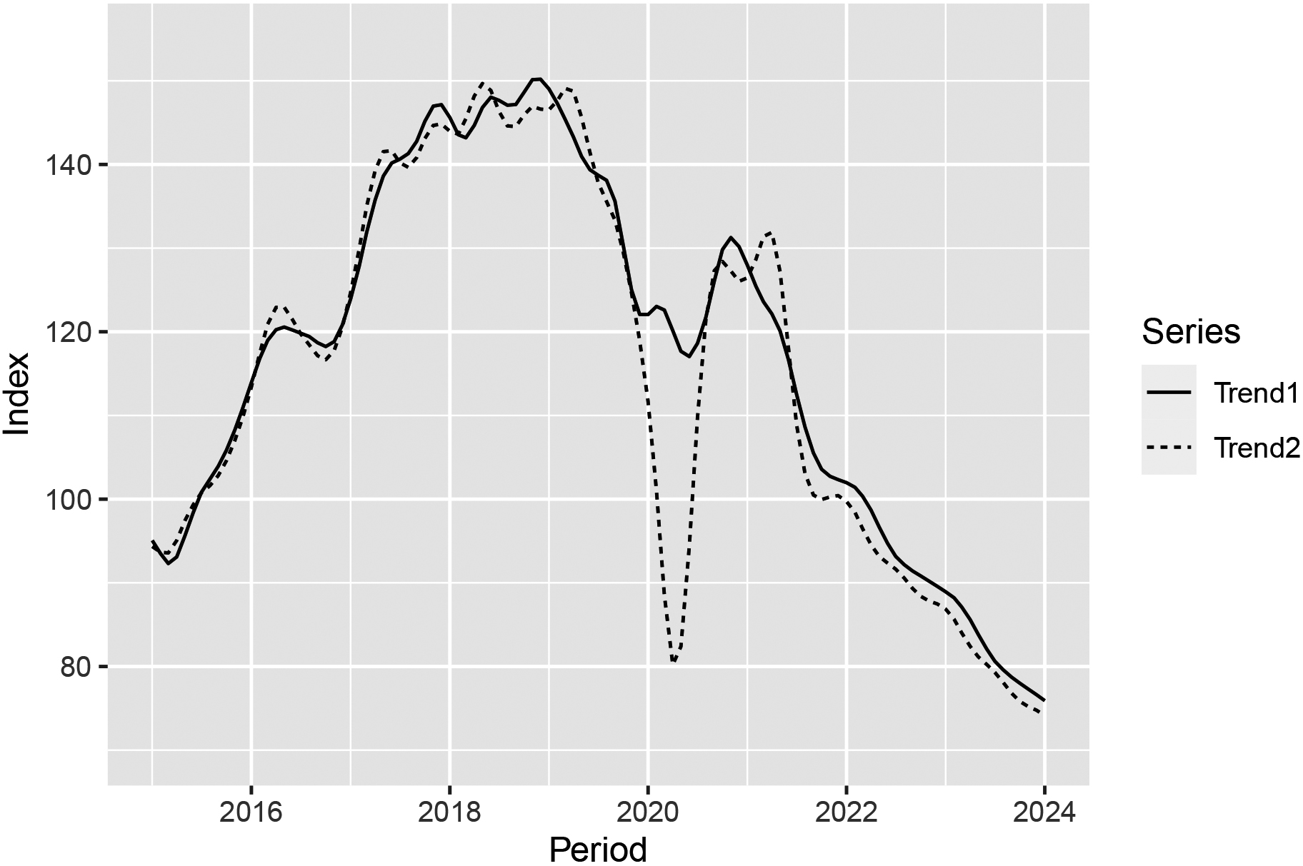
Figure 8.

The STS volume of production for NACE code 29 (Manufacture of motor vehicles and trailers), with two trend lines. For trend line 1 COVID-19 outliers are set for March, April and May 2020. Trend line 2 is without setting COVID-19 outliers for March, April and May 2020. The trend lines have been derived from the observed values from January 2000 up to and including August 2021 and predicted values from September 2021 up to and including August 2025. Results are shown up to the end of 2023.

One peculiarity we would like to mention is that the seasonal adjustment in our business cycle survey resulted in a value that was out of range. In this survey, one of the questions is whether respondents expect turnover in the coming three months to increase, decrease, or stay approximately the same. The estimated net effect yields a value between -100% (all entrepreneurs expect a turnover decrease) and 100% (all entrepreneurs expect a turnover increase). However, the calendar and seasonally adjusted figure for the hotel industry in Q2 2020 was estimated to be -112,6% due to an unadjusted value that was close to -100% combined with a negative (additive) seasonal adjustment term. CBS decided to suppress the seasonally adjusted figures for the hotel industry for Q2 2020.

References

[1] | RIVM; (2021) . Available from: https://www.rivm.nl/gedragsonderzoek/tijdlijn-maatregelen-covid. |
[2] | Brand M. Methodological Issues Arising for the Office for National Statistics from the Recession. In: European Establishment Statistics Workshop, 7–9 September 2009, Stockholm, Sweden; (2009) . Available from: https://statswiki.unece.org/display/ENBES/Topical+Papers. |
[3] | Simkins A, Smith PA, Brand M. Financial crisis and recession: How ONS has addressed the statistical and analytical challenges. Economic and Labour Market Review. (2010) ; 4: : 30–37. |
[4] | Eurostat. NACE Rev 2. Statistical classification of economic activities in the European Community. Eurostat Methodologies and Working papers. (2008) . |
[5] | Van Delden A, Scholtus S, Ostlund N. Modelling measurement errors to enable consistency between monthly and quarterly turnover growth rates. In: Proceedings of Statistics Canada Symposium 2018: Combine to Conquer: Innovations in the Use of Multiple Sources of Data; (2018) . |
[6] | Commission Implementing Regulation (EU) No 2020/1197 of 30 July 2020 laying down technical specifications and arrangements pursuant to Regulation (EU) 2019/2152 of the European Parliament and of the Council on European business statistics repealing 10 legal acts in the field of business statistics. Official Journal of the European Union. (2020) ; L 271: 1–170. |
[7] | Moreira A, Portugal A, Lima B, Poças J, Magalhães J, Cruz P, et al. The use of electronic invoice data in COVID time. In: European Establishment Statistics Workshop, 14–17 September 2021, online event; (2021) . |
[8] | Šuštar Kožuh L. Data collection in the light of COVID-19. In: European Establishment Statistics Workshop, 14–17 September 2021, online event; (2021) . |
[9] | Van Bemmel KJH, Goorden M. Imputation of turnover for short term statistics in case of extreme growth rates due to the COVID-19 crisis. CBS report (Available upon request, in Dutch). The Hague/Heerlen: Statistics Netherlands; (2020) . |
[10] | Van Delden A, Scholtus S. Analysing response differences between sample survey and VAT turnover. CBS Discussion paper. The Hague/Heerlen: Statistics Netherlands; (2019) . Available from: https://www.cbs.nl/en-gb/background/2019/22/analysing-response-differences-in-vat. |
[11] | Kutner MH, Nachtsheim CJ, Neter J, Li W. Applied Linear Statistical Models. Fifth edition ed. New York: McGraw-Hill Education; (2005) . |
[12] | Rousseeuw P. Least median of squares regression. Journal of the American Statistical Association. (1984) ; 79: : 871-880. |
[13] | Schouten B. Fast nowcasts with incomplete response. CBS report (Available upon request, in Dutch). The Hague/Heerlen: Statistics Netherlands; (2018) . |
[14] | Smith PA, Lorenc B. Robust official business statistics methodology during COVID-19-related and other economic downturns. Statistical Journal of the IAOS. (2021) ; 37: : 1079–1084. |
[15] | Zult D, Krieg S, Schouten B, Ouwehand P, Van Den Brakel J. From quarterly to monthly turnover figures using nowcasting. Journal of Official Statistics (conditionally accepted). (2022) . |
[16] | Van Delden A, Van Bemmel KJH. Indices as growth factors of the short term statistics in COVID-19 times. CBS report (Available upon request, in Dutch). The Hague/Heerlen: Statistics Netherlands; (2020) . |
[17] | JDemetra |
[18] | United Nations. Practical Guide to Seasonal Adjustment with Demetra |
[19] | Eurostat. Guidance on treatment of COVID-19-crisis effects on data. Luxembourg; (2020) . Available from: https://ec.europa.eu/eurostat/cros/system/files/treatment_of_covid19_in_seasonal_adjustment_methodological_note.pdf. |
[20] | Eurostat. ESS guidelines on seasonal adjustment. Luxembourg; (2015) . Available from: https://ec.europa.eu/eurostat/documents/3859598/6830795/KS-GQ-15-001-EN-N.pdf. |
[21] | CBS; (2022) . Available from: https://www.cbs.nl/nl-nl/visualisaties/welvaart-in-coronatijd. |
[22] | Zult D, Krieg S, Schouten B, Ouwehand P, Van Den Brakel J. From quarterly to monthly turnover figures using nowcasting. CBS Discussion paper. The Hague/Heerlen: Statistics Netherlands; (2020) . Available from: https://www.cbs.nl/nl-nl/achtergrond/2020/14/maandcijfers-over-omzet-met-behulp-van-nowcasten. |
[23] | CBS; (2022) . Available from: www.cbs.nl/coen. |
[24] | CBS; (2022) . Available from: https://www.cbs.nl/nl-nl/maatwerk/2021/27/gebruik-van-steunmaatregelen-corona-per-31-mei. |
[25] | Foley P. Seasonal adjustment of Irish official statistics during the current COVID-19 crisis. In: European Establishment Statistics Workshop, 14–17 September 2021, online event; (2021) . |
[26] | Olaeta H, Armendi J. Adapting seasonal adjustment procedures in uncertain times. In: European Establishment Statistics Workshop, 14–17 September 2021, online event; (2021) . |
[27] | Matthews S. Seasonal adjustment during the covid-19 pandemic: Statistics Canada’s approach. In: European Establishment Statistics Workshop, 14–17 September 2021, online event; (2021) . |
[28] | Jones J, McLaren C, Elliott D, Mead D, Baird H, Sakshaug J, et al. Producing Official Statistics during the COVID-19 Pandemic. Chapter 11 in: Snijkers G, Bavdaž M, Bender S, Jones J, MacFeely S, Sakshaug J, et al., eds. Advances in Business Statistics, Methods and Data Collection. John Wiley & Sons, Inc.; (2023) . |