A new generic method to improve machine learning applications in official statistics

Kloos, Kevin

doi:10.3233/SJI-210885

A new generic method to improve machine learning applications in official statistics

Article type: Research Article

Affiliations: Intern Methodologist, Statistics Netherlands (CBS), https://www.cbs.nl/en-gb/, The Hague, The Netherlands | E-mail: [email protected]

Correspondence: [*] Corresponding author: Intern Methodologist, Statistics Netherlands (CBS), https://www.cbs.nl/en-gb/, The Hague, The Netherlands. E-mail: [email protected].

Keywords: Misclassification bias, quantification, machine learning, official statistics, bias correction

DOI: 10.3233/SJI-210885

Journal: Statistical Journal of the IAOS, vol. 37, no. 4, pp. 1181-1196, 2021

Published: 26 November 2021

Get PDF

Abstract

The use of machine learning algorithms at national statistical institutes has increased significantly over the past few years. Applications range from new imputation schemes to new statistical output based entirely on machine learning. The results are promising, but recent studies have shown that the use of machine learning in official statistics always introduces a bias, known as misclassification bias. Misclassification bias does not occur in traditional applications of machine learning and therefore it has received little attention in the academic literature. In earlier work, we have collected existing methods that are able to correct misclassification bias. We have compared their statistical properties, including bias, variance and mean squared error. In this paper, we present a new generic method to correct misclassification bias for time series and we derive its statistical properties. Moreover, we show numerically that it has a lower mean squared error than the existing alternatives in a wide variety of settings. We believe that our new method may improve machine learning applications in official statistics and we aspire that our work will stimulate further methodological research in this area.

1.Introduction

National statistical institutes (NSIs) currently apply many different types of machine learning algorithms. Classification algorithms are one of the most popular types of algorithms because publishing aggregate statistics of (sub)groups in a population is one of the main tasks of national statistical institutes. Classical examples of classification algorithms are logistic regression and linear discriminant analysis, but also new innovative algorithms have been introduced over the last decades, like additive models, decision trees and deep learning [1]. Classification algorithms are optimized to minimize the summed loss of individual units, such that each unit has a high probability to be classified correctly. However, classifying units individually can lead to biased results when generalizing these individual units to aggregate statistics, like a proportion of the population [2, 3]. The cause of the biased results are imbalanced errors.

Before we show how generalizing units to aggregate statistics can lead to bias, we first emphasize the difference between a classifier and a quantifier. A classifier is a model that labels each unit to a class and a quantifier is a model that counts the number of units labelled to a class. Quantifiers can use classifiers in their model by counting the number of labels that the classifier has assigned to each class. Classifiers and quantifiers are imperfect because classification algorithms can mislabel some units. Each unit has a classification probability of being labelled correctly by the classification algorithm. A well-performing classifier has high classification probabilities for each labelled unit. A well-performing quantifier is not particularly defined by the number of mislabeled units, but by how the number of mislabeled units are distributed among the classes. In almost all cases, the number of mislabeled units among the classes don’t cancel each other out and as a consequence, bias will occur. The bias that occurs from imbalanced classification errors is called misclassification bias.

Misclassification bias cannot simply be solved by improving the accuracy of the classification algorithm. Moreover, a more accurate classifier can increase misclassification bias. For example, classifier A with 10 false positives and 10 false negatives is a worse classifier than classifier B with 9 false positives and 5 false negatives. However, when aggregating the results of both classifiers to a quantification, classifier A turns out to have less misclassification bias than classifier B and is, therefore, a better quantifier. Classifier A has less misclassification bias than classifier B because the number of mislabeled units in classifier A are equally distributed among both classes, while the number of mislabeled units in classifier B are unequally distributed among the classes. Therefore, improving a classifier is not the solution to reduce misclassification bias [3, 2].

We illustrate misclassification bias more extensively using an image-labelling example. The example shows us why using a standard approach for aggregating classifications from machine learning classifiers leads to problems. Suppose that a local government wants to estimate the number of houses in a certain area with solar panels on their rooftops. There is no register whether a house has a solar panel installation or not. It is an expensive and time-consuming task to manually label each rooftop, so the government decides to use satellite images combined with a classification algorithm to quickly label each house whether it has solar panels or not. Our target population consists of 10,000 houses, whereof 1,000 houses with solar panels and 9,000 without solar panels. Thus, the true proportion of houses with solar panels is 10%. The target variable is the proportion of houses with solar panels installation. Assume that the classifier can predict the rooftop images fairly accurate: 98% of the houses with solar panels are classified correctly (sensitivity) and 92% of the houses without solar panels are classified correctly (specificity). The machine learning algorithm classifies then 98% of the houses with solar panels and 8% of the houses without solar panels as houses with solar panels. This aggregates to 1,000×0.98+9,000×0.08=1,700 houses classified as a house with solar panels installation by the machine learning classifier. Thus, we estimate the proportion of houses with solar panels as 17% instead of the true value of 10%. The difference between the true proportion and the estimated proportion of houses with solar panels is called misclassification bias, and as the example demonstrates it can occur even when the classifier can predict every individual label with high accuracy.

Table 1

Confusion matrices of the target population and test set. Grey values are unknown in practice

True	Class 0	Class 1	Total
	Estimate
Class 0	N00	N01	N0+
Class 1	N10	N11	N1+
Total	N+0	N+1	N

True	Class 0	Class 1	Total
	Estimate
Class 0	n00	n01	n0+
Class 1	n10	n11	n1+
Total	n+0	n+1	n

(a) Target population

(b) Test set

In the literature, several corrections methods exist to reduce misclassification bias of the proportion of units labelled to the class of interest, i.e. the base rate. We compared statistical properties of the five most-used correction methods in a previous paper [4]. The correction methods contain information from the target population and a test set, see Table 1. The target population consists of N units that are labelled by a classification algorithm where we want to estimate the base rate from. The true labels are unknown in the target population, only the estimated labels are available. Therefore, the confusion matrix of the target population cannot be constructed in practice; only the column totals (white cells) in Table 1a are known. We construct a test set to get more information on the accuracy of the classifier. The test set consists of n≪N randomly sampled units from the target population that are both labelled by a classification algorithm and a human classifier. Therefore, we can construct a confusion matrix from the test set, see Table 1b, which contains information about the classification probabilities and the true base rate. In contrast to the target population, all the cells in the test set are known. The correction methods used in [4] exclusively contain information from the test set and the target population whereof closed-form equations of the mean square error (MSE) for each correction method could be computed. [4] concluded that the so-called calibration estimator works the best in general (more information in the next section).

However, the result from that paper does not generalize to time series. In other words, the results could not be applied for populations where the base rate changes over time. The target populations that are interesting for national statistical institutes, where we produce statistics on a monthly, quarterly or annual basis, change from period to period. The solar panel case is a good quantification example for time series: households can place solar panels on their roofs or displace them during a certain period. Moreover, the proportion of houses with solar panels is an interesting statistic concerning the government’s aims of renewable energy. The drift that occurs when the target population changes over time, is called concept drift [5]. In this paper, we assume a special case of concept drift called prior probability shift. Prior probability shift assumes that the base rate of a target population changes over time, but that the classification probabilities of units conditioned on their true label remain constant over time [6].

The most effective, but most costly and time-consuming solution to deal with prior probability shift, is to construct a new test set for each period. A more cost-efficient solution is to construct a test set and use the same test from period to period. As a consequence, we then cannot assume that a test set is a simple random sample of the target population when the base rate changes over time. Therefore, new expressions for bias and variance are needed to evaluate the MSE of the five correction methods. These expressions were previously computed by [7]. They concluded that none of those estimators performs consistently well under prior probability shift.

The main contribution of this paper is a new generic method to correct for misclassification bias when dealing with prior probability shift. We will refer to the resulting estimator as the mixed estimator because it combines the strengths of two existing estimators. We will derive (approximate) closed-form expressions for the bias and variance of the mixed estimator. Moreover, we will numerically compare the mixed estimator’s MSE with the classical methods.

The remainder of the paper is organized as follows: in Section 2, we introduce the problem and assumptions and we recap the properties of the original correction methods. Section 3 introduces the mixed estimator. Moreover, we will compare the mixed estimator with the original correction methods. Section 4 contains a discussion and conclusion of this paper.

2.Model under prior probability shift

In this section, we introduce the quantifier under prior probability shift. We use the same mathematical approach as in [4] and therefore use the same parameters and assumptions. Before we dive into the mathematical expressions, we briefly discuss the terminology used in the later sections. The target population has N units which belong to one of two classes, either class 0 or class 1. Our parameter of interest is the proportion of units that belong to class 1 in the target population, denoted as α. Similarly to [8], we assume that the underlying classifier has a probability of p00 to correctly classify an object of class 0 and a probability of p11 to correctly classify an object of class 1. These classification probabilities are unknown in practice, so we randomly sample a test set of size n from the target population. In the test set, both the true labels and the estimated labels are known. Then, we can make an estimate for p00 (p^00=n00n0+) and for p11 (p^11=n11n1+) with the test set. We assume that a binary classification algorithm has been trained that correctly classifies a data point that belongs to class i∈{0,1} with probability pi⁢i>0.5, independently across all data points. In addition, we assume that a test set of size n≪N is available and that it can be considered a simple random sample from the population. Finally, we assume that the classify-and-count estimator α^* is distributed independently of p^00 and p^11, which is reasonable (at least as an approximation) when n≪N.

In this paper, we allow that the base rate can change over time. In other words, we allow for a nonzero prior probability shift. Therefore, we introduce the following notation. First, we need to distinguish a target population U at time 0 from a target population U′ at time t. We can then define α′ as the base rate of the target population U′. Moreover, the classification probabilities of the target population are equal for U and U′, so the new base rate α′ is the only new parameter in this paper. Therefore, α denotes the base rate of target population U, whereof the test set is constructed.

Before we describe the differences between [4] and [7], we briefly introduce the correction methods. First, the baseline estimator (α^a) computes the proportion of units in the test set that belong to class 1. Second, the classify-and-count estimator (α^⋆) computes the proportion of units that are classified by the machine learning algorithm to class 1 in the target population. This is the naive estimator where we simply count the number of units that belong to class 1 according to the algorithm. Third, the subtracted-bias (α^b) estimator first estimates the bias of the classify-and-count estimator by estimating classification probabilities in the test set. Then, we compute the subtracted-bias estimator by subtracting this estimated bias from the classify-and-count estimator. Fourth, the misclassification estimator (α^p) multiplies the inverted row-normalised test set by the classify-and-count estimator. Last, the calibration estimator (α^c) multiplies the column-normalised test set by the classify-and-count estimator. An overview of the equations can be found in Table 2, as well as how these estimators perform in terms of bias and variance. The baseline, misclassification and calibration estimator are all (asymptotically) unbiased where the calibration estimator performs the best in general [7]. computed closed-form expressions of the bias and variance under prior probability shift. First, prior probability shift does not affect the mean square error of the classify-and-count estimator and subtracted-bias estimator majorly. The classify-and-count estimator does not use any information from the test set, so a different base rate does not affect this estimator. The subtracted-bias estimator only uses the test set to estimate the classification probabilities and therefore the estimator is not affected largely by the shift. Obviously, the baseline estimator cannot be used when the target population follows a different distribution than the test set. The misclassification estimator remains asymptotically unbiased, but the calibration estimator is unfortunately biased under prior probability shift. This is in contrast to the situation under a fixed base rate, where the calibration estimator is unbiased. Therefore, the misclassification estimator remains the only estimator that is (asymptotically) unbiased, see Table 3. According to [4] and [7], the misclassification estimator has a high variance when the classification probabilities are low. On the other hand, the variance of the misclassification estimator only changes slightly under prior probability shift. All in all, none of these correction methods have a consistently low MSE. In the next section, we will introduce a new estimator that performs better than the five original correction methods.

Table 2

Overview of the estimators without prior probability shift from [4]

Estimator	Equation	Bias	Variance
Baseline	α^a=n1+n	No	Large
Classify-and-count	α^⋆=N+1N	Large	Very low
Subtracted-bias	α^b=p^11⁢α^⋆+(1-p^00)⁢(1-Â⁢ ⁢α^⋆)	Medium	Low
Misclassification	α^p=α^⋆+p^00-1p^00+p^11-1	Very low	Large
Calibration	α^c=n10n+0⁢(1-Â⁢ ⁢α^⋆)+n11n+1⁢Â⁢ ⁢α^⋆	No	Medium

Table 3

Overview of the estimators under prior probability shift from [7]

Estimator	Equation	Bias	Variance
Baseline	α^a′=n1+n	Large	Large
Classify-and-count	(α^⋆)′=N+1′N	Large	Very low
Subtracted-bias	α^b′=p^11⁢(α^⋆)′+(1-p^00)⁢(1-(α^⋆)′)	Medium	Low
Misclassification	α^p′=(α^⋆)′+p^00-1p^00+p^11-1	Very low	Large
Calibration	α^c′=n10n+0⁢(1-(α^⋆)′)+n11n+1⁢(α^⋆)′	Medium	Medium

3.Mixed estimator

In this section, we introduce a new estimator: the mixed estimator. The mixed estimator is a combination between the misclassification estimator [9] and the calibration estimator [10]. In [4, 7], we found that the calibration estimator is unbiased under a fixed base rate, but becomes biased under prior probability shift. The misclassification estimator has a higher variance, but the MSE remains fairly stable under prior probability shift. These two properties can be combined: as an initial starting point, we take the calibration estimator α^c at time 0, but we add the difference between the misclassification estimator at time t(α^p′) and time 0 (α^p). Therefore, the expression for the mixed estimator is:

α^m′=α^c+[α^p′-α^p]

(1)

=n10n+0⁢(1-α^*)+n11n+1⁢α^*+(α^′)*-α^*p^00+p^11-1.

To the best of our knowledge, this is the first paper where the mixed estimator is introduced. Therefore, the closed-form expressions for bias and variance that we have derived are new as well.

.

The variance of the estimator p^11 for p11 estimated on the test set is given by

V⁢(p^11)=p11⁢(1-p11)n⁢α⁢[1+1-αn⁢α]+O⁢(1n3).

(2)

Similarly, the variance of p^00 is given by

(3)

V⁢(p^00)=p00⁢(1-p00)n⁢(1-α)⁢[1+αn⁢(1-α)]+O⁢(1n3).

Moreover, p^11 and p^00 are uncorrelated: C⁢(p^11,p^00)=0.

.

The mixed estimator α^m′ is a biased, but consistent, estimator for α′≠α:

(4)

B⁢[α^m′]=(α′-α)⁢(V⁢(p^00)+V⁢(p^11))(p00+p11-1)2+O⁢(1n2).

The variance of α^m′ is equal to:

V⁢(α^m′)

=α⁢p11n×(1-α⁢p11(1-α)⁢(1-p00)+α⁢p11)

+(1-α)⁢p00n×(1-(1-α)⁢p00(1-α)⁢p00+α⁢(1-p11))

+(α′-α)2×V⁢(p^00)+V⁢(p^11)(p00+p11-1)2+(α′-α)

×[α⁢p00⁢(1-p00)⁢(1-p11)+(1-α)⁢p00⁢p11⁢(1-p11)n⁢(p00-α⁢(p00+p11-1))⁢(p00+p11-1)

-α⁢p00⁢(1-p00)⁢p11+(1-α)⁢(1-p00)⁢p11⁢(1-p11)n⁢((1-α)⁢(1-p00)+α⁢p11)⁢(p00+p11-1)]

(5)

+O⁢(1n2).

Proof: See sec:appendix.

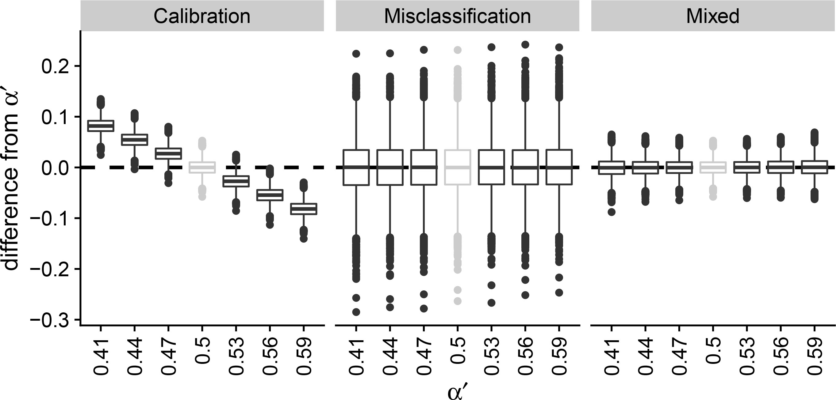
From Theorem 1, we see that the mixed estimator has a bias of O⁢(1n). Therefore, the mixed estimator is slightly biased but consistent. The variance function is complex, but we can see that the variance will be larger when the difference between α′ and α increases. To obtain a better overview of this mixed estimator, we will perform three simulation studies. Each simulation study consists of B=10,000 estimates for each correction method. First, we create fixed target populations given α,α′,p00,p11 and N: a population U at time 0 and a population U′ at time t. Then, we sample B=10,000 test sets of size n from population U and apply the estimators and equations from Table 3 on each test set.

In the first simulation study, we consider a class-balanced dataset (α=0.5), with a small test set of size n=1,000, a large population dataset of N=3×105 and a rather poor classifier having classification probabilities p00=0.6 and p11=0.7. From Fig. 1, we can see that the mixed estimator is in general a stable estimator with a low amount of bias and much less variance than the misclassification estimator. However, the variance of the mixed estimator tends to increase when the difference between α′ and α gets larger, which is in line with the observations in the previous paragraph. The mixed estimator performs much better than the misclassification estimator and the calibration estimator: it has almost no bias and has much less variance than the misclassification estimator.

Figure 1.

Simulation study to observe the change in prediction error under concept drift using boxplots. The calibration, misclassification and mixed estimator are compared given an initial base rate α=0.5 (grey) and different values of α′ (black). The test set is sampled from the target population with the initial base rate. The x-axis shows the different base rates and the y-axis shows the distribution of the difference from the new base rate α′. All the parameters: p00=0.6, p11=0.7, n=1,000 and N=3×105, B=10,000.

A situation where the mixed estimator does not work as well as expected, can be found in Fig. 2. We specify the following parameters: p00=0.94, p11=0.97, α=0.98, n=1,000, N=3×105 and B=10,000. The misclassification estimator tends to have more extreme outliers when the difference between α′ and α increases. This affects the mixed estimator in terms of variance. Furthermore, the mixed estimator can predict values outside the [0,1]-interval. We cannot encounter these values in practice and it is, therefore, a problem that we obtain these estimates. It seems that this problem occurs less often for the mixed estimator than for the misclassification estimator so the mixed estimator performs still better than the misclassification estimator and the calibration estimator individually. Finally, we can observe that the variance of the mixed estimator is always lower than the variance of the misclassification estimator. Despite the outliers, it is still the best estimator out of the three.

Figure 2.

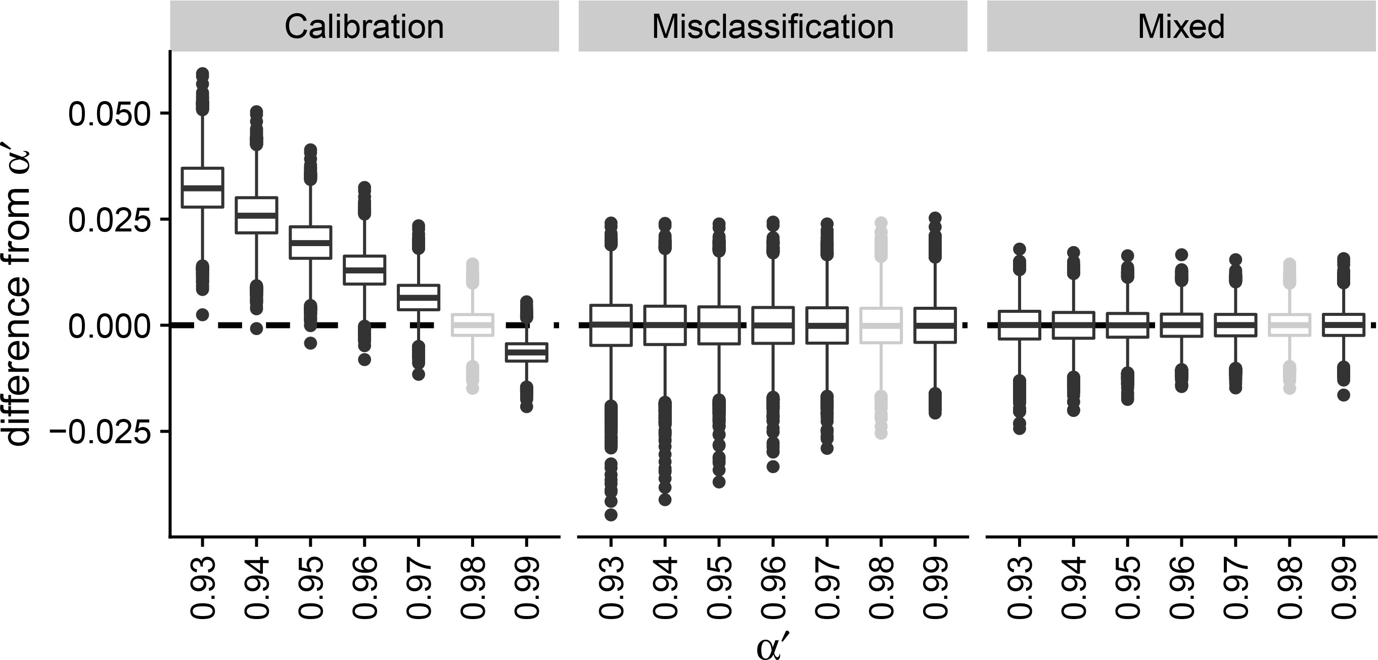
Simulation study to observe the change in prediction error under concept drift using boxplots. The calibration, misclassification and mixed estimator are compared given an initial base rate α=0.98 (grey) and different values of α′ (black). The test set is sampled from the target population with the initial base rate. The x-axis shows the different base rates and the y-axis shows the distribution of the difference from the new base rate α′. All the parameters: p00=0.94, p11=0.97, n=1,000N=3×105 and B=10,000.

Figure 3.

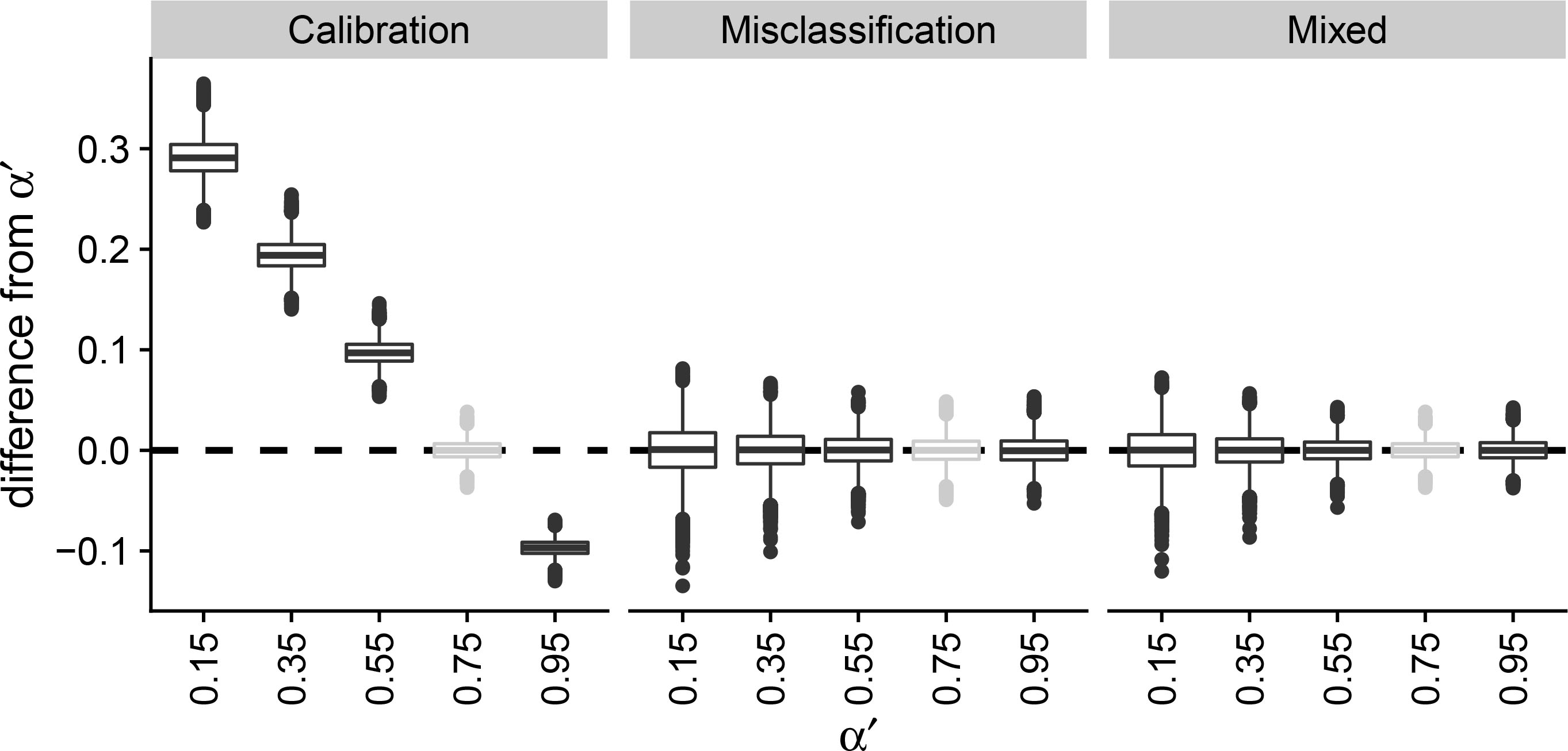
Simulation study to observe the change in prediction error under concept drift using boxplots. The calibration, misclassification and mixed estimator are compared given an initial base rate α=0.75 (grey) and different values of α′ (black). The test set is sampled from the target population with the initial base rate. The x-axis shows the different base rates and the y-axis shows the distribution of the difference from the new base rate α′. All the parameters: p00=0.85, p11=0.90, n=1,000, N=3×105 and B=10,000.

In the first two simulation studies, the misclassification estimator did not work properly, and we showed values of α′ that are close to α. It is also interesting to see what happens when the misclassification estimator has a low MSE for α and what happens when α′ differs substantially from α. We perform a simulation study with α=0.75, p00=0.85, p11=0.90, n=1,000, N=3×105 and B=10,000, shown in Fig. 3. We observe that the distribution of the mixed estimator is similar to the distribution of the misclassification estimator. The reason behind this is that the misclassification estimator performs similarly to the calibration estimator at time 0. However, the figures and the numbers show that the mixed estimator still performs consistently better than the misclassification estimator.

4.Conclusion and discussion

We conclude that our mixed estimator outperforms the estimators currently available in the academic literature. The mixed estimator has less bias than the calibration estimator and less variance than the calibration estimator. The mixed estimator performs much better than the calibration estimator and the misclassification estimator when the variance of the misclassification estimator is large but consistent over time. Our results show that the mixed estimator outperforms both the calibration estimator and the misclassification estimator in any dataset and for any classification algorithm used.

Even though that the new mixed estimator performs better than the original correction methods, we still believe that the correction methods might be improved further. We could construct a new estimator by combining biased, but invariant correction methods. New research directions lay in combining the correction methods in such a way that both bias and variance of the new estimator will be consistently low.

The estimator could be extended for correction methods that can predict more than two classes. The downside is that the number of parameters increases quadratically and the quality measure should be adapted for multiple classes. A possible solution is to further elaborate the simulation studies, instead of computing closed-form mathematical expressions. A final extension that we recommend is allowing the classification probabilities to differ between the units within a group, see [8].

With this paper, we hope that we raised awareness that aggregating outcomes of machine learning algorithms can be very inaccurate, even if the algorithms have a high prediction accuracy. Furthermore, this paper

is an addition to the scientific literature on the theory of misclassification bias. Finally, we proposed a new generic method that can be used by NSIs to improve machine learning applications within official statistics.

References

[1]	Friedman JH, Hastie T, Tibshirani R, et al. The elements of statistical learning. vol. 1. Springer, New York; (2001) .
[2]	Schwarz JE. The neglected problem of measurement error in categorical data. Sociological Methods & Research. (1985) .
[3]	Scholtus S, van Delden A. On the accuracy of estimators based on a binary classifier. (2020) ; 202006. Discussion Paper, Statistics Netherlands, The Hague.
[4]	Kloos K, Meertens QA, Scholtus S, Karch JD. Comparing correction methods to reduce misclassification bias. in: Artificial Intelligence and Machine Learning. Cham: Springer International Publishing; Baratchi M, Cao L, Kosters WA, Lijffijt J, van Rijn JN, Takes FW, eds, (2021) ; pp. 64-90.
[5]	Webb GI, Hyde R, Cao H, Nguyen HL, Petitjean F. Characterizing concept drift. Data Mining and Knowledge Discovery. (2016) ; 30: (4): 964-994.
[6]	Moreno-Torres JG, Raeder T, Alaiz-Rodríguez R, Chawla NV, Herrera F. A unifying view on dataset shift in classification. Pattern recognition. (2012) ; 45: (1): 521-530.
[7]	Meertens QA, Diks CGH, Van Den Herik HJ, Takes FW. Understanding the output quality of official statistics that are based on machine learning algorithms; (2021) .
[8]	van Delden A, Scholtus S, Burger J. Accuracy of mixed-source statistics as affected by classification errors. Journal of Official Statistics. (2016) ; 32: (3): 619-642.
[9]	Buonaccorsi JP. Measurement error: Models, methods, and applications. Boca Raton, FL: Chapman & Hall/CRC; (2010) .
[10]	Kuha J, Skinner CJ. Categorical data analysis and misclassification. in: Survey Measurement and Process Quality. Wiley; Lyberg LE, Biemer PP, Collins M, de Leeuw ED, Dippo C, Schwarz N, et al., eds, (1997) ; pp. 633-670.
[11]	Knottnerus P. Sample survey theory: Some pythagorean perspectives. Springer Science & Business Media; (2003) .

Appendices

Appendix

This appendix contains the proofs of the theorems presented in the paper entitled: A new generic method to improve machine learning applications in official statistics. Recall that we have assumed a population of size N in which a fraction α:=N1+/N belongs to the class of interest, referred to as the class labelled as 1. We assume that a binary classification algorithm has been trained that correctly classifies a data point that belongs to class i∈{0,1} with probability pi⁢i>0.5, independently across all data points. In addition, we assume that a test set of size n≪N is available and that it can be considered a simple random sample from the population. The classification probabilities p00 and p11 are estimated on that test set by row-normalizing the confusion matrix of the test set. Finally, we assume that the classify-and-count estimator α^* is distributed independently of p^00 and p^11, which is reasonable (at least as an approximation) when n≪N.

It may be noted that the estimated probabilities p^11 and p^00 cannot be computed if n1+=0 or n0+=0. Similarly, the calibration probabilities c11 and c00 cannot be estimated if n+1=0 or n+0=0. We assume here that these events occur with negligible probability. This will be true when n is sufficiently large so that n⁢α≫1 and n⁢(1-α)≫1.

Preliminaries

Many of the proofs presented in this appendix rely on the following two mathematical results. First, we will use univariate and bivariate Taylor series to approximate the expectation of non-linear functions of random variables. That is, to estimate E⁢[f⁢(X)] and E⁢[g⁢(X,Y)] for sufficiently differentiable functions f and g, we will insert the Taylor series for f and g at x0=E⁢[X] and y0=E⁢[Y] up to terms of order 2 and utilize the linearity of the expectation. Second, we will use the following conditional variance decomposition for the variance of a random variable X:

(6)

V(X)=E[V(X|Y)]+V(E[X|Y]).

The conditional variance decomposition follows from the tower property of conditional expectations [11]. Before we prove the theorems presented in the paper, we begin by proving Lemma 1.

Proof of Lemma 1 We approximate the variance of p^00 using the conditional variance decomposition and a second-order Taylor series, as follows:

V(p^00)=V(n00n0+)=En0+[V(n00n0+|n0+)]+Vn0+[E(n00n0+|n0+)]=En0+[1n0+2V(n00|n0+)]+Vn0+[1n0+E(n00|n0+)]=En0+[n0+⁢p00⁢(1-p00)n0+2]+Vn0+[n0+⁢p00n0+]=En0+[1n0+]p00(1-p00)=[1E⁢[n0+]+122E⁢[n0+]3×V[n0+]]p00(1-p00)+O(1n3)=p00⁢(1-p00)E⁢[n0+][1+V⁢[n0+]E⁢[n0+]2]+O(1n3)=p00⁢(1-p00)n⁢(1-α)[1+αn⁢(1-α)]+O(1n3).

The variance of p^11 is approximated in the exact same way.

Finally, to evaluate C⁢(p^11,p^00) we use the analogue of Eq. (6) for covariances:

The second term is zero as before. The first term also vanishes because, conditional on the row totals n1+ and n0+, the counts n11 and n00 follow independent binomial distributions, so C(n11,n00|n1+,n0+)=0.

Note: in the remainder of this appendix, we will not add explicit subscripts to expectations and variances when their meaning is unambiguous.

Mixed estimator

In this section, we will prove the bias and the variance of the mixed estimator under concept drift. The mixed estimator is dependent on the calibration estimator at time 0, the misclassification estimator on time 0 and the misclassification estimator on time t.

Proof of Theorem 1 First, we will make a proof for the bias of the Mixed Estimator. The expression for the Mixed Estimator is:

(7)

α^m′=α^c+(α^p′-α^p)=α^c+[(α^′)*-α^*]×1p^00+p^11-1.

The bias is defined as the difference between the expected value of the estimator minus the true value of the target variable:

(8)

B⁢[α^m′]=E⁢[α^m′]-α′

Using Eq. (7), we can write out the expected value of the mixed estimator.

(9)

E⁢[α^m′]=E⁢[α^c+[(α^′)*-α^*]×1p^00+p^11-1]=E⁢[α^c]+E⁢[[(α^′)*-α^*]×1p^00+p^11-1]

From [4], we already know that:

(10)

E[α^c]=E[α^c|α^*]=α.

E⁢[[(α^′)*-α^*]×1p^00+p^11-1] can be computed by conditioning on the Classify-and-count estimators (α^′)* and α^*.

(11)

E[[(α^′)*-α^*]×1p^00+p^11-1]=E[E[[(α^′)*-α^*]×1p^00+p^11-1|(α^′)*,α^*]]=E[((α^′)*-α^*)×E[1p^00+p^11-1|(α^′)*,α^*]]=E[((α^′)*-α^*)×E[1p^00+p^11-1]]

From [4], we used Taylor Series to approximate the expected value of 1p^00+p^11-1.

(12)

E⁢[1p^00+p^11-1]=1p00+p11-1+V(p^00)+Vp^11)(p00+p11-1)3+O⁢(n-2)

Now it only remains to calculate the expected values of the classify-and-count estimators.

(13)

E⁢[(α^′)*-α^*]=E⁢[(α^′)*]-E⁢[α^*]

(14)

E⁢[(α^′)*]=α′⁢p11+(1-α′)⁢(1-p00)=α′⁢(p00+p11-1)+(1-p00)

(15)

E⁢[α^*]=α⁢p11+(1-α)⁢(1-p00)=α⁢(p00+p11-1)+(1-p00)

Combining these expressions, E⁢[(α^′)*-α^*] can be simplified towards the following expression.

(16)

E⁢[(α^′)*-α^*]=(α′-α)⁢(p00+p11-1)

Combining Eqs (12) and (16) gives the expression that should be in the big expectation of Eq. (11).

(17)

E⁢[(α^′)*-α^*p^00+p^11-1]=E⁢[((α^′)*-α^*)×E⁢[1p^00+p^11-1]]=E⁢[(α^′)*-α^*]×E⁢[1p^00+p^11-1]=(α′-α)⁢(p00+p11-1)×[1p00+p11-1+V⁢(p^00)+V⁢(p^11)(p00+p11-1)3]+O⁢(n-2)=α′-α+(α′-α)⁢(V⁢(p^00)+V⁢(p^11))(p00+p11-1)2+O⁢(n-2)

Finalizing the proof given Eqs (8), (10) and (17).

(18)

B⁢[α^m′]=E⁢[α^m′]-α′=α+α′-α+(α′-α)⁢(V⁢(p^00)+V⁢(p^11))(p00+p11-1)2-α′+O⁢(n-2)=(α′-α)⁢(V⁢(p^00)+V⁢(p^11))(p00+p11-1)2+O⁢(n-2)

Now it only remains to prove the variance of the mixed estimator. Recall that the mixed estimator can be written as

(19)

α^m′=α^c+[(α^′)*-α^*]×1p^00+p^11-1.

It clearly follows from Eq. (19) that the variance of this mixed estimator can be written as

(20)

V⁢[αm′]=V⁢[α^c]+V⁢[(α^′)*-α^*p^00+p^11-1]+2⁢C⁢[α^c,(α^′)*-α^*p^00+p^11-1].

From [4], we already know that the variance of the calibration estimator is equal to

(21)

V⁢(α^c)=[(1-α)⁢(1-p00)+α⁢p11n+(1-α)⁢p00+α⁢(1-p11)n2]×[α⁢p11(1-α)⁢(1-p00)+α⁢p11⁢(1-α⁢p11(1-α)⁢(1-p00)+α⁢p11)]+[(1-α)⁢p00+α⁢(1-p11)n+(1-α)⁢(1-p00)+α⁢p11n2]×[(1-α)⁢p00(1-α)⁢p00+α⁢(1-p11)⁢(1-(1-α)⁢p00(1-α)⁢p00+α⁢(1-p11))]+O⁢(max⁡[1n3,1N⁢n]).

The second term in Eq. (20) makes use of previous assumptions in this paper. We can say that p^00 and p^11 are independent of our Classify-and-count estimators α^* and (α^′)*. Furthermore, a well-known result on variances states that for two independent random variables A and B, it holds that V⁢(A⁢B)=E⁢[A]2⁢V⁢(B)+E⁢[B]2⁢V⁢(A)+V⁢(A)⁢V⁢(B). Combining these statements gives

(22)

V⁢[(α^′)*-α^*p^00+p^11-1]=[E⁢((α^′)*-α^*)]2⁢V⁢[1p^00+p^11-1]+[E⁢(1p^00+p^11-1)]2⁢V⁢[(α^′)*-α^*]+V⁢[(α^′)*-α^*]⁢V⁢[1p^00+p^11-1].

Assuming that N≫n, we can make the statement that V⁢[(α^′)*-α^*] is of O⁢(1N).

(23)

V⁢[(α^′)*-α^*p^00+p^11-1]=[E⁢((α^′)*-α^*)]2⁢V⁢[1p^00+p^11-1]+O⁢(1N)

The expected value of the differences between the classify-and-count estimators is already computed in Eq. (16) and the variance term in Eq. (23) is already proven in [4]. This eases the derivation of the second term in Eq. (20).

(24)

V⁢[(α^′)*-α^*p^00+p^11-1]=(α′-α)2×V⁢(p^00)+V⁢(p^11)(p00+p11-1)2+O⁢(max⁡[1N,1n2])

Thus it remains to evaluate the covariance term in Eq. (20). By conditioning on the classify-and-count estimators α^* and (α^′)*, we obtain:

(25)

C[α^c,(α^′)*-α^*p^00+p^11-1]=E[C[α^c,(α^′)*-α^*p^00+p^11-1|(α^′)*,α^*]]+C[E[α^c|(α^′)*,α^*],E[(α^′)*-α^*p^00+p^11-1|(α^′)*,α^*]]

It can be proven that the second term of Eq. (25) is equal to zero. In Eq/ 10, we see that the expectation of the calibration estimator, given classify-and-count estimators, is equal to α. This is a constant and the covariance with a constant is equal to zero. Therefore, the covariance term can also be written as:

(26)

C[α^c,(α^⋆)′-α^*p^00+p^11-1]=E[C[α^c,(α^⋆)′-α^*p^00+p^11-1|(α^⋆)′,α^*]].

We can derive an expression for the inner covariance, which is written as

(27)

C[α^c,(α^⋆)′-α^*p^00+p^11-1|(α^⋆)′,α^*]=[(α^⋆)′-α^*]C[α^c,1p^00+p^11-1|α^*].

The terms in Eq. (27) can be written in terms of the test set (n00,n01,n10,n11). This eases the computation further on. Note that the elements of this test set do not depend on the classify-and-count estimator α^*.

(28)

C[α^c,1p^00+p^11-1|α^*]=C[n10n+0(1-α^*)+n11n+1α^*,1n00n0++n11n1+-1|α^*]=C[n10n+0(1-α^*)+n11n+1α^*,n0+⁢n1+n00⁢n11-n01⁢n10|α^*]=(1-α^*)C[n10n+0,n0+⁢n1+n00⁢n11-n01⁢n10]+α^*C[n11n+1,n0+⁢n1+n00⁢n11-n01⁢n10]

We are able to evaluate both covariance terms with the same methods. We can condition on one of the row totals. Note that the other row total is also fixed, because we work with binary classifiers (n1+=n-n0+). Furthermore, we are able to write as many variables as possible in terms of n0+ and n1+. This helps with the Taylor Series that we apply to approximate the covariances.

C⁢[n10n+0,n0+⁢n1+n00⁢n11-n01⁢n10]

=E[C[n10n+0,n0+⁢n1+n00⁢n11-n01⁢n10|n1+]]+C[E[n10n+0|n1+],E[n0+⁢n1+n00⁢n11-n01⁢n10|n1+]]

=E[C[n1+-n11n1++n00-n11,n0+⁢n1+n0+⁢n11+n1+⁢n00-n0+⁢n1+|n1+]]

(29)

+C[E[n1+-n11n1++n00-n11|n1+],E[n0+⁢n1+n0+⁢n11+n1+⁢n00-n0+⁢n1+|n1+]]

While we condition on the row totals, the other variables in the covariance functions are n00 and n11. Say

n10n+0=f⁢(n00,n11)⁢and⁢n0+⁢n1+n00⁢n11-n01⁢n10=g⁢(n00,n11),

with

(30)

f⁢(x,y)=n1+-yn1++x-y

(31)

g⁢(x,y)=n0+⁢n1+n1+⁢x+n0+⁢y-n0+⁢n1+

we are able to compute first-order Taylor series approximations for these terms to obtain an approximation for C⁢[n10n+0,n0+⁢n1+n00⁢n11-n01⁢n10].

(32)

∂⁡f∂⁡x=(n1++x-y)⋅0-(n1+-y)⋅1(n1++x-y)2=y-n1+(n1++x-y)2

(33)

∂⁡f∂⁡y=(n1++x-y)⋅-1-(n1+-y)⋅-1(n1++x-y)2=-x(n1++x-y)2

(34)

∂⁡g∂⁡x=-(n0+⁢n1+)⁢n1+(n0+⁢y+n1+⁢x-n0+⁢n1+)2=-n1+2⁢n0+(n0+⁢y+n1+⁢x-n0+⁢n1+)2

(35)

∂⁡g∂⁡y=-(n0+⁢n1+)⁢n0+(n0+⁢y+n1+⁢x-n0+⁢n1+)2=-n0+2⁢n1+(n0+⁢y+n1+⁢x-n0+⁢n1+)2

The approximation can be made with substituting x=E[n00|n1+] and y=E[n11|n1+] and applying the approximation rules for covariance. Given that n00 and n11 are independent from each other given the row totals, we can cross out C⁢(n00,n11).

(36)

In order to use this approximation, we can use the following properties:

E(n00|n1+)=n0+p00

V(n00|n1+)=n0+p00(1-p00)

E(n11|n1+)=n1+p11

V(n11|n1+)=n1+p11(1-p11)

Substituting these elements gives

(37)

C[n10n+0,n0+⁢n1+n00⁢n11-n01⁢n10|n1+]≈(n1+⁢p11)-n1+(n1++n0+⁢p00-n1+⁢p11)2×-n1+2⁢n0+(n0+⁢(n1+⁢p11)+n1+⁢(n0+⁢p00)-n0+⁢n1+)2n0+p00(1-p00)+-n0+⁢p00(n1++n0+⁢p00-n1+⁢p11)2×-n0+2⁢n1+(n0+⁢(n1+⁢p11)+n1+⁢(n0+⁢p00)-n0+⁢n1+)2n1+p11(1-p11).

This expression simplifies to

(38)

C[n10n+0,n0+⁢n1+n00⁢n11-n01⁢n10|n1+]≈n1+⁢p00⁢(1-p00)⁢(1-p11)+n0+⁢p00⁢p11⁢(1-p11)(n1++n0+⁢p00-n1+⁢p11)2⁢(p00+p11-1)2

Now that the inner covariance of Eq. (29) is computed, we can move on and calculate the inner expectations of Eq. (29). This can be done with a second-order Taylor series approximation.

(39)

∂2⁡f∂⁡x2=2×n1+-y(n1++x-y)3

(40)

∂2⁡f∂⁡y2=2×-x(n1++x-y)3

(41)

∂2⁡g∂⁡x2=2×n1+3⁢n0+(n0+⁢y+n1+⁢x-n0+⁢n1+)3

(42)

∂2⁡g∂⁡y2=2×n0+3⁢n1+(n0+⁢y+n1+⁢x-n0+⁢n1+)3

Applying the Taylor rules for approximating an expected value and substituting x=E[n00|n1+] and y=E[n11|n1+] into the equations gives:

(44)

E[n10n+0|n1+]≈n1+-E[n11|n1+]n1++E[n00|n1+]-E[n11|n1+]+n1+-E[n11|n1+](n1++E[n00|n1+]-E[n11|n1+])3V[n00|n1+]-E[n00|n1+](n1++E[n00|n1+]-E[n11|n1+])3V[n11|n1+]=n1+-n1+⁢p11n1++n0+⁢p00-n1+⁢p11+n1+-n1+⁢p11(n1++n0+⁢p00-n1+⁢p11)3n0+p00(1-p00)-n0+⁢p00(n1++n0+⁢p00-n1+⁢p11)3n1+p11(1-p11)

(45)

=n1+⁢(1-p11)n1++n0+⁢p00-n1+⁢p11+n0+⁢n1+⁢p00⁢(p11-1)⁢(p00+p11-1)(n1++n0+⁢p00-n1+⁢p11)3

(47)

(48)

=1p00+p11-1+n1+⁢p00⁢(1-p00)+n0+⁢p11⁢(1-p11)(n0+⁢n1+)⁢(p00+p11-1)3

The next step is computing the outer expectation and the outer covariance of Eq. (29). The outer expectation can be approximated with a zero-order Taylor series.

(49)

E[C[n10n+0,n0+⁢n1+n00⁢n11-n01⁢n10|n1+]]≈n⁢α⁢p00⁢(1-p00)⁢(1-p11)+n⁢(1-α)⁢p00⁢p11⁢(1-p11)(n⁢α+n⁢(1-α)⁢p00-n⁢α⁢p11)2⁢(p00+p11-1)2=α⁢p00⁢(1-p00)⁢(1-p11)+(1-α)⁢p00⁢p11⁢(1-p11)n⁢(p00-α⁢(p00+p11-1))2⁢(p00+p11-1)2

Furthermore, it can be proven that the outer covariance of the two expectations is of O⁢(1n2) and can therefore be neglected in Eq. (29). In general, we can say that

(50)

C⁢[f⁢(X),g⁢(X)]≈f′⁢(E⁢[X])×g′⁢(E⁢[X])×V⁢(X)

Let f⁢(x) and g⁢(x) be the expectations of Eqs (45) and (48), with x=n1+. Taking the derivative with respect to x gives:

f⁢(x)=x⁢(1-p11)x+(n-x)⁢p00-x⁢p11+(n-x)⁢x⁢p00⁢(p11-1)⁢(p00+p11-1)(x+(n-x)⁢p00-x⁢p11)3

(51)

f′⁢(x)=n⁢p00⁢(p11-1)(n⁢p00-x⁢(p00+p11-1))2+[p00(1-p11)(p00+p11-1)][(2x-n)+3(x2-nx)(np00-x(p00+p11-1))2(p00+p11-1)(np00-x(p00+p11-1)6

g⁢(x)=1p00+p11-1+x⁢p00⁢(1-p00)+(n-x)⁢p11⁢(1-p11)((n-x)⁢x)⁢(p00+p11-1)3

(52)

g′⁢(x)=(nx-x2)(p00(1-p00)-p11(1-p11))+(2x-n)[xp00(1-p00)+(n-x)p11(1-p11)])(n⁢x-x2)2⁢(p00+p11-1)3

If we substitute x=E⁢[n1+]=n⁢α in the derivatives, we obtain the following expressions:

(53)

f′⁢(E⁢[n1+])=p00⁢(p11-1)n⁢((1-α)⁢p00+α⁢(1-p11))2+p00⁢(1-p11)⁢(p00+p11-1)×n⁢(2⁢α-1)+3⁢n4⁢(1-α)⁢((1-α)⁢p00+α⁢(1-p11))2⁢(p00+p11-1)n6⁢((1-α)⁢p00+α⁢(1-p11))6

(54)

g′⁢(E⁢[n1+])=(α-α2)(p00(1-p00)-p11(1-p11)+(2α-1)(αp00(1-p00)+(1-α)p11(1-p11))n2⁢(α-α2)⁢(p00+p11-1)3

It can be clearly seen that f′⁢(E⁢[n1+])=O⁢(1n), g′⁢(E⁢[n1+])=O⁢(1n2) and that V⁢(n1+)=O⁢(n). Therefore, the whole covariance term is small enough to be negligible (O⁢(1n)⋅O⁢(1n2)⋅O⁢(n)=O⁢(1n2), see Eq. (50)) and that the covariance term can be written as:

(55)

C⁢[n10n+0,n0+⁢n1+n00⁢n11-n01⁢n10]≈α⁢p00⁢(1-p00)⁢(1-p11)+(1-α)⁢p00⁢p11⁢(1-p11)n⁢(p00-α⁢(p00+p11-1))2⁢(p00+p11-1)2.

Similarly, C⁢[n11n+1,n0+⁢n1+n00⁢n11-n01⁢n10] can be computed. First, C[n11n+1,n0+⁢n1+n00⁢n11-n01⁢n10|n+1] can be computed with a first-order Taylor series approximation. Because we condition on the row-totals, we rewrite n11n+1 as

n11n+1=n11n-n00-n10=n11n-n00-(n1+-n11)=n11n0+-n00+n11

and make a function dependent on x=n00 and y=n11, which we can derive.

h⁢(x,y)=yn0+-x+y

(56)

∂⁡h∂⁡x=y(n0+-x+y)2

(57)

∂⁡h∂⁡y=n0+-x(n0+-x+y)2

Accordingly, we can borrow the expectations from the previous covariance term. Therefore we end up with the following term:

(58)

C[n11n+1,n0+⁢n1+n00⁢n11-n01⁢n10|n1+]≈n1+⁢p11(n0+⁢(1-p00)+n1+⁢p11)2×-n1+2⁢n0+(n0+⁢(n1+⁢p11)+n1+⁢(n0+⁢p00)-n0+⁢n1+)2n0+p00(1-p00)+n0+⁢(1-p00)(n0+⁢(1-p00)+n1+⁢p11)2×-n0+2⁢n1+(n0+⁢(n1+⁢p11)+n1+⁢(n0+⁢p00)-n0+⁢n1+)2n1+p11(1-p11).

This simplifies to:

(59)

C[n11n+1,n0+⁢n1+n00⁢n11-n01⁢n10|n1+]≈-n1+⁢p00⁢(1-p00)⁢p11+n0+⁢(1-p00)⁢p11⁢(1-p11)(n0+⁢(1-p00)+n1+⁢p11)2⁢(p00+p11-1)2

The next step is computing the expected value of this expression.

(60)

E[C[n11n+1,n0+⁢n1+n00⁢n11-n01⁢n10|n1+]]≈-n⁢α⁢p00⁢(1-p00)⁢p11+n⁢(1-α)⁢(1-p00)⁢p11⁢(1-p11)(n⁢(1-α)⁢(1-p00)+n⁢α⁢p11)2⁢(p00+p11-1)2=-α⁢p00⁢(1-p00)⁢p11+(1-α)⁢(1-p00)⁢p11⁢(1-p11)n⁢((1-α)⁢(1-p00)+α⁢p11)2⁢(p00+p11-1)2

The covariance between the expectations is again of a negligible low order, so the covariance term can be written as:

(61)

C⁢[n11n+1,n0+⁢n1+n00⁢n11-n01⁢n10]≈-α⁢p00⁢(1-p00)⁢p11+(1-α)⁢(1-p00)⁢p11⁢(1-p11)n⁢((1-α)⁢(1-p00)+α⁢p11)2⁢(p00+p11-1)2

Now that we have obtained the two conditional covariance in Eqs (55) and (61), we can substitute these terms in Eq. (28).

(62)

C[α^c,1p^00+p^11-1|(α^′)*,α^*]≈(1-α^*)×α⁢p00⁢(1-p00)⁢(1-p11)+(1-α)⁢p00⁢p11⁢(1-p11)n⁢((1-α)⁢p00+α⁢(1-p11))2⁢(p00+p11-1)2-α^*×α⁢p00⁢(1-p00)⁢p11+(1-α)⁢(1-p00)⁢p11⁢(1-p11)n⁢((1-α)⁢(1-p00)+α⁢p11)2⁢(p00+p11-1)2

Combining Eqs (26), (27) and (62), we can compute C⁢[α^c,(α^′)*-α^*p^00+p^11-1] by taking the expected value of the difference between the Classify-and-count estimators multiplied by the expected value of Eq. (62). Note that the first part of both denominators are equal to respectively the expected value of (1-α^*) and α^* squared.

(63)

C[α^c,(α^′)*-α^*p^00+p^11-1]=E[[(α^′)*-α^*]C[α^c,1p^00+p^11-1|α^*]]≈E[[(α^′)*-α^*][(1-α^*)α⁢p00⁢(1-p00)⁢(1-p11)+(1-α)⁢p00⁢p11⁢(1-p11)n⁢(p00-α⁢(p00+p11-1))2⁢(p00+p11-1)2-α^*×α⁢p00⁢(1-p00)⁢p11+(1-α)⁢(1-p00)⁢p11⁢(1-p11)n⁢((1-α)⁢(1-p00)+α⁢p11)2⁢(p00+p11-1)2]]≈E[[(α^′)*-α^*][α⁢p00⁢(1-p00)⁢(1-p11)+(1-α)⁢p00⁢p11⁢(1-p11)n⁢(p00-α⁢(p00+p11-1))⁢(p00+p11-1)2-α⁢p00⁢(1-p00)⁢p11+(1-α)⁢(1-p00)⁢p11⁢(1-p11)n⁢((1-α)⁢(1-p00)+α⁢p11)⁢(p00+p11-1)2]]=[(α′)-α](p00+p11-1)[α⁢p00⁢(1-p00)⁢(1-p11)+(1-α)⁢p00⁢p11⁢(1-p11)n⁢(p00-α⁢(p00+p11-1))⁢(p00+p11-1)2-α⁢p00⁢(1-p00)⁢p11+(1-α)⁢(1-p00)⁢p11⁢(1-p11)n⁢((1-α)⁢(1-p00)+α⁢p11)⁢(p00+p11-1)2]=[(α′)-α][α⁢p00⁢(1-p00)⁢(1-p11)+(1-α)⁢p00⁢p11⁢(1-p11)n⁢(p00-α⁢(p00+p11-1))⁢(p00+p11-1)-α⁢p00⁢(1-p00)⁢p11+(1-α)⁢(1-p00)⁢p11⁢(1-p11)n⁢((1-α)⁢(1-p00)+α⁢p11)⁢(p00+p11-1)]

Combining all elements gives the total variance of the mixed estimator.

(64)

V⁢(α^m′)=α⁢p11n×(1-α⁢p11(1-α)⁢(1-p00)+α⁢p11)+(1-α)⁢p00n×(1-(1-α)⁢p00(1-α)⁢p00+α⁢(1-p11))+(α′-α)2×V⁢(p^00)+V⁢(p^11)(p00+p11-1)2+(α′-α)×[α⁢p00⁢(1-p00)⁢(1-p11)+(1-α)⁢p00⁢p11⁢(1-p11)n⁢(p00-α⁢(p00+p11-1))⁢(p00+p11-1)-α⁢p00⁢(1-p00)⁢p11+(1-α)⁢(1-p00)⁢p11⁢(1-p11)n⁢((1-α)⁢(1-p00)+α⁢p11)⁢(p00+p11-1)]+O⁢(1n2).

This concludes the proof of the bias and variance of the mixed estimator. Note that all terms of O⁢(1n2) are excluded.