Monitoring the newly infected cases of COVID-19 data weekly: A Survival Data Analysis (SDA) perspective
Abstract
This paper attempts to fit the best survival model distribution for the Malaysian COVID-19 new infections experience of Wave I/II and Wave III using the well-known Survival Data Analysis (SDA) procedures. The purpose of fitting such models is to reduce the complexity and frequency of the COVID-19 new infections data into a single measure of scale and shape parameters to enable monitoring of weekly trends, undertake short term forecasts and estimate duration when the virality will be contained. The analysis showed a Weibull distribution is the best statistical fit for Malaysia’s new infections COVID-19 data. The estimates of scale and shape parameters for Wave I/II was 0.05901 and 2.48956 and for Wave III was 0.06463 and 2.5693, respectively. Much higher hazard force in Wave III is due to weaker control in the implementation of cordon sanitaire measures imposed in containing the virality spread. Based on the survival function the short-term forecasts showed that the number of new infections projected to decline from 23,282 cases in 28th week to 22,017 cases in 31st week. Similarly, based on the cumulative hazard function the duration estimated for containing the virality completely projected to stretch over another 19.6 weeks under the prevailing conditions.
1.Introduction
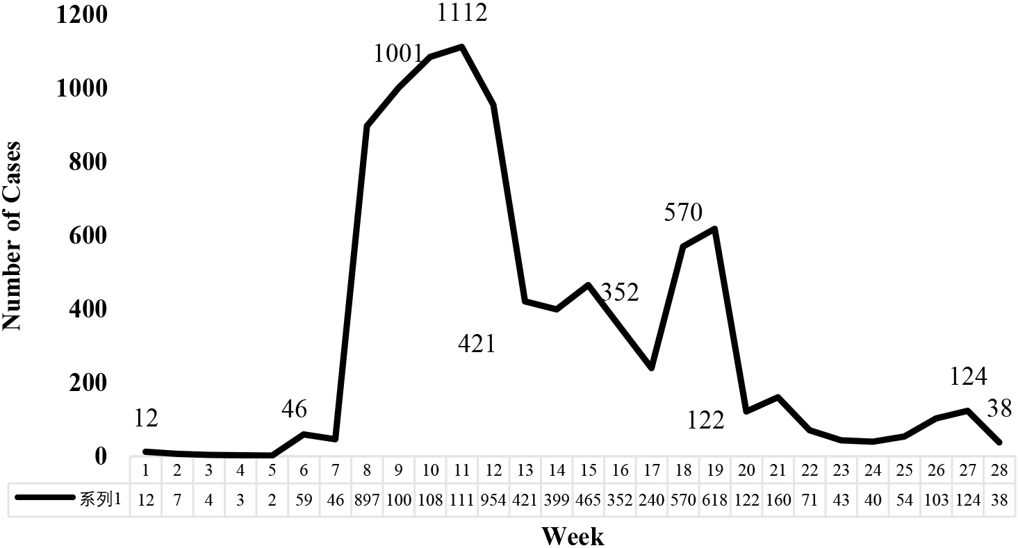
Figure 1.
New COVID-19 infection data in Wave I/II in Malaysia.
This paper attempts to establish a methodological procedure for identifying the best statistical fit for the Malaysian COVID-19 new infection data using the well-known Survival Data Analysis (SDA) procedure. In the current practice the frequency distribution data that provides timely daily COVID-19 counts on new infections, deaths and recovery are still relevant. Complementing the current data practice, the proposed SDA procedure is aimed at reducing the daily frequency counts of COVID-19 new infections data into weekly estimates of shape and scale parameters of the best-fit survival distribution. Upoun establishing the distribution additional analysis like differentiating the experiences of COVID-19 by waves of infections and short-term forecasting on new infections as well as when it is projected to disappear can be carried out. No doubt daily frequency counts on COVID-19 new infections provide timelier estimate, but daily numbers are too many for SDA estimation procedures especially life-table construction which works at best if number of rows are limited to 30 that weekly numbers catered. The fitted distribution, in turn is used to undertake short-term forecasts on new COVID-19 infections using the survival function of the best fit statistical model. The modelling exercise is also used to project the time duration that will take in containing the virality completely under the prevailing conditions. However, the nature of COVID-19 global pandemic is as such subject to changing conditions due to either new variants or mutations that are more aggressive and posing greater life-threatening menace to mankind especially when the borders are open allowing free flow of people and goods. In such circumstances the short-term projections on new COVID infection numbers and when completely it will get mitigated warrants a review of the estimation procedure.
The Malaysian COVID-19 pandemic experiences of Wave I, Wave II and Wave III are used for illustrating the proposed SDA methodological procedure. At this stage Malaysia have been experiencing third wave of COVID-19 pandemic [1]. Despite various shades of cordon sanitaire mitigatory strategies similar to that of Wave I/II that government has put in place beginning 18
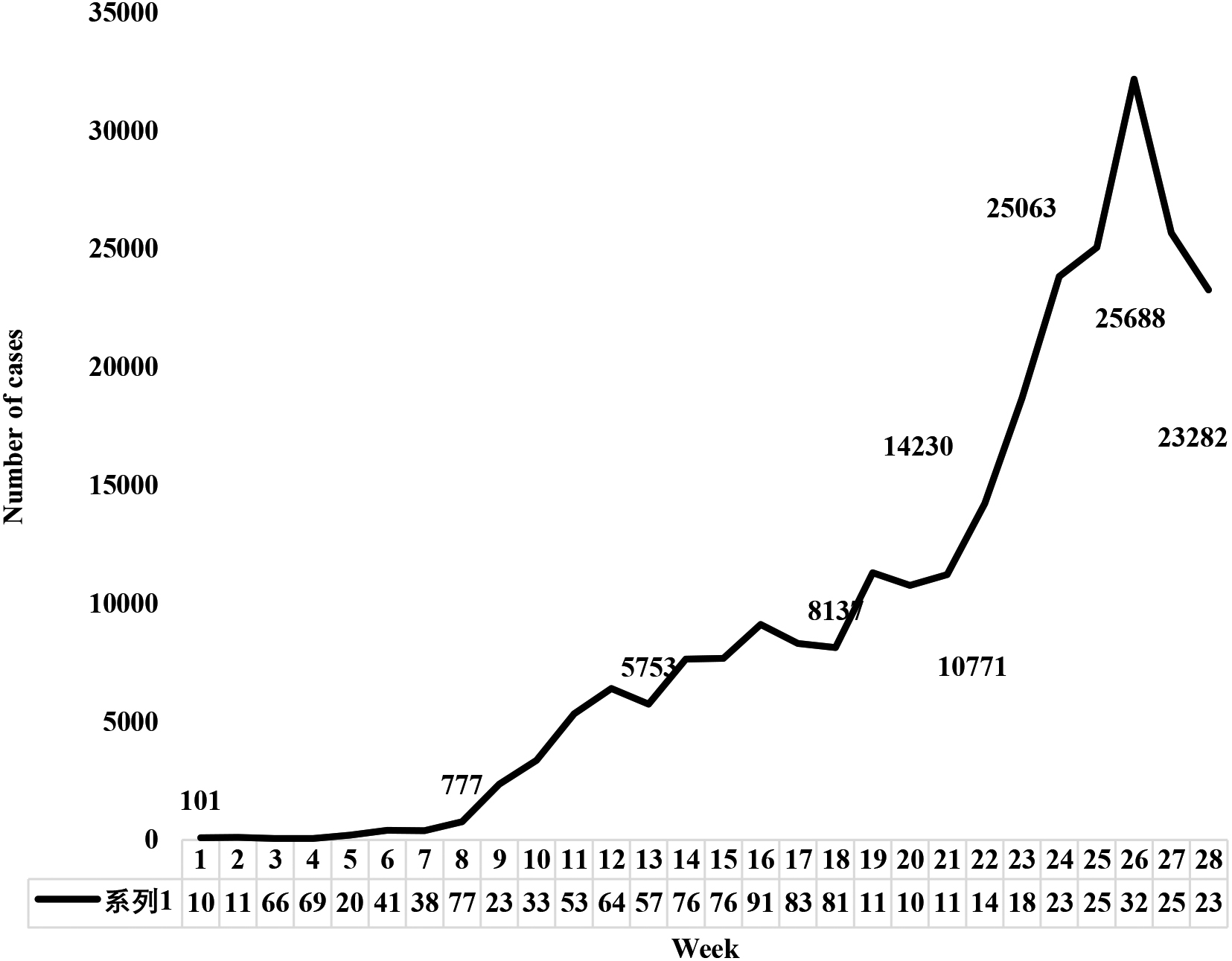
Figure 2.
New COVID-19 infection data in Wave III in Malaysia (on-going).
Currently, the public policy makers, development practitioners, media and academia as well as international organizations are using frequency counts in their policy formulation, planning and advocacy activities. As widely known from past experiences that epidemic or pandemic data are subjected to high fluctuations, skew and kurtosis. Malaysian COVID-19 virus experiences regarding new infections or deaths or recovery after medical treatment are not exception to such erratic phenomena. Compiling data in frequency format and producing summary statistics pertaining to measures of location and dispersion are notably the first statistical activity being undertaken in any data analysis and more so, easier to compile and understand [2, 3] especially the public, media, public policy makers and politicians. Nonetheless, the data presented in frequency counts may exhibit inherent great variations that may not provide meaningful comparisons especially between pandemic waves or geographies or over time [3, 4]. Thus, towards complementing the usage of frequency distribution, this paper explores SDA methodology of converting the COVID-19 new infections frequency counts into scale and shape parameters of best fit survival model distribution. The scale and shape parameters of a statistical distribution are free from unit of measurement and magnitude. The scale measure depicts the extent of virality over time along the horizontal axis and shape parameter determines the rate at which the hazard is increasing and such pure numbers even people with less akin to statistical subject matters able to comprehend the status of virality over time. Indeed, the fitted distribution can be used in producing weekly estimates that become additional information for gauging and monitoring as well as undertake short-term forecasts regarding the virus spirality that will be of interest to mainstream users such as public policy makers, medical professionals and planners, development practitioners in the health sectors, academia and media.
The Figs 1 and 2 shows the number of COVID-19 new infection cases during Wave I/II and Wave III in Malaysia. The analytical investigation is apportioned into two waves of epidemic because the prevailing conditions for the COVID-19 virality and cordon sanitaire measures imposed by the government for containing the virality as well as attitude and behavioural aspect of the population differed greatly between the Wave I/II and Wave III. Pertinently, the total number of new COVID-19 infections over the span of 28 weeks differed greatly, that is 9002 in Wave I/II and 262,596 in Wave III at end of 28th week. Besides that during the Wave I/II period the number of countries affected by COVID-19 virus globally was much lesser than during Wave III which partly experienced increase in the number of cases due to importation of virus from neighbouring countries and by returning Malaysians from overseas [5]. In the same vein, the Movement Control Order (MCO) or cordon sanitaire that were imposed during the Wave I/II period registered with stricter enforcement by the Government authorities in comparison to Wave III, which registered a much more relaxed conditions allowed for economy recovery. The relaxed rules and regulations registered increase in the movement of people for work, free flow of goods, services and workers between localities near and far and resumption of functioning of educational institutions and religious gatherings as well as various shades of social mobility. Indeed, the relaxed conditions paved the way for prolific increase in the virality numbers in Wave III. Reckoning the vast differences in the two waves of epidemic, the analysis prompted to gauge the level of COVID-19 new infections by waves.
2.Working definition of Wave I/II and Wave III
For the Wave I, the WHO for the first time recorded the Malaysian COVID-19 experiences on 25
3.Literature review on Survival Data Analytics (SDA) modelling approach
The study has explored a modelling approach in developing a weekly monitoring system on monitoring the COVID-19 pandemic trend in Malaysia that can be used for analysing and differentiating the new infection experiences and undertake short term forecasts on new infections and when the COVID-19 poised to subside. For studying epidemiological data three types of models namely mathematical, statistical or survival data analysis are usually considered. Each model approach has its own distinct features and characteristics as well as merits and demerits. Among these model approaches, survival data analysis deemed to provide added merits and advantages over the other two. For instance, for analysing small pox disease, [7] Bernouli proposed for the first time a mathematical model using deterministic approach and usage of differential equations [8, 9]. But mathematical modelling demands a sound understanding, appropriate representation and interpretation of mathematical based results of the physical problem [9]. But the weakness in this mathematical approach was the application of the differential equation procedure does not take account of physical units of measurements and random variations associated with unknown factors [9]. Towards overcoming these challenges the cellular automata (CA) mathematical modelling procedure came into practice as it can transform time and space discretely and model the evolution of complex physical systems by incorporating characteristics of the medical conditions, covariates or spatial variables and lags in a lattice structure that the model entails [10]. Nonetheless, sound interpretation of outcomes of mathematical modelling approach still remains much of a challenge for its applicability to COVID-19 type of data, which by and large lack of covariate types of data other than confining to new infections, deaths and recovery numbers [8, 11].
Subsequently, the typical statistical modelling, spatial modelling, space-time approaches and survival modelling that can handle random variations gained stronger footage in modelling exercises. For instance, in Autoregressive Modelling Average (ARMA) framework time lag is estimated using autoregressive process (AR) that treats the observations as a weighted sum of their values at previous time points and the moving average (MA) provides a method that accounts for and corrects for the errors in the previous prediction through a weighted linear sum of previous errors [12]. However, the ARMA models lack statistical efficiency in dealing with issues related to seasonal variations (localized trends), cyclical variations (trends over a longer time period) and irregular fluctuations due to unknown factors and consequently extrapolating future predictions pose modelling difficulties [12, 13]. Similarly, the spatial modelling premises upon homogeneous Poisson process, aims at locating clustering or regularity in recorded events over space and time, estimating and mapping relative risk of the event incidence or identifying clustering around a particular point [14]. Such method is widely applied in spatial epidemiology as the procedures have the ability to model autocorrelation between measurements taken at different spatial lags [15] or applicable to Generalized Linear Model (GLM) framework [16] or dynamic model methodology that models consider non-parametrically non-linear temporal trends [17] in gauging spatial variations. But the spatiotemporal point process statistical modelling tends to average the temporal aspect over time across individuals.
Recognizing the challenges and shortfalls in mathematical and statistical modelling approaches, this paper opted to analyse the COVID-19 new infections data using survival data analysis (SDA). Indeed, the SDA is an aged old procedure that can be traced back to early work on mortality in the seventeenth century when Graunt published the first Weekly Bill of Mortality in London and Healey published the first lifetable [18]. Since then, the lifetable method has been used frequently by actuaries, statisticians, and biomedical researchers in governmental and private agencies in determining life-expectancy at a given age and survival or mortality or relapsed rates in clinical trials and determining insurance premium rates et cetera. In non-medical fields the survival analysis was used in assessing the reliability of military equipment during World War II and subsequently the methodology was used in analysing the reliability of industrial products and devices. In the past four decades, survival analysis has become one of the most frequently used methods for analysing data pertaining to survival times in disciplines ranging from medicine, epidemiology, and environmental health, to criminology, marketing, and astronomy.
In comparison to mathematical and statistical modelling, the survival data analyses offer many distinct merits. First, the purpose of applying SDA procedures to new infections data is to study the time taken for a new infection to happen remising upon probabilistic notion of survival time and hazard functions [19, 50]. Second, the survival time analysis is applicable to situations where the exact survival time may be longer than the duration of the study time (or observation time) [18] because the procedures enable censoring of data either right or left when data are truncated. Applications of survival data analysis in public health or in engineering field or in social science have registered a wide spectrum of usage like estimation of survival distributions, testing hypotheses of equality of two or survival distributions using Gehan’s Generalized Wilcoxon test [20, 21] and the log-rank test [22] and identification of risk or prognostic factors and relating its relationship to the length of disease-free time, survival, or remission [18, 23, 24, 25].
Since the COVID-19 global pandemic came into effect since late 2019, many research endeavours have been undertaken in studying the impact of the COVID-19 virus on human survival using various aspects of survival analysis. To name a few, Salinas et al. [26] and Kyeong [27] investigated impact of COVID-19 on Mexican and South Korean population by expounding Kaplan-Mier curves and Cox proportional model, respectively. Specifically, they examined variables such as age, sex, comorbidities, pregnancy, immune-suppression, smoking, time elapsed between the onset of symptoms and hospitalization, and death, as well as the time elapsed from admission to health care unit to death, development of pneumonia, hospitalization, ICU admissions, intubation, and the type of health service. The case studies concluded that fatality rate was high among males, older age, and those with chronic diseases. Altonen et al. [28] and Eghbal et al. [29] undertook similar studies but focused on USA and Kurdistan population, respectively and concluded that elders with chronic diseases like diabetes need to be under active surveillance and screened frequently.
Atlam et al. [30] deployed machine learning techniques and artificial intelligence for computing infection based on Cox regression modelling aimed at helping hospitals to choose patients who have better chances of survival and predict the most important symptoms (features) affecting survival probability. Interestingly, Yue Zhao and Deepika Dilip [31] used Cox regression procedure on exploring the relationship of the COVID-19 deaths as per Johns Hopkins University publishing and democracy indices as per Economic Intelligence Unit records and concluded that in the public health crisis setting, a democratic government may face more constraints when taking draconian measures against disease control, simply due to its structure and likelihood of opposition. Researchers like Martin Spousta [32] and Bui et al. [33] used parametric models namely linear exponential and Weibull distribution respectively in estimating the incubation period for COVID-19.
Succinctly put, the foregoing literature reviews have indicated that SDA methodology has been registering increasing number of research activities on COVID-19 in many countries using non-parametric or semi-parametric or parametric approaches. In the same vein this exercise scopes its survival analysis to one specific aspect only, that is investigating the time duration incurred in transmission of COVID-19 new infection data from one person to another using either nonparametric or semiparametric or graphical or parametric or combination of approaches. Specifically, attempt is being made in developing a weekly monitoring system on COVID-19 new infections virality by waves by referring to experiences in Malaysia.
4.Merits and demerits of presenting data frequency distribution and basic statistics
Undoubtedly, the compilation of frequency counts depicting COVID-19 pandemic new infections or deaths, or recovery are easily compiled with the support of various reporting sources nationwide in any country including Malaysia. Being a pandemic phenomenon the published daily totals including its cumulative counts are not only concerns of mainstream policy makers, development practitioners and academia but it is also warranted the attention of less statistically orientated ordinary citizens and media in the country. Presenting the data in frequency format obviously become the first option in any statistical activity as it provides a quick glance at the entirety of data conveniently; can spot maximum and minimum values in the data set; and can observe whether they are concentrated in one area or spread out across the entire scale [2, 3, 4, 34]. The industrious users may even monitor the trends whether increasing or decreasing, or remaining at constant level or detect exhibited seasonal and cyclic variations in an attempt to study the emergence of subsequent waves of reappearance of the disease and undertake future projections as well [3, 35]. The advanced users may also convert the numerous frequency counts into single measures of central tendency and dispersion for better understanding of the pandemic phenomena [2, 3, 4, 33].
Data presented in frequency counts are typically constitute numerous observations. However, when presented in time series format the data bound to exhibit high fluctuations in the patterns especially when the series is long. In such data set difficulties may arise in culling out the underlying patterns and trends particularly when the observations are subject to erratic fluctuations that are typically encountered in pandemic kind of data [34, 35]. Besides that, any attempt to compile the data into a grouped frequency format additional concerns arise regarding the number of class intervals, which are fairly arbitrary and determined depending on the size of the timeseries data [2, 3, 4]. If the number of class intervals are too few, it may lead to the loss of much information in the counts and at the same time, if there are too many categories, one may not be able to see the overall picture as one gets bogged down by the excessive details.
Similarly, reducing the numerous COVID-19 daily timeseries observations into representative and dispersion measures like mean or median or mode or standard deviation are likely to encounter several statistical challenges especially whenever spikes or drastic drops in numbers occur regarding the virality of the COVID-19. Moreover, in the presence of extreme values that usually occur in any pandemic data the statistical representation of the data become questionable; skewness may occur in one way or other direction over time due to lack of symmetry; high degree of variation in kurtosis may result due to clustering of cases; mode may become overly sensitive and it can easily be made to “jump around” by varying the limits of the class intervals size and the number [2, 3, 4, 34]. On comparison, in SDA methodology the measures of mean and variance as well as coefficient of variation can be determined for the best fit statistical distribution, besides determining the scale and shape parameters that characterises the nature of the distribution.
Succinctly put, frequency counts with erratic fluctuations may not be statistically efficient for comparing COVID-19 experiences between waves of infection. Such frequency data also may not be suitable for producing meaningful and valid results in undertaking any projections or short-term forecasts. Alternatively, the SDA procedures offer a methodology of reducing the numerous time series-based frequency data into scale and shape parameters of a best-fit survival distribution. The scale and shape parameters are purely numeric numbers and more so, free from order of magnitude and unit of measurements [36] and more aptly, suitable for comparing COVID-19 experiences between waves of infections, despite they differ one from another in terms of intensity of infections or number of deaths or recoveries or duration of epidemic or covariates and prognostics factors influencing the pandemic. But the SDA methodology also offers a statistical procedure for gauging, monitoring, assessing and producing short-term forecasts on COVID-19 new infections by using survival and hazard functions. Historically, the SDA methodology saw its introduction in clinical environment [37, 38, 39, 40] and subsequently used in reliability life testing experiments in engineering and manufacturing plants [37, 41] and as mentioned earlier, today its application is seen in many areas including studying COVID-19 phenomena. As such, in this exercise attempt is being made to measure the virality of new infections of COVID-19 phenomena by waves of new infections experienced in Malaysia in the context of public policy and advocacy activity relevance who are concerned about the trends, patterns, features and characteristics of new virus infections as well as future projections
5.Research objectives
The main objective of this paper is to establish a methodological procedure of gauging, monitoring assessing and evaluating the COVID-19 new infections virality experiences in Malaysia using SDA procedures. Specifically, the SDA methodology is applied in producing and monitoring the weekly estimates of shape and scale parameters for the best fit statistical distribution for the new COVID-19 infections. The weekly results are produced by waves of new infections and assessed in differentiating the trends, features and characteristics inherent to the waves. Having established the weekly estimates the methodology also enables determining short-term forecasts regarding either proliferation or mitigation in new infections and also determining the duration when the COVID-19 viral chain expected to disappear completely.
Currently, frequency-based daily records are used in monitoring and evaluating the COVID-19 phenomena by time or by geography or by waves of infections. As highlighted in the literature review that frequency counts that are highly subjected to presence of extreme values lack inherent statistical inefficiencies for making meaningful evaluations or benchmarking or projections. The SDA procedures that have innate capability of reducing voluminous data that are of diverse characteristics into scale and shape parameters of best fit statistical distribution offer better validity options for evaluation or benchmarking or projections.
This research focuses on Wave I, wave II and Wave II that Malaysia have undergone since the beginning of COVID-19 as a global pandemic. Each wave seemingly has their own distinct features and characteristics in terms of intensity of infections or cordon sanitaire strategies and attitude, behaviour and adherence of people to rules and regulations imposed by authorities. As highlighted earlier the intensity of new infections in Wave III (that is, 262,596 cases) was 25 times more than the combined numbers recorded in Wave I/II (that is, 9002 cases). The rate at which the numbers proliferated between the waves is indeed startling, and warranting a differentiation study pertaining to trends, features and characteristics as well as impact of COVID-19 by Wave I/II and Wave III as highlighted earlier. Reiterating again the trend analysis enable short-term projections on new COVID-19 infections and also predicting when the virality will cease if the current conditions persist. The methodology is dynamic and flexible in the sense projections are subject to review from time to time if there are drastic changes in the virality conditions. Indeed, not only the current data but also a more precise projections on the virality will be of great interest to the mainstream policy makers, medical and public health planners and development practitioners as well as media and academy for their policy, planning, advocacy and communication routines.
Towards this aim the methodological objectives considered the four well-known survival distribution models namely Exponential, Linear Exponential, Weibull and Gompertz distributions [37, 38, 39, 40]. Being a new global phenomenon, the nature of virality of COVID-19 is not known precisely yet. As mentioned earlier, researchers like Martin Spousta [32] and Bui [33] made prior assumptions pertaining to Exponential and Weibull distribution on analysing COVID-19 incubation period, respectively. But, in this exercise attempt is being made to explore combination of graphical, non-parametric lifetable technique, Gehan-Siddiqui semi-parametric procedures and parametric Maximum Likelihood Estimation (MLE) procedure in order to arrive at the more appropriate distribution that describes COVID-19 new infection phenomena in Malaysia.
Specifically, the non-parametric life table technique was used to compute the hazard, cumulative hazard and survival function values pertaining to COVID-19 new infections data that have survival time characteristics that SDA procedures are premise upon. The hazard, cumulative hazard and survival functions of lifetable are in turn used to establish the best fit survival distribution by considering both graphical and regression estimation procedures. Specifically, the hazard and cumulative hazard plots of Exponential, Linear Exponential, Weibull and Gompertz distributions are considered in the graphical procedure and hazard function values are used in the regression estimation procedure. The graphical or semi-parametric procedures deemed to provide only a preliminary indication on estimated values of scale and shape parameters. Refined measures of scale and shape parameters are determined using parametric MLE procedure, which usually statistically considered providing more consistent, efficient and predictable than semi-parametric estimation procedures [42].
The foregoing study objectives depict statistical objectives of determining best fit survival model and its shape and scale parameters. Statistically speaking, the study objective is also include elucidating the meaning of the parameters, that is, scale parameters relate the extent of virality in terms of age or duration, and shape parameters determine rate of hazard of virality growth characterizing the COVID-19 new infections. Interpretatively, these parameters provide surrogate measures for gauging the efficacy of various shades of cordon sanitaire measures that government has put in place. Pertinently, when the rate of hazard is high the incidence of infections is high and vice versa. Thus, effective implementation on the part of authorities and committed and responsible behaviour of people on the other hand are crucial in determining the success rate in containing the COVID-19 chain especially new infections which ultimately can reduce the number of COVID-19 deaths. Unfortunately, the success rate of mitigating the virality of new infections in Wave III was not satisfactory in comparison to Wave I/II.
6.Data source, scope and coverage
For the construction of life-table the study requires data pertaining to number of new COVID-19 infections and deaths by date of reporting. As mentioned, earlier the requisite data are sourced from WHO website and confirmed with Ministry of Health (MoH) records in Malaysia, which is being official statistics. The quality of data is considered valid and reliable as Malaysia has long established public health surveillance system nationwide and more so, the COVID-19 dedicated hospitals are supported with contemporary information communication technology [43].
During the Wave I, Wave II and Wave III a number of zero cases were intermittently reported, meaning no hazard (
7.Methodology
Towards obtaining the best-fit survival distribution and estimation of refined values of scale (
7.1Non-parametric estimation procedure of life-table technique
7.1.1Survivorship function
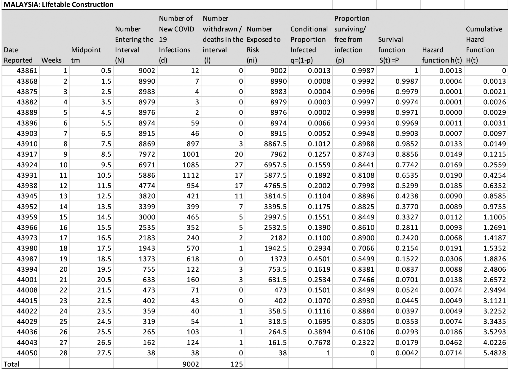
For life-table construction, essentially the SDA methodology premises upon the definition of survival time, denoted as
where
Computationally, for non-censored observations
Where
7.1.2Hazard and cumulative hazard function
The other important function that is typically derived from lifetable is the hazard function
Typically the failure rate refers to death rate in mortality table or end of life span in reliability experiment. Analogously, in this research exercise it refers to “rate of COVID new infection”.
For computation purposes as per actuarial practices, the estimated hazard function
Where,
For computational purposes the cumulative hazard function is derived from the following relationship [37, 38, 39, 40];
Thus, at
Using the large sample approximations, variances of the estimated hazard function
Accordingly, for illustration purposes lifetable for Wave I/II is shown in Appendix I. For the Wave I/II the radix number (
Table 1
Hazard and cumulative hazard and survivorship functions framework
| Survival distribution | Linear relationship of | Scale parameter ( | Shape parameter ( | Survivorship function |
|---|---|---|---|---|
| Exponential distribution | Horizontal line with slope |
| ||
| Linear exponential |
|
| ||
| distribution | ||||
| Weibull distribution |
|
|
|
|
| Weibull distribution |
|
|
| |
| Gompertz distribution |
|
|
|
|
7.2Theoretical framework of Survival Data Analysis (SDA)
The graphical procedure, semi-parametric estimation procedure of regression technique and parametric estimation procedure of using Maximum Likelihood Estimation are based on the parametric assumptions of hazard and cumulative hazard functions of the four well-known survival distributions namely exponential, linear exponential, Weibull and Gompertz [37, 38, 39, 40] and the underpinning formulae of SDA characteristic functions are as per Table 1.
Among the models considered in the framework hazard function of exponential or linear exponential distribution characterises either a constant hazard (
The other popular competing hazard models include log normal distribution, logistics distribution and Gamma distribution but these standard distributions have limitations in fitting some of the real data accurately. For instance, the log normal distribution is characteristically quite similar to Weibull distribution, but it is more applicable to skewed distributions having lower mean values and large variance, in comparison Weibull is more flexible [47]. Similarly, the logistics distribution resembles with normal distribution in shape with mean, median and mode having the same value but with heavier tails or kurtosis than exponential type distribution [48]. Both Gamma and Weibull distributions are generalization of the exponential distribution family which characterises the waiting time as a Poisson process or the time wait until an event occurs. But the hazard or instantaneous failure rate in Gamma distribution is an increasing function of time (
7.3Graphical procedure
As outlined in Table 1, the graphical plotting [38, 39, 40] and are based on values of
7.4Semi-parametric Gehan-Siddiqui regression technique
In undertaking the regression procedure, Gehan and Siddiqui considered linearity relationships of hazard functions as outlined in Table 1 and three types of weights as per below [38, 40]. W
i. W
ii. W
Accordingly, the weighted least square estimates for
Where the weighted least squares estimate for
For identifying the best befitting regression models among the four competing survival models, computation of log-likelihood values based on survival function estimates considered as provided in the columns of the life-table [35, 36, 37], computed as per the formulae below
Thus, the logarithm of the likelihood is:
The model that gives the largest log-likelihood value could be chosen as the best-fit specific model. The best modelfitted will be duly considered for parametric estimation procedure of Maximum Likelihood Estimation procedure in the next step.
7.5Maximum Likelihood Estimation (MLE) procedure
The Weibull Distribution has the density function.
where
Ref. [49] transformed the above equation as follows:
As for such distribution, the MLE of
8.Study findings
The study findings can be summarised as follows:
i) Graphical analysis: The graphical investigation revealed that none of the hazard or cumulative hazard plots provided a perfect or almost near perfect linear fit. Nonetheless a best fit linear trend (
ii) Regression analysis: The regression procedure also indicated that none of the data conformed to Gompertz distribution as per negative values of scale parameter (
iii) Maximum Likelihood Estimation: The Table 2 provides the weekly estimates of scale and shape parameters for gauging, assessing, monitoring, and evaluating Wave I/II and wave III of new COVID-19 experiences in Malaysia, respectively.
Table 2
MLE weekly estimates – Wave I/II and Wave III of Malaysia
Week (t) Wave I and II Wave III Maximum Likelihood Estimation (MLE) Maximum Likelihood Estimation (MLE) Number of cases (f) Shape Scale Number of cases (f) Shape Scale 1 12 0.10816 4.79275E+13 101 0.014084875 1.1132E+103 2 7 0.29468 8563.00000 116 4.2376 1.46030 3 4 0.31689 871.40000 66 2.05070 1.73128 4 3 0.31796 261.90000 69 2.81723 0.81059 5 2 0.46028 18.90000 205 3.09021 0.55475 6 59 1.70089 0.74163 410 3.21747 0.42284 7 46 1.86436 0.52990 389 3.19565 0.34654 8 897 2.76354 0.31852 777 3.19328 0.29069 9 1001 2.94951 0.26062 2369 3.31818 0.24363 10 1085 3.01334 0.22356 3376 3.40629 0.20949 11 1112 3.02715 0.19639 5345 3.47571 0.18335 12 954 3.01171 0.17532 6415 3.51047 0.16314 13 421 2.97754 0.15841 5753 3.51004 0.14718 14 399 2.93737 0.14433 7657 3.50288 0.13390 15 465 2.89202 0.13244 7680 3.48777 0.12273 16 352 2.84965 0.12214 9117 3.47000 0.11315 17 240 2.81137 0.11313 8322 3.44877 0.10486 18 570 2.75577 0.10547 8137 3.42470 0.09763 19 618 2.70652 0.09860 11312 3.40000 0.09125 20 122 2.68137 0.09220 10771 3.37737 0.08556 21 160 2.65329 0.08651 11226 3.35514 0.08047 22 71 2.63074 0.08136 14230 3.33367 0.07589 23 43 2.61037 0.07669 18688 3.31554 0.07173 24 40 2.59027 0.07245 23838 3.30281 0.06793 25 54 2.56833 0.06862 25063 3.29373 0.06446 26 103 2.53957 0.06516 32194 3.28100 0.06452 27 124 2.50821 0.06199 25688 3.26874 0.06458 28 38 2.48956 0.05901 23282 3.25693 0.06463 Table 3
Short term forecasts on COVID-19 new infections in Wave III
Week Scale ( Shape ( Actual count % change between actual and forecast 24 23,838 – 25 0.065156 3.0729 15.3 0.0113565 0.9886435 23,567 25,065 26 0.062336 3.0545 16.0 0.0126461 0.9873539 23,269 32,194 27 0.059738 3.0361 16.7 0.014000 0.986000 22,943 25,688 28 0.057337 3.0147 17.4 0.0154172 0.9845828 22,590 23,282 Average deviation from 25th week to 28th week 29 0.055112 2.9993 18.1 0.0168940 0.9831060 22,889 19,742 16% 30 0.053044 2.9809 18.9 0.0184316 0.9815684 22,469 18,825 19% 31 0.051118 2.9625 19.6 0.0200248 0.97997522 22,017 – – Average deviation from 25th week to 30th week Figure 3.
Weekly shape parameter values by Wave I/II and Wave III in Malaysia.
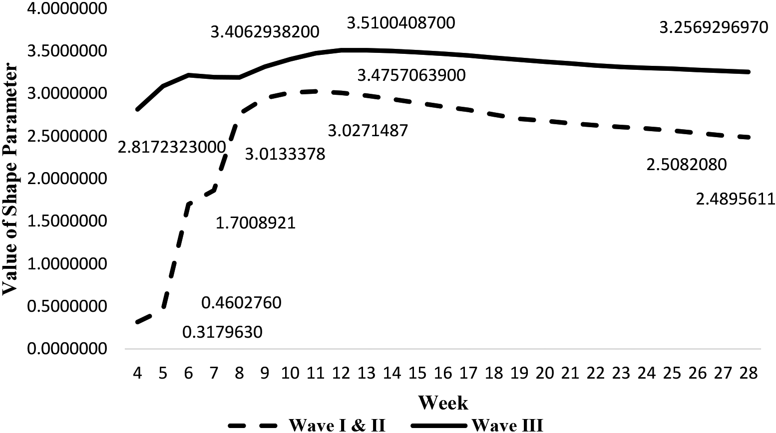
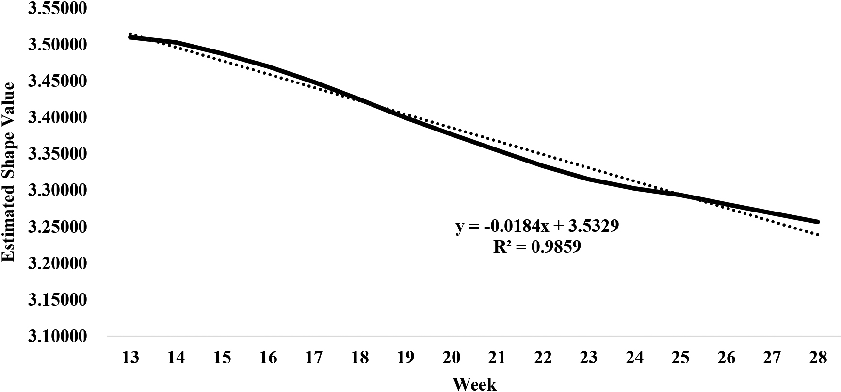
Figure 4.
Downward trend of shape value of COVID-19 in Wave III in Malaysia.
iv) Application of Estimated Shape Parameters for Short Term Forecasts on New Cases of COVID-19 Infections
The weekly trend of shape parameters of fitted Weibull distribution for Wave I/II and Wave III is shown in Fig. 1. The trend is indicating changing direction of the Weibull shape parameter over time. In Weibull distribution the shape parameter depicts the hazard rate behavior or probabilistic chance of a person getting infected by COVID-19 virus at a given time, provided that person is infection free prior to that point. Interpretively, if shape value is less than 1, then the hazard rate decreases with time; if its value is greater than 1, then the failure rate increases with time. When the value of shape parameter is equal to 1, the hazard rate is constant, depicting exponential distribution. Thus, it can be seen in Table 3 as well as in Fig. 1 that the shape value for Wave I/II from week 1 to week 5 was less than 1, indicating the rate of hazard force is lesser in comparison to week 6 onwards where the shape value is greater than one. Similarly, close scrutiny of shape values for Wave III revealed that the rate of hazard value was greater than 1 from week 2 onwards, indicating that the force of aggression for infection was much higher in Wave III from onset than in Wave I/II.
The other pertinent noteworthy feature in Table 3 and Fig. 1 is that the trend or movement of changes in the values of shape parameters. Specifically, it can be observed that the trend of hazard force was increasing until week 11 before it begun to comedown thereafter in the case of Wave I/II; that is increased from 0.10816 in first week to 3.02715 in 11th week as depicted in Table 3 and as well shown graphically in Fig. 3. Similarly, in Wave III the trend of hazard force was on the rise until 12th week before it begun to register a downward trend, that is the shape value increased from 2.050 in third week to 3.51047 in twelfth week (see Table 3). It is also duly acknowledged in the analysis that Wave I/II COVID-19 new infections phenomena were over, thus no further analysis explored. In the case of Wave III, which has been on-going at the point of analysis the trend showed that it has been gradually declining from 13th week onwards. Thus, for short-term forecasting purposes the trend fitting was done for the downward trend from Week 13 onwards as reflected in Fig. 4. It can be seen that linear trend provided the best fit of
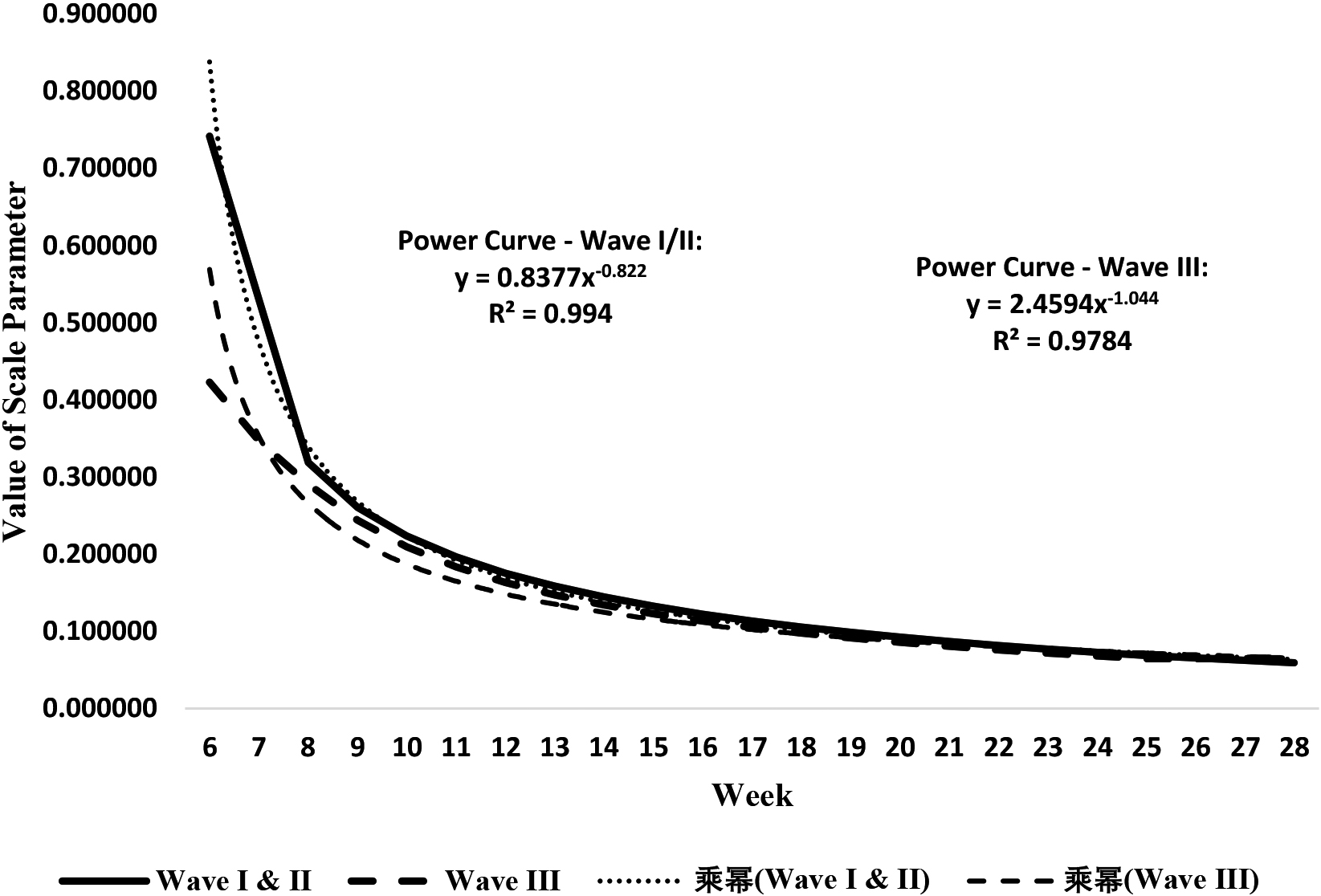
Figure 5.
Visualization of trend for scale parameter values by week: Wave I/II and Wave III Malaysia.
Based on the assumption of survival function
where
The forecasts exercise was undertaken at week 28. In order to validate the accuracy of the results the exercise also estimated values of scale and shape as well as the survivorship function values for three prior weeks, that is week 25, 26 and 27 and accordingly the forecast numbers on new infections were determined. These numbers in turn were compared against the actual counts of new infection and accordingly the percentage of over or under estimation were determined as shown in Table 3; the deviation ranged from underestimation of 3.0% for 28th week to 27.7% for 26th week when there was a sudden surge in the number of new infections occurred. The average of percentage of under estimation deviation over the preceding four consecutive weeks was 11.8%; excluding week 26 the average was only 6.5%, which is generally an acceptable range in projection exercise.
Based on the current prevailing conditions, the forecast results on new COVID-19 infections for the next two weeks are also shown in Table 3. As it can be seen in the Table 3 that the number of new infections for the week 29 was 22,889 cases, which compared against actual count of 19,742 cases, which is considered over estimation by 16%. Similarly, for the week 30 the estimated number of cases was 22,469 and actual was 18,825 cases, giving rise to 19% in over estimation. The implicit challenge in this methodology is that the forecast estimation is sensitive to drastic changes in prevailing conditions of virality like being seen in week 26, 29 and 30. For example, the actual counts on week 27 reported as 25,668 which dropped to 23,282 cases in week 28, that is a drop of 9.4% and comparing against week 29 that registered 19,742 cases resulted further drop by 15%. Acknowledging the sensitivity of the methodology, in practice the short-term forecasts warrant review from time to time especially when significant changes are observed in the number of new infections cases.
v) Application of Estimated Scale Parameters for Short Term Projections on COVID-19 Reduction in New Infections
As acknowledged earlier that the Wave I/II COVID-19 infection were over for Malaysia. Nonetheless, the visual trend for scale parameter values for Wave I/II and Wave III is shown in Fig. 5. Further examination separately for each wave, as depicted in Fig. 5 the analyses revealed that the power curve function (
As it can be seen in Fig. 5 that the estimated value of scale gradually decreased with progression of time, indicating prolongation in the disappearance of the virality of the COVID-19 new infections. It can be seen in Table 3 that the scale values for Wave I/II were very high for the first five weeks and only from week 6 onwards the scale value that recorded 0.7413 thereafter declined incrementally until it reached value of 0.05901 in 28th week. Similarly in Wave III the scale value registered a stable measure of 0.81059 at the 4th week and thereafter slowly declined until it reached 0.06463 by 28th week. In both Wave I/II and Wave III the initial scale values were high probably due to small number of cases of new infections as the scale measure is inversely proportional to number of cases as per MLE formula. At the early stages of COVID-19 pandemic understandably the government of Malaysia was attempting to implement various shades of cordon measures in containing the virality spread and with concerted support of masses the number of infections in Wave I/II begun to come down continuously after reaching its maximum of 1112 cases at 12th week. Whereas the scenario in Wave III is different and the cases of new infection have been continually on the rise and as such the number reached 23,282 by the 28th week. The key difference is that Wave I/II saw stricter implementation of cordon sanitaire measures and in Wave III the rules and regulations of cordon sanitaire measures have been much relaxed in lieu of reviving the ailing economy growth despite health menace to the population.
In Wave I/II only essential services of economy especially public utility services, working from home and online education were allowed to function. While in Wave III, some of the relaxed conditions include opening up of all economic sectors, schools and religious institutions, worship centres, social gatherings and greater social mobility et cetera, but with stricter standard operating procedures (SOP) regarding maintaining social distancing, wearing face mask, frequent sanitization of hands, gauging body temperature and recording Q-R code for technology tracing. Indeed, the Government has been facing challenging times in balancing the economy growth and maintaining the health of the population in such a global pandemic scenario.
9.Conclusion
Succinctly put, the foregoing survival data analysis procedures regarding the COVID-19 new infections data have realized a number of statistical benefits. First, the research exercise has established a methodology of analysing the COVID-19 new infection using SDA procedures that are founded upon the probabilistic notion of survival time and hazard function. Second, the SDA procedure deployed non-parametric, semi-parametric and parametric as well as graphical procedures in determining the appropriate statistical distribution that deemed to provide best fit, instead of pre-empting its assumptions. Accordingly, the analysis showed the Weibull distribution provided the best fit among the well-known distributions considered in epidemiological kind of studies. Third, the methodology reduced the voluminous time series daily frequency counts of COVID-19 new infections data into weekly class intervals data not exceeding 30 rows that deemed appropriate for efficient application of life-table technique. Fourth, the life-table in turn enabled the estimation of hazard and survival function values for the new infections data, which through the semi-parametric regression and MLE procedures enabled the estimation of scale and shape parameters for the fitted Weibull distribution for both Wave I/II and Wave III in the case of Malaysian experience. Fifth, being free from unit of measurement and order of magnitude [36], the scale and shape parameters of Weibull distribution provided meaningful comparisons of COVID-19 new infection experiences between Wave I/II and Wave III. Specifically, the scale and shape parameters for Wave I/II was 0.05901 and 2.48956 and for Wave III was 0.06463 and 2.5693, respectively. Much higher hazard force as reflected in larger shape values in Wave III is due to weaker control in the implementation of cordon sanitaire measures imposed by Government in containing the virality, in comparison to Wave I/II. Sixth, by fitting appropriate trends for the estimated weekly results of scale and shape parameters the survival function of Weibull distribution enabled the short-term forecasts on new infections, which showed decline in the trend incrementally from 23,282 cases in 28th week to 22,017 cases in 31st week and poised to decline further under the current prevailing conditions unless abrupt changes occur in the trend Seventh, the cumulative hazard function of Weibull distribution provided a basis for estimating the duration when the virality of new COVID infections is likely to disappear completely and the results showed that it may stretch over another 19.6 weeks as per estimation at 28th week Lastly, the foregoing SDA methodology provides a complementary measure in addition to frequency counts distribution and more so, the methodology can be an exemplary model for other countries to emulate.
References
[1] | WHO (2020). Coronavirus disease (COVID-19) Weekly Epidemiological Update and WHO (January 2021). Coronavirus disease (COVID-19) advice for the public. https://www.who.int/emergencies/diseases/novel-coronavirus-2019/advice-for-public. This content is last updated on 6 January 2021. |
[2] | Manikandan S. Frequency distribution. Journal of Pharmacology and Pharmacotherapeutics. (2011) ; 2: (1): 54. doi: 10.4103/0976-500x.77120. |
[3] | Owen F, Jones R. Statistics (2nd ed.). Longman London and New York. |
[4] | Kapur JN, Saxena HC. Mathematical Statistics. Fourth Edition. S. Chand and Company Limited. (1999) . |
[5] | Abdullah JM, Wan Ismail WFN, Mohamad I, Ab Razak A, Harun A, Musa KI, Lee YY. A critical appraisal of COVID-19 in Malaysia and beyond. Malaysian Journal of Medical Sciences. 27: (2): 1-9. doi: 10.21315/mjms2020.27.2.1. |
[6] | Wagner AL. What Makes a “Wave” of Disease? An Epidemiologist Explains. The Conversation. Chicago. (2002) . |
[7] | Bernoulli, Daniel. Reflexions sur les avantages de l’inoculation. Mercure de France, June issue, 173-190. Gani J. (1978). Some problems of epidemic theory (with discussion). Journal of the Royal Statistical Society Series A. 1760; 141: 323-347. |
[8] | Bailey NTJ. The mathematical theory of infectious diseases and its application. London: Griffin: Thom, R. 1975: Structural stability and morphogenesis. Reading, Massachusetts: Benjamin. Progress in Human Geography. (1983) ; 7: (3): 442-444. doi: 10.1177/030913258300700313. 1975. |
[9] | Thomas RM. Blending Qualitative and Quantitative Research Methods in Theses and Dissertations. Thousand Oaks, CA: Corwin Press. Journal of Mixed Methods Research. (2007) ; 1: (3): 295-297. doi: 10.1177/1558689806294476. 2003. |
[10] | Fuentes M, Kuperman M. Cellular automata and epidemiological models with spatial dependence. A Statistical and Theoretical Physics. (1999) ; 267: : 471-486. doi: 10.1016/S0378-4371(99)00027-8. |
[11] | Sirakoulis G, Karafyllidis I, Thanailakis A. A cellular automaton model for the effects of population movement and vaccination on epidemic propagation. Ecological Modelling. (2000) ; 133: : 209-223. doi: 10.1016/S0304-3800(00)002945. |
[12] | Box G, Jenkins G. Time Series Analysis: Forecasting and Control. San Francisco. Holden-Day. (1970) . |
[13] | Chatfield C. The Analysis of Time Series: An Introduction. Chapman and Hall. CRC Press, Boca Raton. (2004) . |
[14] | Lawson AB, et al. Spatial mixture relative risk models applied to disease mapping. Statistics in Medicine. (2002) . |
[15] | Bailey TC, Gatrell AC. Interactive spatial data analysis in medical geography. Social Science & Medicine. (1996) ; 42: (Issue 6): 843-855. |
[16] | Bernardinelli L, Clayton D, Pascutto C, Montomoli C, Ghislandi M, Songini M. Bayesian analysis of space – time variation in disease risk. Statistics in Medicine. (1995) ; 14: (Issue 21-22). |
[17] | KnorrHeld L, Besag. Modelling risk from a disease in time and space. Statistics in Medicine. (1998) ; 17: : 2045-2046. |
[18] | Elisa TL, Oscar TG. Survival analysis in public health research. Annual Review of Public Health. (1997) 18; 1: : 105-134. |
[19] | Cox DR, Oakes D. Analysis of Survival Data. Chapman and Hall. London. (1984) . |
[20] | Gehan EA. A generalized two-sample Wilcoxon test for doubly-censored data. Biometrika. (1965) ; 52: : 650-53. |
[21] | Gehan EA. A generalized Wilcoxon test for comparing arbitrarily singly-censored samples. Biometrika. (1965) ; 52: : 203-23. |
[22] | Peto R, Peto J. Asymptotically efficient rank invariant procedures. J. R. Statist. Soc. (1983) ; A135: : 185-207. |
[23] | Fenn P, McGuire A, Phillips V, Backhouse M, Jones D. The analysis of censored-treatment cost data in economic evaluation. Med. Care. (1995) ; 33: : 851-63. |
[24] | Saeki S, Ogata H, Okubo T, Takahashi K, Hoshuyama T. Return to work after stroke: A follow-up study. Stroke. (1995) ; 26: : 399-401. |
[25] | Cox DR. Regression models and life tables. J. R. Statist. Soc. (1972) ; B34: : 187-220. |
[26] | Salinas-Escudero G, Carrillo-Vega MF, Granados-García V, et al. A survival analysis of COVID-19 in the Mexican population. BMC Public Health. (2020) ; 20: : 1616. doi: 10.1186/s12889-020-09721-2. |
[27] | Kyeong Hyang Byeona, Dong Wook Kimb, Jaiyong Kimc, Bo Youl Choia, Boyoung Choid, Kyu Dong Chob. Factors affecting the survival of early COVID-19 patients in South Korea: An observational study based on the Korean National Health Insurance Big Data International. Journal of Infectious Diseases. Elsevier. (2021) . |
[28] | Altonen BL, Arreglado TM, Leroux O, Murray-Ramcharan M, Engdahl R. Characteristics, comorbidities and survival analysis of young adults hospitalized with COVID-19 in New York City. PLoS ONE. (2020) ; 15: (12): e0243343. doi: 10.1371/journ. |
[29] | Eghbal Zandkarimi Ghobad Moradi, Behzad Mohsenpour. The Prognostic Factors Affecting the Survival of Kurdistan Province COVID-19 Patients: A Cross-sectional Study from February to May 2020. International Journal of Health and Policy Management. (2020) . |
[30] | Atlam M, Torkey H, El-Fishawy N, et al. Coronavirus disease 2019 (COVID-19): survival analysis using deep learning and Cox regression model. Pattern Anal Application. (2021) . doi: 10.1007/s10044-021-00958-0. |
[31] | Yue Zhao, Deepika Dilip. Survival Analysis of COVID-19 on Democracy with Cox Proportional Hazards Model. Atlas Statistical Research, King of Prussia, PA, United States. Memorial Sloan Kettering Cancer Center, New York, United States. (2020) . |
[32] | Martin Spousta. Parametric analysis of early data on COVID-19 expansion in selected European countries doi: 10.1101/2020.03.31.20049155. (2020) . |
[33] | Bui LV, Nguyen HT, Levine H, Nguyen HN, Nguyen T-A, Nguyen TP, et al. Estimation of the incubation period of COVID-19 in Vietnam. PLoS ONE. (2020) ; 15: (12): e0243889. doi: 10.1371/journal.pone.0243889. |
[34] | In J, Lee S. Statistical data presentation. Korean Journal of Anesthesiology. 70: (3): 267. doi: 10.4097/kjae.2017.70.3.267 ISSN 0277-9536. |
[35] | Anderson TW. The Statistical Analysis of Time Series (1st ed.). Wiley-Interscience.coronavirus-2019/situation-reports. (1994) . |
[36] | Ramasamy R. Measuring Information and Knowledge Development in the New Millennium [Master’s thesis].– Research thesis submitted for the award of Master of Philosophy by Multimedia University (MMU), Cyberjaya Multimedia University, Malaysia in 2008. |
[37] | Kleinbaum DG, Klein M. Survival Analysis: A Self-Learning Text. (3rd ed.). Springer-Verlag. (2012) . |
[38] | Lee ET. Statistical methods for survival data analysis. Lifetime Learning Publications. (1980) . |
[39] | Lee ET. Statistical Methods for Survival Data Analysis (Wiley Series in Probability and Statistics) (2nd ed.). Wiley-Interscience. (1992) . |
[40] | Lee ET, Wang JW. Statistical Methods for Survival Data Analysis (Wiley Series in Probability and Statistics) (3rd ed.). Wiley-Blackwell. (2003) . |
[41] | Sinha SK. Reliability and Life Testing. Wiley Eastern Limited. Bombay, India. (1986) . |
[42] | Fernández-Sainz, Ana. An Empirical Investigation of Parametric and Semiparametric Estimation Methods in Sample Selection Models. Journal of Quantitative Methods for Economics and Business Administration. (2010) . |
[43] | Shah AUM, Safri SNA, Thevadas R, Noordin NK, Rahman AA, Sekawi Z, Ideris A, Sulta MTH. COVID-19 outbreak in Malaysia: Actions taken by the Malaysian government.International Journal of Infectious Diseases. (2020) ; 97: : 108-116. doi: 10.1016/j.ijid.2020.05.093. |
[44] | Ramasamy R. Survival Data Analysis of the Flow of Vital Event Forms in Peninsular Malaysia. [Paper presentation]. Seminar paper submitted as a part of requirements for Post Graduate Course in Population Studies, International Institute of Population Sciences, Deonar, Bombay. (1990) . |
[45] | Robert E. Ricklefs, Alex Scheuerlein, Biological Implications of the Weibull and Gompertz Models of Aging. The Journals of Gerontology: Series A. 1 February (2002) ; 57: (Issue 2): B69-B76. doi: 10.1093/gerona/57.2.B69. |
[46] | Juckett D, Rosenberg B. Comparison of the Gompertz and Weibull functions as descriptors for human mortality distributions and their intersections. Mechanisms of Ageing and Development. (1993) ; 69: : 1-31. doi: 10.1016/0047-6374(93)90068-3. |
[47] | Kundu D, Manglick A. Discriminating between the Weibull and log-normal distributions. (2004) . doi: 10.1002/nav.20029. |
[48] | Balakrishnan N. Handbook of the Logistic Distribution, Marcel Dekker, New York. (1992) . |
[49] | Gehan EA, Siddiqui MM. Simple Regression Methods for Survival Time. |
[50] | Murray S, Tsiatis AA. Nonparametric survival estimation using prognostic longitudinal covariates. Biometrics. (1996) ; 52: : 137-51. |
Appendices
Appendix 1