
A geographically weighted regression approach to examine the dynamics of fertility differentials across Africa
Abstract
Studies have shown that fertility rate in Africa is still among the highest in the world. However, there are few spatial investigations into the variation of fertility rate and its determinant in Africa. This study aimed to examine the spatial distribution of fertility rate as well as highlight its significant determinants. Ordinary Least Squares (OLS) regression was carried out on dataset for 53 African countries on Total Fertility Rate (TFR) and eleven determinant factors to obtain a best model, which was then used for Geographically Weighted Regression (GWR). The study showed that TFR was significantly influenced by adolescent fertility rates, contraceptive prevalence rates and gross domestic product per capita. GWR model diagnostics of Akaike Information Criterion and adjusted R-squared showed that GWR fitted TFR in Africa better than OLS model. Also, countries around Middle to Western Africa comprising Burundi, Democratic Republic of the Congo, Central African Republic, Chad, Nigeria, Niger, Benin, Burkina Faso and Mali, were regions with high TFRs that impacted Africa’s positive TFR spatial autocorrelation. More intense works could therefore be carried out in these countries to manage the identified significant factors affecting TFR to address the negative consequences of high TFR in Africa.
1.Introduction
There are several studies on fertility rate and its determinants in Africa [1, 3, 2], yet many works are currently being undertaken to understand the population dynamics of the African continent and the various issues associated with its population such as fertility rate. Most of such studies on fertility reported on the factors associated with the perception and behaviour of families in Africa and their desire for particular family size [4]. The focus has also shifted to fertility transition as many nations of Africa with large population growth hitherto are beginning to see a downward movement in fertility rate as was observed in Asia and Latin America [5, 1].
Additionally, fertility transitions in Sub-Saharan Africa have also been studied [3, 5]. Sneeringer [3], studied cohort fertility trends in 30 sub-Saharan African countries in order to discern fertility patterns over past five decades. The study was a construction of a panel using the fertility histories of survey respondents in order to understand how women born at different periods in time may alter their fertility patterns. It concluded that many countries showed increases in fertility rates in the 1960s and 1970s, and then a decline by later cohorts. The overall pattern is that countries that have initiated declines do not later see sustained increases in fertility. While countries vary in fertility levels and trends, 26 of the 30 countries studied showed at least a 10% decline in fertility for at least one age group cohorts. These findings suggest that most countries exhibit sustained or progressively larger fertility declines in age groups between 20 and 34 [3]. Hence, women later in middle reproductive age group (25 years and over) have larger fertility decline than those in younger age groups.
Westoff et al. [4] also studied fertility trends indicators in Sub-Saharan Africa in which the changes in country characteristics and their relationships with changes in fertility indicators were examined. The Change in the Total Fertility Rate (TFR), they noted were affected by changes in age at first marriage of women, desired number of children, and use of contraception, which they also noted were in turn affected by trends in health and socio-economic factors such as infant mortality rate, rural-urban residence, years of schooling, exposure to mass media (television and radio) and economic status [4]. The study concluded that reductions in the desired number of children and increases in the use of modern contraception were the most important, while increase in age at first marriage had a minor role. These determinants were found to be influenced by the increasing access to education, urbanization, and mass media exposure [4].
This study is premised on the availability of geographic and demographic data which gives the opportunity of analyses that combines both types of data. These analyses are referred to as spatial demography. Matthews and Parker [6] have defined this concept of spatial demography as the spatial analysis of demographic processes and outcomes. A comprehensive review of the advanced spatial analytic methods and the insights that can be gained by applying a spatial perspective to demographic processes and outcomes is given [6].
Methodically, the use of linear regression allows the model parameters to be considered identical across various areas or regions under study, but the idea of uniformity across areas or regions is usually unrealistic [7]. If the parameters vary significantly across regions, a global estimator such as the ordinary least square estimator will not show the geographical dimensions of the response variable [8]. In case of demographic data, the linear regression is insufficient in telling the entire story of the variable of interest in terms of its distribution across regions. Local linear regression with the spatial component referred to as Geographically Weighted Regression (GWR) has been obtained for geographic data [7].
This study seeks to apply GWR to fertility dynamics across space in Africa as scarcely any study has looked at fertility dynamics holistically across Africa geographically. The study focuses on TFR as the dependent variable and some of its quantifiable determinants viz-a-viz life expectancy at birth, gross domestic product per capita, infant mortality rate, contraceptive prevalence rate, unmet need for family planning, adolescent fertility rate and female labour participation and how they interact and change across space in Africa. The analysis begins with univariate data description, the bivariate analysis showing relationships between the dependent and independent variables. Linear regression (OLS) model was fitted to the dataset and used to compare the GWR model for the dataset. Lastly, the GWR is used to explain the relative contribution and the statistical significant factors that contribute to TFR examining how spatially consistent relationships between the TFR and each determinant variable are across the Africa.
2.Materials and methods
2.1Data source and limitation
The challenge of data has been a major concern highlighted in almost all studies about Africa due to the cost in time and money to conduct censuses and surveys. Many international donors sponsor censuses and surveys in Africa which are carried out in many countries and done in different time periods in different countries. So it is quite difficult to get dataset for all countries in the same period of time from the same survey (such a survey would be very huge and too expensive). The dataset used in this study on TFR and the other factors such as infant mortality rate (IMR), adolescent fertility rate (AFR), life expectancy at birth, GDP per capita and female labour participation were from the World Bank Open Data [9] for the period of 2017. Data on Contraceptive prevalence rate, demand for family planning and unmet need for family planning were obtained from United Nations, Department of Economic and Social Affairs, Population Division [10].
Disputed territories of Western Sahara and Somaliland are not included in the analysis as data on these places were not available. The observations of each variable reported in the data represent specific geographical locations where the information on each variable had been taken. The dataset does not contain observations for the geographical divisions in each country. These observations are taken to representative the centroids of the countries. In this case, the underlying assumption is that the distribution of the variable within each country is sufficiently homogeneous to approximate it to a single observation.
The several sources of data used, means different samples and experimental conditions as opposed to data set from a single source which would have been collected under the same samples and experimental conditions, may account for some margin of error. Albeit, the situation may be a blessing in disguise, when the assumption of randomization for statistical analyses is considered, the data set are of the same period but different samples and experimental conditions, so it can be said that sampling fluctuation will be reduced.
The metadata for each of the variables are given thus:
• Total fertility rate (TFR): number of births per woman. This represents the number of children that would be born to a woman if she were to live to the end of her childbearing years and bear children in accordance with the prevailing age-specific fertility rates (ASFR) of the specified year.
• Adolescent fertility rate (AFR): number of births per 1000 women aged 15–19 years.
• Infant mortality rate (IMR): the number of infants dying before reaching their firth birthday, per 1,000 live births in a given year.
• Contraceptive prevalence rate (CPR): percentage of women aged 15–49 years currently using a contraceptive per 1000 women in the same age group
• Use of Family planning: percentage of women currently using a modern method of contraception among all women of reproductive age group (15–49 years).
• Unmet need for family planning: percentage of women who affirm that they want to stop or delay childbearing but are not using any method of contraception to prevent pregnancy.
• Life expectancy at birth: the number of years a new born infant would live if the prevailing patterns of mortality at the time of its birth were to stay the same throughout.
• Gross domestic product (GDP) per capita (US$): the sum of gross value added by all resident producers in the economy plus any product taxes and minus any subsidies not included in the value of the product.
• Female labour participation: percentage of female labour force (15–64 years). It defines the extent to which women are active in the labour force.
2.2Spatial autocorrelation
Autocorrelation is the association of a variable with itself when observations on the variables are obtained in different time periods or in space. Spatial autocorrelation has been defined as the positive or negative correlation of a variable with itself due to the spatial location of the observations [11]. Analysis of spatial autocorrelation enables quantified analysis of the spatial structure of the studied variable whose value is related to its other values from neighbouring regions. The presence of spatial autocorrelation either means that similar values of the variables are geographically clustered together or values far away are more similar to values in nearby locations. Spatial autocorrelation indices such as the Moran index and the Geary index make it possible to assess spatial structure of variables.
This study employs the Moran index which takes into account the variances and covariances with the difference between each observation and the average of all observations. In the literature, Moran’s index is often preferred to that of Geary due to greater general stability [11, 12].
Given observations,
(1)
where
Spatial autocorrelation value is obtained using the Moran’s test which tests the null hypothesis of absence of spatial autocorrelation for a variable, in which case the values of the variable are randomly assigned to the spatial units in order to calculate the test statistic. The Moran’s index from the test is a single measure which represents the entire data.
2.3Geographically weighted regression
In order to seek the factors that relate with TFR and examine the spatial consistency in the relationship between the factors and TFR across Africa, GWR is employed on the dataset. GWR is a regression analysis technique that employs the traditional regression framework to geographical data by allowing the estimation of parameters at each location instead of parameters at a single summary for the entire space. In other words, GWR runs a regression for each location, instead of a sole regression for the entire study area.
The coefficients of GWR are not fixed but depend on coordinates of observations, that is, the coefficients of the explanatory parameters form continuous surfaces that are assessed at certain points in space [8]
(2)
where the parameters
In estimating the coefficients, using fixed-coefficient model and including only observations close to point
(3)
at any given point, if weights are given to observations with weighted least squares, then
(4)
and
where
The weight of observations decreases with the distance of the observation to the point
Gaussian Kernel,
where
2.3.1Defining neighbourhoods
The definition of neighbourhood consists in selecting the
The nbdists function of the ‘spgwr’ package in CRAN is used to calculate the vector of distances between neighbours. It makes it possible to determine the maximum distance
Figure 1.
Nearest neighbours spatial relationship of observations of total fertility rate across Africa.
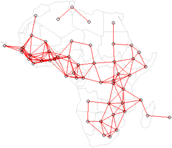
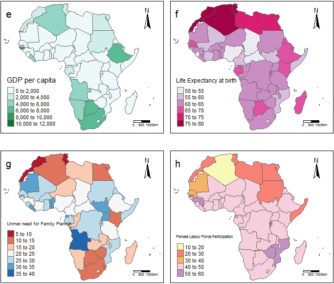
Figure 2.
Spatial distribution of variables across Africa including non-contiguous areas (a) shows the 2017 data on total fertility rate (b) shows the 2017 data on adolescent fertility rate (c) shows the 2017 data on infant mortality rate (d) shows the 2017 data on percentage contraceptive prevalence rate by women of reproductive age.
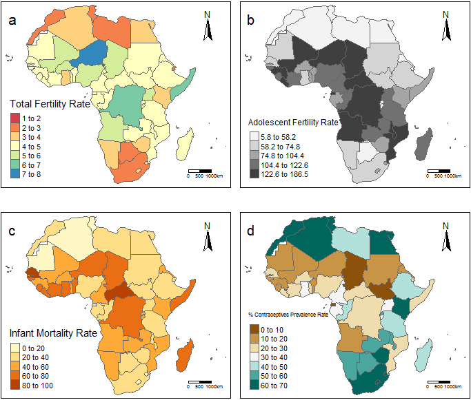
Figure 3.
Spatial distribution of variables across africa including non-contiguous areas (e) shows the 2017 data on gross domestic product per capita (US Dollars) (f) shows the 2017 data on life expectancy in years (g) shows the 2017 data on percentage of women of reproductive age with unmet need for family planning (h) shows the 2017 data on percentage of female labour force participation.
The observations are centroids which are specific locations representative of each country of Africa. In this case, the underlying assumption is that the distribution of the variable within each country is at least homogeneous enough to be estimated by a single observation. Figure 1 shows the neighbourhood distribution across space showing the links of neighbours of the observations taken for Africa as defined by the nearest neighbours distance spatial relationship.
2.4Spatial distribution of variables
Figures 2 and 3 show the spatial distribution of the 2017 observations of the eight variables including TFR across Africa. These observations are a single value for each of the 53 countries for the analysis on the eight different variables, and represent the average values for all the divisions of a country. It can be seen that as at 2017, the West African sub-region had the highest TFR in Africa, with Middle Africa following. Southern and Northern Africa have the lowest fertility rates in the continent. This pattern can also be seen in the distribution of AFR as the highest rates are within Western, Middle and Eastern Africa, while Northern and Southern Africa have the lowest adolescent births.
IMR, CPR, and unmet need for family planning show the same spatial distribution pattern across Africa. Northern and Southern Africa have the lowest infant mortality rates and unmet need for family planning compared to other sub-regions.
The gross domestic product per capita for countries in Western, Middle and Eastern Africa is on the average less than US$2,000, with exception of the Island of Mauritius that recorded over US$10,000 in gross domestic product per capita. Southern and Northern Africa recorded gross domestic product per capita in 2017 between US$4,000 and US$8,000, except for Libya, which has been in unrest and political crises since 2011. Life expectancy at birth is much higher in Northern Africa than other regions, Fig. 2f. Figure 2h shows that the percentage of female labour force participation in 2017 was almost evening out across Western Middle, Eastern and Southern Africa, with exceptions of countries like Guinea, Burundi, Rwanda, Mozambique and Zimbabwe where the percentage of women in labour force is between 50% and 60%.
2.4.1Descriptive statistics of observations on the variables
Table 1 shows the descriptive statistics for the various factors assumed to be associated with TFR. This summary shows average values for each of the variables based on the data obtained during the period 2017 for Africa. From the results, the unweighted average TFR in 2017 was about 4 children per woman, the average life expectancy was 63 years and a median gross domestic product per capita of US$1,232.79. The unweighted average of 49.61% women in Africa were using modern family planning method. CPR stood at 34.9% among women in reproductive years (15–49 years), while unmet need for family planning was at 22.7%.
Table 1
Summary statistics on data
| Variables | Mean | SD | Median | Min | Max | SE |
|---|---|---|---|---|---|---|
| Total fertility rate (TFR) | 4.28 | 1.14 | 4.39 | 1.44 | 7.00 | 0.16 |
| Life expectancy at birth | 63.22 | 5.99 | 63.04 | 52.24 | 76.50 | 0.82 |
| GDP per capita | 2212.92 | 2423.01 | 1312.37 | 228.00 | 10484.91 | 332.83 |
| Infant mortality rate (IMR) | 44.41 | 19.22 | 41.50 | 10.60 | 86.50 | 2.64 |
| % Contraceptive prevalence rate | 35.92 | 19.94 | 30.70 | 6.50 | 67.60 | 2.74 |
| Unmet need for family planning | 22.63 | 7.18 | 23.50 | 9.50 | 36.70 | 0.99 |
| Use of modern family planning | 50.00 | 19.98 | 44.70 | 16.20 | 85.80 | 2.74 |
| Adolescent fertility rate | 89.73 | 42.45 | 89.09 | 5.77 | 186.54 | 5.83 |
| Female labour force participation | 43.07 | 8.88 | 46.54 | 17.88 | 53.21 | 1.22 |
Table 2
Means of various Indicators by sub-region of Africa
| Sub-region of Africa | No of countries | Total fertility rate | Life expectancy | GDP per capita | Infant mortality rate | % Contraceptive prevalence rate | Unmet need for family planning | Modern family planning method | Adolescent fertility rate | Female labour force |
|---|---|---|---|---|---|---|---|---|---|---|
| Eastern Africa | 17 | 4.29 | 63.91 | 762.50 | 39.74 | 40.49 | 22.68 | 54.44 | 82.09 | 46.15 |
| Middle Africa | 9 | 4.91 | 60.03 | 1568.20 | 53.97 | 25.52 | 26.73 | 34.07 | 125.49 | 44.37 |
| Western Africa | 16 | 4.77 | 60.97 | 828.02 | 56.38 | 22.10 | 25.68 | 39.27 | 106.96 | 45.47 |
| Northern Africa | 6 | 2.97 | 74.37 | 3025.60 | 26.27 | 53.73 | 14.83 | 65.25 | 28.75 | 23.84 |
| Southern Africa | 5 | 2.99 | 63.02 | 5646.46 | 26.54 | 61.88 | 14.70 | 79.62 | 69.40 | 45.69 |
Table 3
Correlation matrix of the variables
| Total fertility rate | Life expectancy | GDP per capita | Infant mortality rate | % Contraceptive usage | Unmet family planning need | Modern family planning method | Adolescent fertility rate | Female labour force | |
| Total fertility rate | 1.00 | 0.52 | 0.61 | 0.74 | 0.30 | ||||
| Life expectancy at birth | 1.00 | 0.58 | 0.47 | ||||||
| GDP per capita | 0.33 | 1.00 | 0.34 | 0.32 | |||||
| Infant mortality rate (IMR) | 0.52 | 1.00 | 0.26 | 0.52 | 0.32 | ||||
| % Contraceptive prevalence rate | 0.58 | 0.34 | 1.00 | 0.93 | |||||
| Unmet need for family planning | 0.61 | 0.26 | 1.00 | 0.39 | 0.23 | ||||
| Use of modern family planning | 0.47 | 0.32 | 0.94 | 1.00 | |||||
| Adolescent fertility rate | 0.74 | 0.52 | 0.39 | 1.00 | 0.45 | ||||
| Female labour force participation | 0.30 | 0.32 | 0.23 | 0.45 | 1.00 |
Ninety-two births per 1000 women of ages 15–19 years was observed, unweighted average infant mortality was 45 per 1,000 live births and lastly female labour force participation was about 43.22%.
Table 2 gives the mean values for each of the variables by sub-regions in Africa. It can be seen that Middle Africa had the highest average TFR of 4.9 during the period, followed by Western Africa with 4.8. These two sub-regions of Africa had the lowest CPR (Middle 25.5% and Western 22.1% respectively) and the highest adolescent fertility rates (Middle 125.5 and Western 107.0 birth per 1000 women respectively). Northern Africa had the lowest average TFR of 3.0, closely followed by Southern Africa and these two sub-regions had the highest median GDP per Capita in the period (GDP per Capita 2017 for Northern and Southern Africa given as US$3,025.60 and US$5,646.46 respectively).
Table 3 gives the correlation coefficients on the variables as the association between the variables are considered. The dependent variable, TFR is the outcome variable in this study, while other variables serve as predictor variables. Examining the lower triangle of the matrix, the pair of predictors having significant correlation coefficients between each other are modern family planning methods and CPR (very strong positive correlation with coefficient 0.94), CPR and unmet need for family planning (very strong negative correlation with coefficient
The other interesting association between predictors are those between CPR and life expectancy (positive correlation with coefficient 0.58), IMR and AFR (positive correlation with coefficient 0.52), CPR and AFR (negative correlation with coefficient
Looking at the second column of Table 3, the association between the predictors and the outcome variable shows that life expectancy at birth, GDP per capita, CPR and modern family planning methods have a negative correlation with TFR with coefficients
The predictors from Table 3 that influence TFR in Africa in the positive direction are IMR, unmet need for family planning and AFR with correlation coefficients of 0.52, 0.61 and 0.74 respectively. TFR tends to increase with the values of IMR, unmet need for family planning and AFR. Interestingly from the results in Table 3, the female labour force participation has no significant association with TFR.
The relationship between these predictors and TFR across Africa is herein studied at multi-level analysis using spatial autocorrelation and GWR.
3.Results and discussion
3.1Spatial autocorrelation of total fertility rate
Table 4 shows the output Moran autocorrelation index from Moran’s test as indicated by R.
Table 4
Variables correlation matrix
| Moran I test under randomisation | ||
|---|---|---|
| Moran I statistic standard deviate | ||
| 0.00005978 | ||
| sample estimates: | ||
| Moran I statistic | Expectation | Variance |
| 0.344874085 | 0.008957732 | |
The Moran I statistic value is 0.345, showing that TFR is only weakly and positively autocorrelated across Africa and the p-value is significant (0.00005978) for the rejection of the null hypothesis of absence of autocorrelation among the observations and hence the conclusion that similar values of TFR do spatially cluster.
With the presence of autocorrelation in TFR across space in Africa, the spatial clustering across space can be examined for patterns that are not obvious in the global analysis given by OLS models. First a Moran plot is created which looks at each of the values plotted against their spatially lagged values. It explores the relationship between the data and their neighbours as a scatter plot.
Figure 4.
Moran’s diagram of observed total fertility rate versus spatially lagged values of total fertility rate.
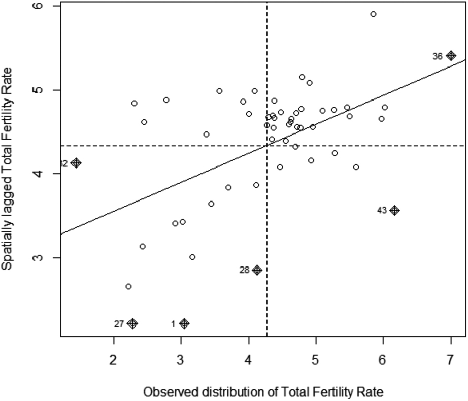
From Fig. 4 it can be seen that the observations have a particular spatial structure and the linear regression slope is non-null indicating a correlation between TFR and its spatially lagged values. The regression line shows a positive relationship (its slope is defined by the value of the value of Moran’s I given in Table 4 as 0.345) and most of the observations are in the upper right corner of the plot, indicating values of the TFR that are higher than the mean value (high-high). The lower left corner which has observations values lower than the mean (low-low) has the second highest numbers of observations after the upper right corner, followed by the top left (low-high) and lastly by the bottom right (high-low) corners in that order. The implication of this structure is that most countries with higher TFRs have positive spatial autocorrelation and high index value. Other countries are surrounded a mix of countries with high and low TFRs. There are six observations that do not follow the spatial structure as can be seen in the Moran’s diagram.
Figure 5.
Map of local moran index (iw) for spatial autocorrelation of total fertility rate at each location.
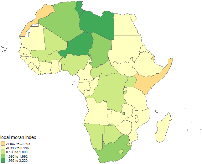
A local Moran output in Fig. 5 explores the local spatial autocorrelation and shows the intensity and significance of local autocorrelation between TFR value in a location and its value in the surrounding locations. Significant groupings of similar TFR values (positive local Moran statistic (Ii) values) can be seen around Western, Northern, parts of Middle and Southern Africa. While groupings of dissimilar values (negative local Moran statistic (Ii) values) can be observed mostly in Eastern Africa and Northern Africa and some countries around the coastlines.
From the map it is possible to observe the variations in autocorrelation across space. It can be interpreted that there seems to be a geographic pattern to the autocorrelation. In large sample observations, it may not be possible to understand if groupings are of high or low values. To obtain the local spatial autocorrelation structure for a more clearer picture, a map of the
Figure 6.
Map of
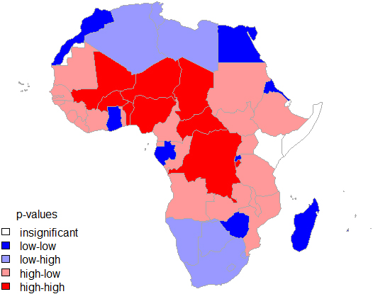
From Fig. 6, it is apparent that there is a statistically significant geographic pattern to the grouping of TFR across Africa. High-high locations have positive spatial autocorrelation and high index value, that is, a country with high TFR value is surrounded by countries with high values. Low-low locations have positive space autocorrelation and low index value. High-low locations have negative spatial autocorrelation and high index value. Low-high locations have negative spatial autocorrelation and low index value.
Since there is global spatial autocorrelation, the local Moran statistic of spatial autocorrelation shows that the areas with high-high local autocorrelation patterns are the ones with strong influence on the overall total fertility rate in Africa. It can also be seen that the distribution of local Moran’s I is centred on the global Moran’s I (Fig. 7). These zones have a significantly similar spatial association structure with the global structure and from Fig. 6, it can be seen that it is the region made up of countries with high-high local autocorrelations. From this it can be seen that the hypothesis of independence of observations does not hold as a result of spatial autocorrelation, hence analysis of the data with the usual statistical techniques may not be sufficient, thus the need of GWR technique that puts into consideration the influence of space in the dynamics of the total fertility rate is highlighted.
Figure 7.
Density plot of local moran index for total fertility rate (2017 data) in Africa.
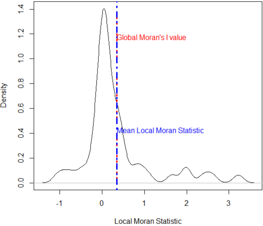
Table 5
Linear regression estimates
| Coefficients | Estimate | Std. error | ||
|---|---|---|---|---|
| Intercept | 4.35700 | 1.77300 | 2.457 | 0.01802 |
| Life expectancy at birth | 0.69399 | |||
| GDP per capita | 0.00004 | 0.01361 | ||
| Infant mortality rate | 1.086 | 0.28333 | ||
| % Contraceptive prevalence rate | 0.04144 | |||
| Unmet need for family planning | 0.405 | 0.68739 | ||
| Use of modern family planning | 1.042 | 0.30311 | ||
| Adolescent fertility rate | 0.01087 | 0.00295 | 3.678 | 0.00064 |
| Female labour force participation | 0.62358 |
Table 6
Linear regression estimates for best model
| Coefficients | Estimate | Std. error | ||
|---|---|---|---|---|
| Intercept | 4.07219 | 0.38184 | 10.665 | 2.95 |
| GDP per capita | 0.00003 | 0.00674 | ||
| Infant mortality rate | 0.00532 | 0.00504 | 1.056 | 0.29631 |
| % Contraceptive prevalence rate (CPR) | 0.00497 | 2.98 | ||
| Adolescent fertility rate | 0.01133 | 0.00245 | 4.635 | 2.76 |
The study continues with the analysis of the dataset on total fertility rate with respect to its determinants using the GWR, but first examines the results of ordinary least square (OLS) regression before looking at the GWR results and compares it with that of OLS regression, and lastly examines the GWR model fit.
3.2Analysis with GWR
Firstly, an ordinary least square (OLS) regression model was fitted for TFR given the predictors as displayed in Table 5. This shows that the variables in the model explain 72.6 percent of the variations in TFR (adjusted R-squared value 0.726). Of the factors considered in the regression only GDP per capita, CPR and AFR were the significant in the model. But it is known that unmet need for family planning and modern family planning have strong correlations with CPR, so one can be safe to say that this correlation was reflected in the model by leaving these two factors out.
It is worthnoting that female labour force participation, life expectancy at birth and IMR were not significant. To be sure of the result, several other models were fitted with different combinations of all the predictors to see how each fair comparing them with their adjusted R-squared values and AIC values. AIC takes in account the number of independent variables in each model and the maximum likelihood of the models, but penalises models with more parameters. According to AIC, the best-fit model (models with lower AIC scores) explains the greatest amount of variation using the fewest possible independent variables. Models with higher adjusted R-squared values and lower AIC values are preferred and selected among groups of models. The model given in Table 6 was found to be the best having adjusted R-squared value of 0.739 and AIC of 99.90. This means that this model has the fewest number of independent variables which account for 73.9% of the variations in TFR.
3.3GWR model coefficients
GWR was applied for the identified variables from the OLS model in Table 6 to take into account the influence of location on TFR as it fits different model at each point of the space. The output of interest here included a summary of the regression coefficient estimates across the Africa and a number of attributes which corresponded with each unique output area such as local R-squared and residuals. With AIC of 90.4 and Quasi-global R-squared value of 0.777 based on the GWR, these variables explained 77.7% variation in TFR.
Table 7
GWR model estimates
| GWR coefficients | Minimum | 1st quartile | Median | 3rd quartile | Maximum | Global |
|---|---|---|---|---|---|---|
| Intercept | 3.9219 | 3.9829 | 4.0323 | 4.0770 | 4.1222 | 4.0722 |
| GDP per capita | ||||||
| Infant mortality rate | 0.0037352 | 0.0040681 | 0.0064198 | 0.0074871 | 0.0080967 | 0.0053 |
| % CPR | ||||||
| Adolescent fertility rate | 0.010340 | 0.010765 | 0.011360 | 0.011545 | 0.012349 | 0.0113 |
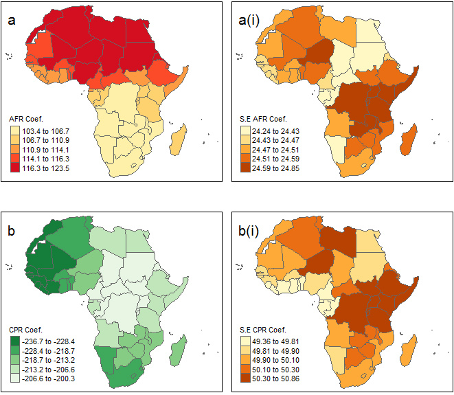
Figure 8.
Map of variable coefficients and coefficient standard errors (a) the plot of coefficients of adolescent fertility rate across Africa (a(i)) the plot coefficients standard errors for adolescent fertility rate across Africa (b) the plot of coefficients of percentage of contraceptive prevalence rate across Africa (b(i)) the plot coefficients standard errors for percentage of contraceptive prevalence rate across Africa.
The output from the GWR model in Table 7 reveals how the coefficients vary across the 53 countries. The global coefficients are exactly the same as the coefficients in the earlier OLS model. In this particular model, multiplying the coefficients by 10000 it can be seen that GDP per capita range from a minimum value of
The coefficients for IMR and ADR are positive with TFR. As IMR rises by 1 point for half of the countries in the dataset, TFR will increase between 40.681 and 74.871. Similarly, a unit change in AFR results in an increase in TFR between a minimum of 103.40 and a maximum of 123.49.
Table 8
Model comparison
| Model | AIC | Adjusted R-squared | Residual sum of squares |
|---|---|---|---|
| OLS | 99.903 | 0.739 | 16.297 |
| GWR | 90.387 | 0.777 | 15.095 |
Table 8 shows a comparison of the measures of model fit for GWR and OLS models and one can assess the benefits of moving from a global model (OLS) to a local regression model (GWR) as is evident in the measures’ values.
The distribution across space of the coefficients and their standard errors can be visualized as shown in the plots of GWR coefficients in Figs 8 and 9 for all the variables and are suggestive of spatial patterning.
Figure 9.
Map of coefficients and coefficient standard errors (c) the plot of coefficients of infant mortality rate across Africa (c(i)) the plot coefficients standard errors for infant mortality rate across Africa (d) the plot of coefficients of gross domestic product per capita across Africa (d(i)) the plot coefficients standard errors for gross domestic product per capita across Africa.
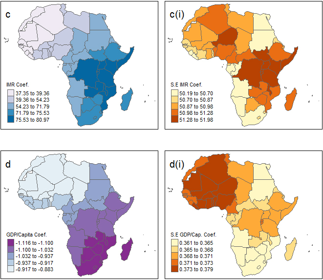
Looking at Fig. 8a plot, the coefficients for adolescent fertility rate can be seen to be highest in Northern Africa and some part of Western Africa (Mali, Niger and Nigeria), including Chad (Middle Africa) and Eritrea (Eastern Africa). The coefficients for adolescent fertility rate are lower in the other parts of Africa. Yet all across Africa, adolescent fertility rate has a positive relationship with total fertility rate. The CPR in Fig. 9c, the lowest coefficients are seen across Western Africa (Cote d’Ivoire, Liberia, Guinea, Sierra Loene, Guniea-Bissua, The Gambia, Senegal, Mali, Cabo Verde and Mauritania), including Morocco (Northern Africa). The highest CPR coefficients are seen in Middle and Western, while Southern Africa has lower coefficient compared to other regions.
From Fig. 9e plot, the coefficients for IMR is seen to be highest around Eastern Africa including Democratic Republic of the Congo (Middle Africa) and these values reduces as the circumference expands towards other part of Africa, with the least coefficients in parts of Western (Liberia, Guinea, Sierra Leone, Guinea-Bissau, The Gambia, Senegal, Mali, Cape Verde and Mauritania) and Northern Africa (Morocco and Algeria). Yet all across Africa, as IMR has a positive relationship with TFR.
Taking the Fig. 9g plot, which is for the GDP per capita coefficients, the spatial pattern is quite interesting. As can be seen from the plot, the lowest negative coefficient for GDP per capita is around Southern Africa and some parts of Eastern Africa and the values increases north-wards with the negative-maximum values seen in Northern countries of Libya, Tunisia, Algeria and Morocco, including Western countries of Benin, Niger, Burkina Faso, Mali, Senegal and Mauritania, plus Chad (Middle Africa).
Figure 10.
Map of GWR residuals.
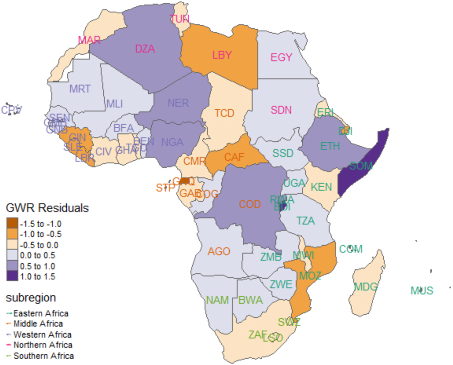
3.4Assessing GWR model fit
The residuals are examined to assess model fit and residuals above or below zero indicate that the model under- or over-predicts total fertility rate. The Residuals are mapped as shown in Fig. 10. It is expected that the grouping of negative and positive residuals would be randomly distributed. From Fig. 10, it can be seen that the negative and positive residuals are distributed across Africa.
Figure 11.
Histogram of GWR residuals.
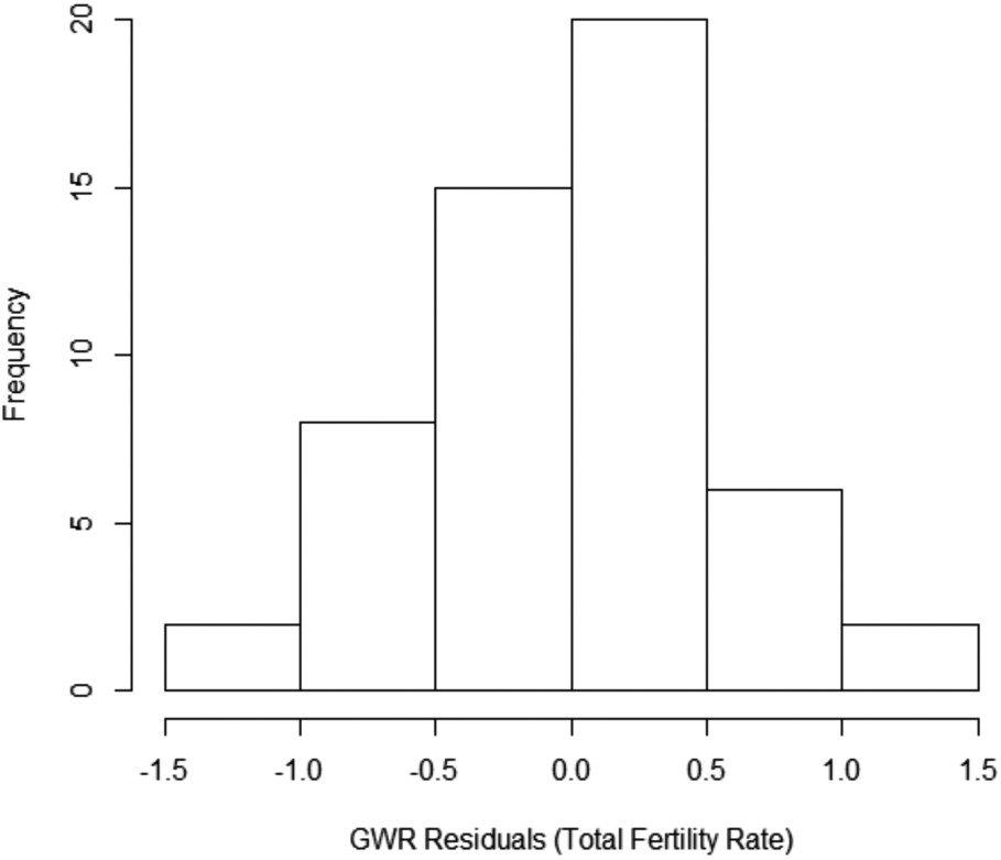
A histogram of the residuals in Fig. 11 shows the values are centered on zero and approximates a normal distribution across Africa.
Taking as threshold interval for residual (
Table 9
Countries with (over-predictions) below zero residual values
| Name | Residuals | Prediction | Prediction SE |
|---|---|---|---|
| Cape verde | 3.376 | 0.1582 | |
| Equatorial guinea | 5.613 | 0.2249 | |
| Sierra leone | 5.252 | 0.1764 | |
| Djibouti | 3.541 | 0.2107 | |
| Libya | 2.963 | 0.2000 | |
| Central africa republic | 5.437 | 0.2046 | |
| Mozambique | 5.529 | 0.1425 | |
| Guinea | 5.342 | 0.1504 | |
| Mauritius | 1.979 | 0.2970 | |
| Liberia | 4.894 | 0.2126 | |
| Madagascar | 4.628 | 0.1634 |
Table 10
Countries with (under-predictions) above zero residual values
| Name | Residuals | Prediction | Prediction SE |
|---|---|---|---|
| Rwanda | 0.5497 | 3.538 | 0.1784 |
| Algeria | 0.6024 | 2.443 | 0.1834 |
| Democratic republic | 0.6815 | 5.335 | 0.1423 |
| of the congo | |||
| Nigeria | 0.6845 | 4.772 | 0.1549 |
| Niger | 0.8172 | 6.183 | 0.2107 |
| Ethiopia | 0.9838 | 3.366 | 0.1956 |
| Somalia | 1.2166 | 4.951 | 0.1338 |
| Burundi | 1.3821 | 4.119 | 0.1434 |
Figure 12.
Map showing locations of over-predictions and under-predictions of total fertility rate.
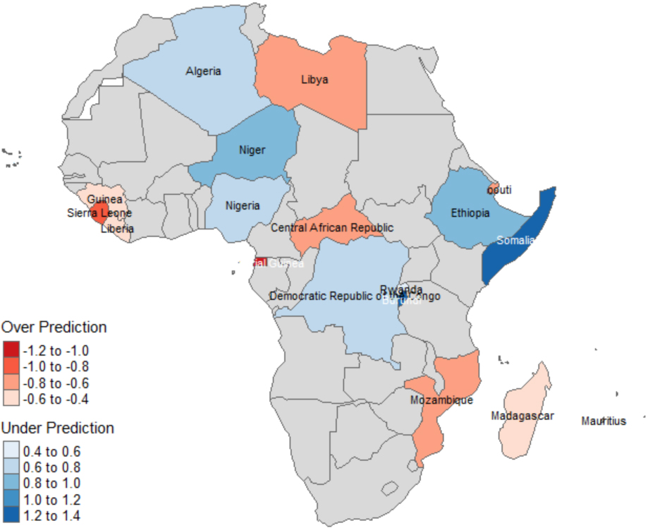
Figure 12 gives a pictorial overview of Tables 9 and 10 and it shows the map of Africa with the locations where the GWR over predictions and under predictions of TFR and also shows that they are random across space.
A Moran’s I Spatial Autocorrelation is run on the GWR residuals to confirm they are spatially random. The Moran’s I test shows that the residuals are significantly random with a
Table 11
Variables correlation matrix
| Moran I test under randomisation | ||
|---|---|---|
| Moran I statistic standard deviate | ||
| sample estimates: | ||
| Moran I statistic | Expectation | Variance |
| 0.036825519 | 0.008966225 | |
Figure 13.
Moran’s diagram for plot of GWR residuals against spatially lagged GWR residual values.
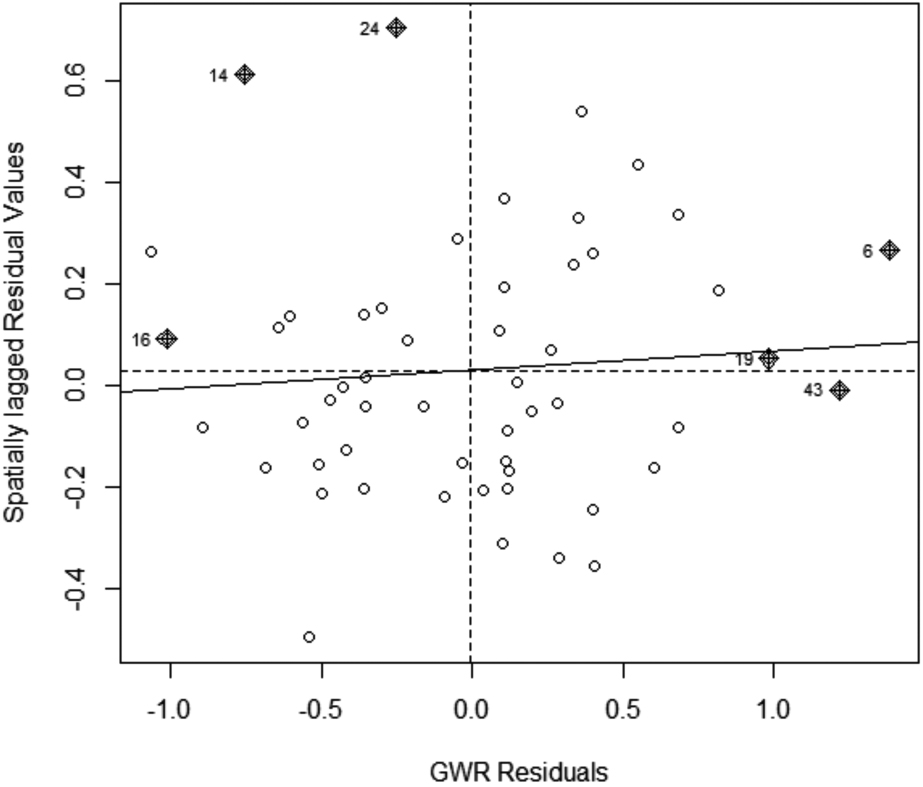
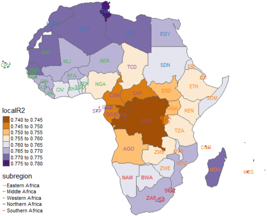
Figure 14.
Map of local R-squared values across Africa.
The Moran’s diagram in Fig. 13 shows a random distribution of the points on the plot of the GWR residuals against their spatially lagged values, which supports the Moran’s I test that there is no spatial autocorrelation of the residuals. The points are almost evenly distributed in each quadrant of the diagram and the regression line close to zero (horizontal to the x-axis) and the slope of the regression line is close to zero (0.036).
Figure 14 shows the map of the local R-squared values with the minimum and the maximum local R-squared values being 0.743 and 0.776 respectively at Democratic Republic of the Congo and Tunisia respectively. The minimum local R-squared value of 0.744 is above the R-squared value from the OLS regression; hence in this case, the geographical location in the evaluation in GWR improves the model’s ability to explain variability in TFR across Africa.
The map of the Local R-squared values also shows the locations where GWR predicts the best with highest values. GWR predicts well across Africa and shows that the predictor variables sufficiently explain the variability in TFR across Africa. They inherently capture many other difficult-to-track factors like religion and cultural practices.
4.Conclusion
Examining Total Fertility Rate (TFR) in Africa and the influence of its determinants in a spatial analysis framework is important to show how it varies across space and the resulting effect that may otherwise not be obvious without the consideration of geographical location in the analysis of datasets from the same. A couple of quantifiable determinants were taken as predictors to see their influence on TFR and how this influence varies across Africa. Spatial autocorrelation and geographical weighted regression analyses were applied on dataset for the period of 2017 that comprised observations from 53 African countries.
There was a statistically significant geographic pattern to the grouping based on a positive autocorrelation of TFR. Most countries with high TFR values were surrounded by countries with high values and a couple countries with low TFR values were around locations with low values. Fewer countries with high or low values were around those with high or low values. The positive global autocorrelation was majorly impacted by countries with high total fertility rates that were surrounded by others with high values too as reported by the local autocorrelation Moran statistic. These were countries bordering one another in Middle Africa up to Western Africa, which included Burundi, Democratic Republic of the Congo, Central African Republic, Chad, Nigeria, Niger, Benin, Burkina Faso and Mali.
The best OLS regression model showed that the statistically significant factors influencing total fertility rate were gross domestic product per capita, percentage of contraceptive usage and adolescent fertility rate. The latter two factors had significant correlations with unmet need for family planning and modern family planning methods. The GWR model was fit for total fertility rate with the identified significant factors from OLS model and GWR was better than linear regression as reported by the AIC, adjusted R-squared value and residual sum of squares values from both models. The AIC, adjusted R-squared value and residual sum of squares from GWR were 90.387, 0.777 and 15.095 respectively and those of OLS regression model with values 99.903, 0.739 and 16.297 respectively. The largest over-predictions of TFR from GWR model occurred at Cape Verde, Guinea, Liberia, Sierra Leone (Western Africa), Mauritius, Mozambique, Djibouti (Eastern Africa), Equatorial Guinea, Central Africa Republic (Middle Africa) and Libya (Northern Africa) while the lowest under-predictions occurred at Nigeria, Niger (Western Africa), Somalia, Burundi, Rwanda, Ethiopia (Eastern Africa), Democratic Republic of the Congo (Middle Africa) and Algeria (Northern Africa). The minimum local R-squared value of 0.744 from GWR was above the adjusted R-squared value from the OLS regression (0.739); hence geographical location as an influence on TFR across Africa which was included in the evaluation with GWR improved the model’s ability to explain variability in TFR across Africa.
Hence GWR predicted well across Africa and showed that the predictor variables sufficiently explain the variability in TFR across locations in Africa. The significant variables of GDP per capita, CPR and AFR inherently captured any other difficult-to-track factors that would influence TFR across Africa like religion and cultural practices.
The goal of Africa having to control its population for economic, infrastructural and developmental planning and policy making is realizable if focus on controlling fertility rate can be placed in countries around Middle Africa up to Western Africa, that have been identified in this study to be those that significantly affect the overall TFR in Africa. The governments of these countries can also be advised on programmes to help educate their populations on the effect of large households in the present economic realities and the effects of climate change on the continent. More intense works should be carried out in these countries to see how the underlying factors that affect CPR and AFR can be properly managed so that fertility rate in Africa can be reduced and hence help deal with the challenges of overpopulation in Africa.
Acknowledgments
World Bank Open Data source.
United Nations, Department of Economic and Social Affairs, Population Division.
The Demographic and Health Surveys (DHS) Program.
References
[1] | Opiyo C. Fertility levels, trends and differentials. Kenya Demographic and Health Survey. (2003) ; 4: : 51–62. |
[2] | Mberu BU, Reed HE. Understanding subgroup fertility differentials in nigeria. Popul Rev. (2014) ; 53: (2): 23–46. doi: 10.1353/prv.2014.0006. |
[3] | Sneeringer SE. Fertility Transition in Sub-Saharan Africa: A Comparative Analysis of Cohort Trends in 30 Countries. DHS Comparative Reports No. 23. Calverton, Maryland, USA: ICF Macro. (2009) . |
[4] | Westoff CF, Kristin B, Dawn K. Indicators of Trends in Fertility in Sub-Saharan Africa. DHS Analytical Studies No. 34. Calverton, Maryland, USA: ICF International. (2013) . |
[5] | Bongaarts J, Casterline J. “Fertility Transition: Is Sub-Saharan Africa Different?” In Population and Public Policy: Essays in Honor of Paul Demeny, edited by G. McNicoll, J. Bongaarts, and E.P. Churchill. New York, New York, USA: Population Council; (2013) . |
[6] | Matthews SA, Parker DM. Progress in spatial demography. Demographic Research. (2013) ; 28: (10): 271–312. doi: 10.4054/DemRes.2013.28.10. |
[7] | Brunsdon CA, Stewart F, Martin EC. Geographically weighted regression: a method for exploring spatial nonstationarity. Geographical Analysis. (1996) ; 28: (4): 281–298. |
[8] | de Bellefon M, Floch J. Geographically Weighted Regression. Handbook of Spatial Analysis. Theory and Application with R. INSEE Eurostat; (2018) . |
[9] | World Bank Open Data 2019 [cited Nov 2019]. Available from: http://data.worldbank.org. |
[10] | United Nations, Department of Economic and Social Affairs, Population Division. World Family Planning 2017 – Highlights (ST/ESA/SER.A/414). |
[11] | Salima BA, de Bellefon M. Spatial Autocorrelation Indices. Handbook of Spatial Analysis. Theory and Application with R. INSEE Eurostat; (2018) . |
[12] | Upton, Graham, Bernard Fingleton, et al. Spatial data analysis by example. Volume 1: Point pattern and quantitative data. John W & Sons Ltd, (1985) . |
[13] | Fotheringham AS, Brunsdon C, Charlton ME. Geographically Weighted Regression: The Analysis of Spatially Varying Relationships. Wiley, Chichester. (2002) . |
[14] | Bivand R, Yu D, Nakaya T, Garcia-Lopez M-A. spgwr: Geographically Weighted Regression; (2017) . Available from: https://cran.r-ptoject.org/package=spgwr. |
[15] | Bongaarts J. A framework for analyzing the proximate determinants of fertility. Population and Development Review. (1978) ; 4: (1): 501–132. doi: 10.2307/1972149. |


