
Exploring the use of earth observation and data science for agricultural statistics to complement the census dataset: Case study for Namibia Statistics Agency
Abstract
Agriculture is the backbone of human life, it enables for food security, health and economy. Yet, many countries in Africa suffer from poor accessibility to agriculture data which is crucial for policy makers and farmers. Half of Namibia’s population depend on agricultural activities, for as their main income source, much of which is undertaken on smallholdings. Therefore, compiling statistics around agricultural outputs is of primary concern to many national statistics agencies Unfortunately, challenges to account for agriculture crop production statistics include low frequency of data collection, lengthy data processing periods, and the lack of timely output which can be linked to policies and decision making. This paper explores the use of satellite imagery and data science techniques in a statistics agency to complement the agriculture census. The paper assessed Google Earth Engine for image processing and extracted a range of indices (NDVI, SAVI, MSAVI and GLCM and Tasseled Cap Index based) in order to identify smallholder farmers’ plots and estimate the field area in a rural village in Namibia. Although groundtruth data was not available at the time of this issue, the findings showed a promising starting point for a scaled project.
1.Introduction
Agriculture and food security systems face many challenges and environmental issues as a result of climate change. National statistics offices (NSOs) are under pressure more than ever to produce real time, high quality and relevant statistics. With the launch of the Sustainable Development Goals (SDGs), Namibia along with other nations, has joined the quest to end hunger and poverty by 2030, this is a big commitment, especially for developing countries that have less and limited capacity to monitor progress toward these targets and analyse the underlying causes of observed trends [1]. Namibia’s first Sustainable Development Goals (SDGs) Baseline Report launched in 2019 [2] revealed that Goal 2, indicators linked to proportion of agricultural area under productive and sustainable agriculture, was not reported as there were no sources of data identified. The people most affected by this goal are smallholder farmers, who depend on agricultural crop production for nutrition and as the main household income. Smallholder farmers make up 50 percent of the rural population in the northern regions of the country [3]. Agricultural and rural statistics are compounded by the low frequency of data collection, lengthy data processing time and the lack of timely output to link to policies and decision making. NSOs are under pressure to collect data at reduced cost and resourcing whilst still ensuring timely and high quality of statistics are produced. In the data revolution era, some statistics offices have adopted the use of big data and satellite imagery, however this is a case mostly found in the developed nations. Traditionally, these technologies have required specialist capabilities and sophisticated storage to handle their data and undertake analyses. But, in recent years there has been a growth in platforms that open up their potential to data scientists and analysts. One such platform is the Google Earth Engine (GEE), which provides access to petabytes of global imagery on Google’s Cloud architecture, using conventional remote sensing and data science approaches. NSOs can tap into these opportunities too. This paper explores the use of satellite images to detect agriculture plots and estimate the crop land use area in order to highlight and recommend changes required for the existing data collection systems.
2.Problem statement
Namibia is considered to be the driest country in the south of Sub Saharan Africa, the productive agricultural land lying mostly between two deserts, the Namib Desert in the West and the semi-arid Kalahari Desert in the South East.
The total land area reported to be viable for agricultural activities is estimated around 388 200 km
As a recommendation from the international development organisations such as the FAO, World Bank, a country should carry out a national agriculture census every ten years, which should be complemented by annual surveys on few selected topics. However, Namibia has conducted only three Censuses in the past 30 years since Independence. As a result, agricultural and rural statistics in Namibia are weak and hampered by huge data gaps and most key indicators are imputed from outdated sources [4].
Earth observation data and tools can be used to fill data gaps in NSOs. Remote sensing and data science have gained a prominent reputation in recent years as regards to producing statistics and monitoring measures for countries, especially the developed world. This paper explores the use of satellite imagery and data science to complement traditional data collection methods. Due to the challenges in obtaining ground truth data, this paper aims to demonstrate a practical pipeline in effort to extract statistics for agriculture. The paper aims to answer the following questions;
1. The type of information that can be obtained from satellite imagery at different resolutions
2. What type of techniques or methods can be developed to extract this information?
3. Can the area of smallholder plots be calculated accurately from the satellite imagery?
4. What ground truth data, and its sample size, is required to build a model?
3.Remote sensing and Earth observation data
Remote sensing is the techniques of science and technology that observe and record earthly objects from pace with instrument-based techniques like sensors. Satellite imagery captures information through passive or active sensors, which receive reflected or radiated electromagnetic (EM) waves from objects. The amount and characteristics of the electromagnetic radiation and reflectance depends on the type and condition of the Earth object. The human eye can see only a portion of the spectrum of visible light; red, green and blue. Other wavelengths such as long-range infrared and short are not visible to the human eye but can be usefully detected by satellite sensors.
In relation to vegetation, we can discriminate between vegetation types and their state of health by studying infrared (IR) and visible red light. During photosynthesis, the plant absorbs visible red and reflects near-infrared (NIR). Because this relationship between these two bands changes between healthy and diseased or dying (sensing) plants, when less visible light is absorbed by chlorophyll, they are used extensively for vegetation monitoring. For example, the Normalised Difference Vegetation Index (NDVI) is calculated as the ratio between measured canopy reflectance in the red and near-infrared bands and ranges always between
NDVI is widely used in remote sensing to monitor global vegetation cover and biomass. Other uses include drought monitoring, crop classification, and measuring of production. NDVI has been used successfully in analysing the vegetation, but is known to be sensitive to atmospheric, soil color, cloud shadow and the effect of leaf canopy [6]. To address some of these concerns, the Soil Adjustment Vegetation Index (SAVI) was developed to improve the soil background from the NDVI by minimizing the soil reflectance. This was achieved by incorporating soil conditioning correction factor; L [7]. The L factor has various ranges (0.25, 0.3, 0.4, 0.5), which are suitable for different soil types and the value 0.4 has been viewed as appropriate for the crop period [8]. Later, the Modified Soil Adjustment Vegetation Index (MSAVI) was created to reduce the influence of bare soil on SAVI [7]. Both MSAVI and SAVI value range between 1 and 0. Another index considered in this study was the Tasseled Cap Index based on a linear combination of bands.
4.Remote sensing tools and platforms
4.1Google Earth Engine (GEE)
Use of parallel computing and big data has merged intensively over the last decades due to the overflow in the availability of data [9, 10]. GEE is a platform that allows access to work with large amounts of data and is developed to allow large computing of planetary datasets using parallel processing. GEE is designed on top of a distributed system that shares resources and computing, which means the user does not need to have local capacity such as, additional infrastructure to handle large amounts of information on their computer. This is an advantage for users because they do not need local sophisticated computer ecosystems to perform tasks on Google Earth Engine. The engine itself is built on top of a collection of technologies that are found within the Google data center environment [9]. Cloud computing also makes it easier for users to share code and integrate their findings online from all over the world. This is beneficial as statistics offices can share resources and compare findings easily in the region or internationally.
In the case of developing countries in Africa particularly, there are huge constraints on the advanced computer infrastructures and storage space. Many countries cannot afford to have complex systems setup to support huge processing of the images [10]. The environment offers a new era of cheaper, quicker intervention tools to monitor across areas of global concerns such as vegetation, deforestation, water and land use [11]. Besides, GEE is a free platform, for non-commercial use, and considered easy to use with many consolidated libraries to make use of [12]. GEE has been used extensively in the areas of climate change, agriculture and weather conditions. However, in the area of crop mapping and yield estimate, a literature review indicates that few of these studies made use of GEE and very few are actually done in Africa [13].
4.2Remote sensing in agriculture
Images can be classified through unsupervised and supervised machine learning algorithms. In unsupervised learning, a user is not required to have training data beforehand. While in supervised learning, the user is expected to already have “known” homogenous training imagery of the different earth surface cover type of area of interest. In some cases, research combines supervised and unsupervised learning approaches to aim for better results [14]. Unsupervised learning is commonly used to first identify the largest segments of spectral classes and later, these used in a supervised learning approach for final results. Other methods of image classification are pixel-based classification. Each pixel will be assigned to one spectral class of spectral bands, used in the classification. These spectral classes will be linked to the surface attribute, such as crop land roads or water. Object-based classification, partition image pixel values into spectrally similar regions that can correspond or be assigned to the surface attributes, such as crop field, flood plain.
5.Methodology
In this paper, we are exploring the use of Google Earth Engine (GEE) and all image processing was done in GEE. Supervised and unsupervised was adopted in the study. The satellite imagery used in this assessment was Sentinel-2 imagery produced by European Commission and European Space Agency. Agriculture is one of the applications highly supported by this satellite mission which has high resolution for visible bands, at 10-meter pixels, and good temporal resolution.
After establishing the challenge of acquiring the groundtruth data, two separate methods were tested to detect the agricultural plots. The first was to identify the type of information required to distinguish the agricultural plots from other features using unsupervised classification. The second, used training and testing polygons that were digitised and applied to train supervised classifiers. Finally, imagery for farming areas was classified and the area of pixels assumed to represent fields/plots, as verified on a base map, was calculated by segmenting contiguous regions of pixels into polygons.
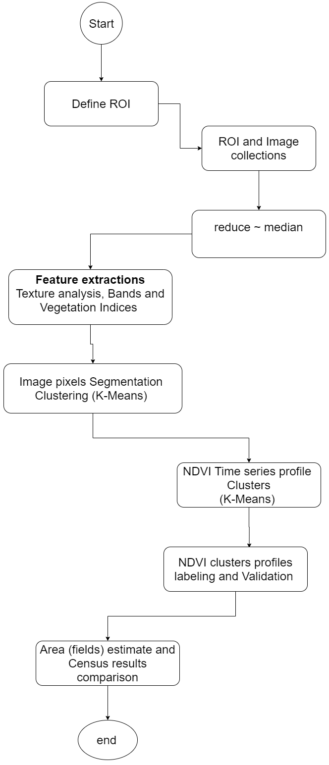
In order to identify an agricultural field from a non-agricultural field and calculate the plot area of the small farmer holders, we created a pipeline with three main steps for the pixel-by-pixel and unsupervised classification approach, which are; detecting the agricultural area, identifying and validation the plots and calculating the plot pixels area from imagery Fig. 1.
Figure 1.
Main steps in the pipeline.
5.1Ground truth data and region of interest (ROI)
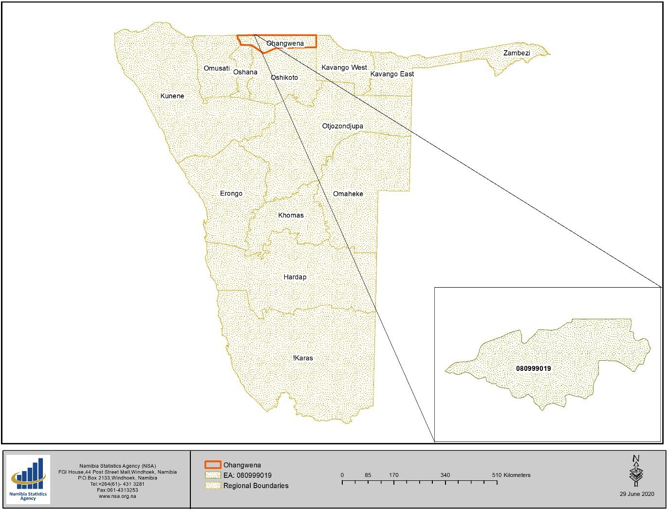
For the ground truth data, the initial idea was to use the agriculture Census 2013/14 dataset which included field coordinates points, polygons and other key variables to complement the findings from satellite imagery. During the data exploration process, it was discovered that the data was not fit to use and could not be used for validation as initially planned. Instead, a random primary sample unit (PSU) from the national sample frame, in the Ondobe constituency, Ohangwena Region was used for demonstration. From the agriculture Census 2013/14 data set, we extracted households’ data for this PSU and aggregated the total agriculture households and their area of planting. At least 73 percent of households practice crop farming in that area. Figure 2 shows the administrative boundaries and the region where the area of study is situated.
Figure 2.
A map of namibia regions and area under study (inserted image).
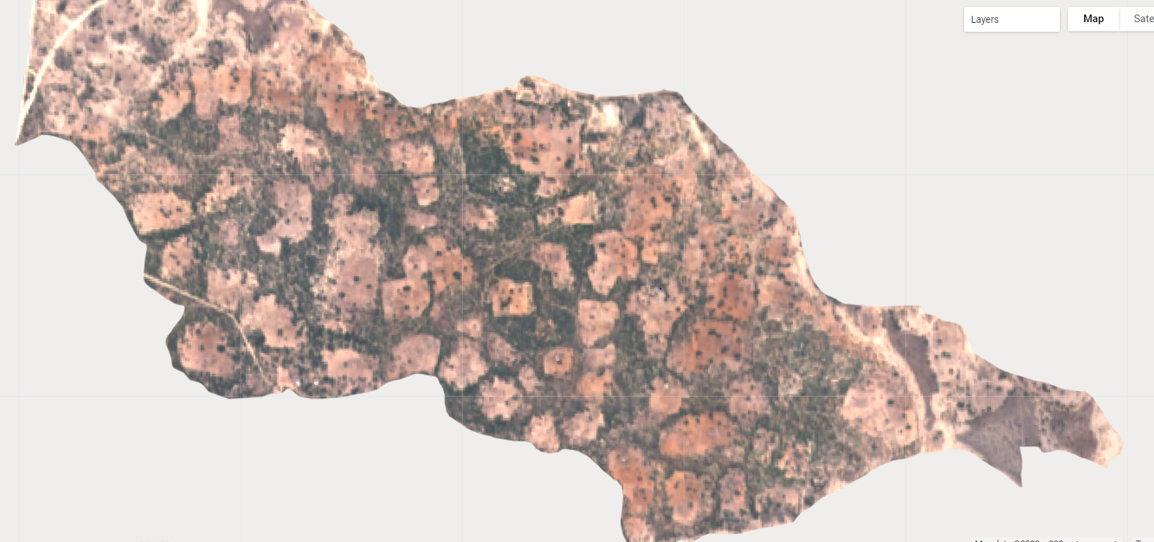
Millet is the primary staple crop in this area, while Sorghum is harvested in small amounts. The growing season lasts five to six months, January to May according to the historical data. The harvest season lasts from May to July. The paper follows the seasonal crop calendar to produce composite images. For the processing a median image was calculated from images gathered over the period of January 2016 to December 2016. This was so in order to extract images that are taken close to the Census 2013/14 data collection period since sentinel 2 imagery are only available from July 2015 Fig. 3 exhibit the sentinel 2 image of the region of interest (ROI).
Figure 3.
Sentinel Red, Green, Blue (RGB) image at 200 meter per pixel, of a rural village and visible fields, from March 2016.
5.2Image processing
Besides the region of interest, other aspects that we had to consider were the time of year, resolution, coverage, cloud cover and bands. Sentinel 2 captures images of 10 m resolution in the visible spectrum approximately every two weeks. Cloud cover and ground coverage can challenge the suitability of images for processing. Fortunately, sufficient cloud-free images were found during pre-analysis of the data.
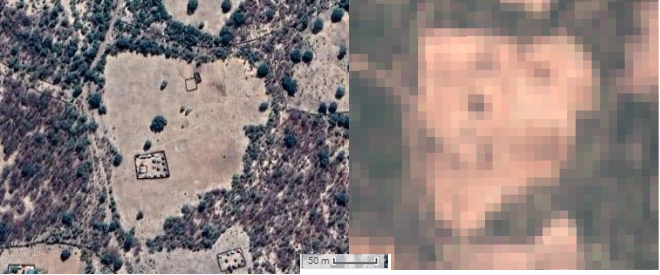
We took a year’s (January 2016 to December 2016) images, equivalent to one crop calendar, and calculated a composite image based on the median pixel value at location during this period, meaning it had the least cloud cover. The time of day images were captured was not considered a major criterion although this is important where groundtruth data is collected. From the images it was clear to distinguish the cleared area used for agriculture, what are called plots or “epya” in a native language of oshiwambo, from the surrounding area by the lack of vegetation over most time of the year. Figure 4 shows two images of a typical smallholder field, using a sentinel 2 true-color composite and the Google’s high-resolution base map imagery. The latter uses commercial imagery that is not available for processing in GEE, only visualisation.
Figure 4.
Two images, left showing a sentinel 2 true-color composite and right, the Google’s high-resolution base map imagery of plot and surroundings.
Since the paper is focused on small scale farming, the process to identify the small plots becomes a challenge, due to uneven land structures and non-fenced fields making it difficult to clearly distinguish contrasting land use and field boundaries [15]. In Namibia, small scaled farms are not demarcated by any physical distinguishable boundaries. The borders are often made by walking paths or by trees and shrubs. This makes ground truth data crucial in verifying the accuracy of a classification model. However, these fields are easily noted by their lack of vegetation and different texture as compared to the nearby land.
5.2.1Detecting agricultural fields from non-agricultural fields using unsupervised classifications
As established earlier, during image processing vegetation indices proved to be valuable in distinguishing a farmer’s plot. The indices derived from the Sentinel 2 images are the NDIV, MSAVI and tasseled cap greenness. These indices were derived for the dry season starting from June 2016 until December 2016 and for the rainy/growing season from January until May when the harvest season starts.
In addition, texture analysis was performed as the next step. This was done because there is a clear difference in the ‘texture’ of plots’ pixels and their surrounding areas, particularly with the NDVI and MSAVI values. The texture analysis was performed on a greyscale (single band) image derived from the RGB bands. To produce the greyscale value, the image RGB bands are changed to HSV (Hue, Saturation, Value) and the Value band (brightness) is extracted and used to calculate the Gray-Level Co-occurrence Matrix (GLCM) which is used to measure texture in a range of different ways [16].
Texture metrics such as entropy, homogeneity and contrast had promising contributions to the segmentation of the pixels during clustering. There is need to test further on different metrics with high resolution images less than 10 m and when the ground truth become available.
After extracting texture metrics and vegetation indexes, these bands were all added into one image, creating a 25-band image. Principal Components Analysis (PCA) was used to reduce the bands into few components based on the variability of pixel’s values across bands, refer to Fig. 5. The image output from this process was used as an input for the image segmentation by clustering (unsupervised classification) to identify the plots. We compiled a one-year time series of monthly NDVI found at each plot identified and exported these results for further modelling to identify similar plots and compare the results. The monthly NDVI time series profiles calculated for each of the segmented features were clustered to identify plots with similar growing profiles.
Figure 5.
Results of PCA component, showing the prominent features from the pixels reduced, there is some clearly visible degree of dissimilarly between the field pixels and surrounding neighbours.
5.2.2Area calculation
Once the NDVI profiles were clustered, the cluster with the NDVI profiles that showed most similarities to a typical crop phenological calendar were identified and analysed further including manually validating the accuracy against Google satellite base map imagery.
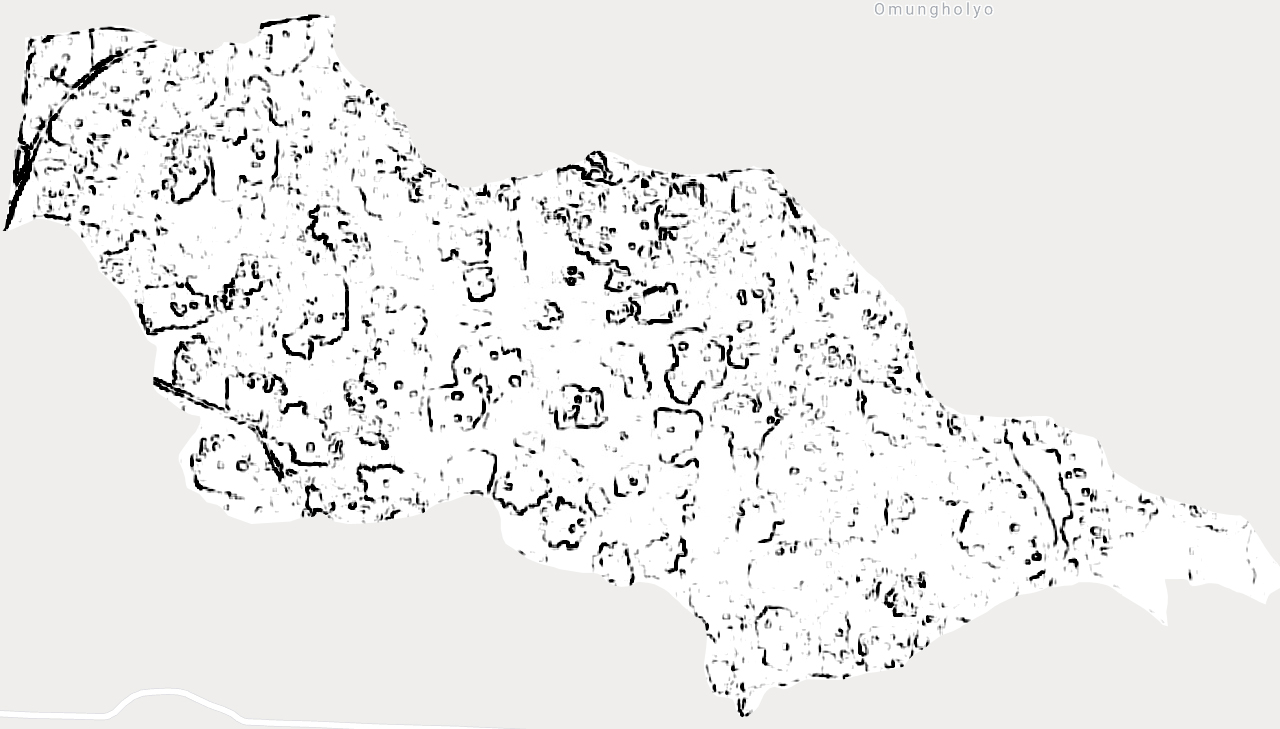
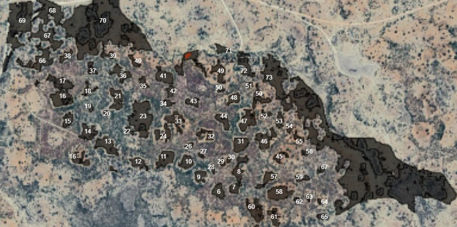
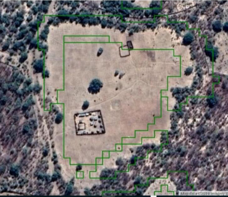
The area under these plots for the clusters identified was calculated and matched with the statistics recorded from the Census agriculture 2013/14. We manually assessed the validity of these patches obtained during the unsupervised classification; however, we cannot accurately pronounce them as crop field without ground truth, refer to Fig. 6.
Figure 6.
Image of the manual mapped and numbered features from the unsupervised classification process.
Some of the observations from the region of interest that could be found useful for the main study and for other NSOs considering earth observation datasets;
1. Fields are distinctive patches of open, less vegetation ground, especially in semi-arid areas
2. They are mostly misshaped and uneven with an average size around 2 ha
3. In the case of Namibia, some fields are attached to one another, hence it might be more practical to aggregate the statistics at a constituency level, for instance total area estimates.
5.2.3Supervised classification method with manual digitised polygons
The lack of ground truth data meant there was no surveyed training data for this process. In an attempt to test the classification models, digitised polygons were manually created for the study area grouping features into four land classes; plots, water (floodpans), and trees and shrubs/bushes. A total of 75 plots, 20 trees, 10 waterpans and 21 shrubs were produced making 126 elements for training. To create testing data, the area of interest was extended to promote diversity. A separate test data from the area surrounding the ROI was sampled against the classified dataset. These are the steps taken to create training and testing data using Google base map data.
• Digitised plots were created using the Google Earth base map imagery. Features were identified as plots based on the local knowledge of the area.
• All the visible plots in the study area were digitised. A total of 126 features were digitised into polygons for training.
Another set of features were digitised in the extended image to create validation data for the classifiers. Random forest and CART (Classification and regression) were both tested against the training data that was sampled from the image. To build the models, a median composite of Sentinel 2 images was used with seven bands plus the land cover class. A total number of 3030 pixels were sampled. The model was built from the Sentinel-2-pixel values found in the training polygons and then the accuracy tested using the pixels from a different area. A total of 969 pixels were sampled from the testing features manually digitalised.
Given ground truth data, there would be a need to assess various sampling strategies such as the stratified sampling to ensure true representative of the features and to strengthen the model prediction accuracy. In this study, sample region technique was used in creating the training and testing data, where each band becomes an additional property in the image.
6.Findings
Due to the lack of actual surveyed ground truth data, it was not possible to fully validate the information and whether the plots identified are a true reflection on the ground at the time of writing this paper. However, based on comparison to high resolution base map imagery the results obtained from both unsupervised and supervised classifications yield promising results and show potential pipeline improvement once the ground truth data are available.
6.1Detecting the agricultural small farmer
One of the challenges with detection of small farm holdings in Africa, is the uneven land type and the heterogeneous landscape found in these areas.
The preliminary results on Sentinel-2 true-color (red, green, blue) images indicate that plots are evidently distinguishable from the surrounding environment due to the level of the vegetation at different seasons. In summer there is a lack of vegetation as compared to the landscape around, such as the shrubs and trees were observed to have a consistent high vegetation.
Vegetation indices tested during the unsupervised classification were the NDVI, MSAVI and the Tasseled Cap Greenness. The indices were combined together with red, green, blue and near-infra-red for dry season and rainy season of the entire area of interest.
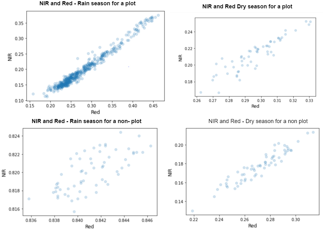
The RED and NIR extracted from the pixels inside the polygon of a plot for both dry season and rainy season, extracted in March 2016 and September respectively, show the correlation between these two bands and how they change over time, Fig. 7 shows the correlation between the NIR and Red bands for both rainy and dry season for a plot pixels and non-plot pixels.
Figure 7.
Correlation of NIR and RED for both rain and try season in a plot polygon for one annual crop calendar.
The Tasseled Cap Greenness was used instead of the other two dimensions of the index, the wetness was not considered here due to the dry savanna landscape of Namibia. However, during the model training with ground truth data, this dimension will be tested especially for the rainy season.
When the indices values of the MSAVI on both seasons are examined, the values for the plot’s areas during the dry season show more concentrated and high values as compared to the rainy season. This could be contributed to the fact that during the rainy season crops are growing on those plots and hence have a high NDVI compared to the MSAVI. As is true for the summer season, where the values of the NDVI decrease as compared to high MSAVI values. Figure 8 shows the difference in NDVI between summer (right image) and rainy seasons (left image).
Figure 8.
NDVI level at different times of the year. More concentration during the crop growing season (left) in Feb 2016 and less during dry season (right in August 2016.
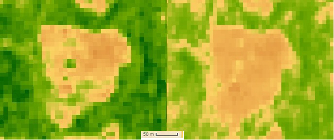
Figure 9.
Cluster zero – the NDVI times series profiles with a centroid (green line).
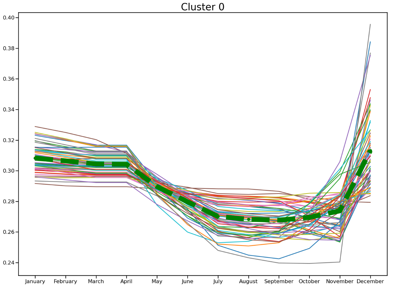
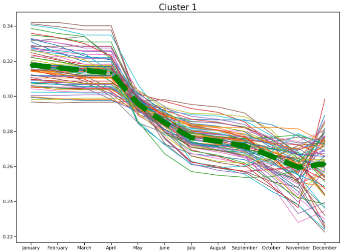
Figure 10.
Cluster one – the NDVI times series profiles with a centroid (green line).
The MSAVI ratio showed a high concentration during the summer/dry season, which is a valid considering that these fields are normally cleared after harvest to prepare for the next growing season. The statistics are significantly different between the pixels of the plot polygon and that of a non-plot.
Combined with indices, the texture measures can be used to further discriminate the area used for cropping from other areas. Texture measures derived from Sentinel-2 image, grey-level-co-occurrence matrix (GLCM) such as contrast, homogeneity and entropy proved to yield promising results in distinguishing the area of the plot as compared to the surrounding areas. However, this process is worth revisiting when the ground truth data becomes available.
The images were segmented through clustering and a total of 140 elements were discriminated according to neighbouring similarities. Upon investigation, it was discovered that some features overlap, especially where the fields have big trees and where the area is covered more by bare soil with less vegetations. It would be interesting to collect sample training data from various land topographies of the country and examine how the model will perform at similar time of the year.
Although the NDVI profiles for the year were clustered according to the similarities in the neighbouring pixels, there was a clear overlap of these features and further investigation is being undertaken on which other indices can be used to further segmentation.
6.2Clustering NDVI time series profiles
Crop activities for Namibia can be summarised into three main seasons, the planting and growing season, the harvesting season, and the dry season. The growing season for Namibia crop is January to May (FAO), with the observed weather changes recently the rainy season starts later in the year influencing the planting seasons and with the absence of an updated crop calendar.
Clusters labelled zero, Fig. 9 and Cluster one, Fig. 10 both demonstrate similar patterns in the phenological profiles of the feature included in these clusters.
Cluster two, Fig. 11 the NDVI profile on these pixels are relatively high throughout the season which could be contributed to the fact that these include trees that are active and green throughout the season.
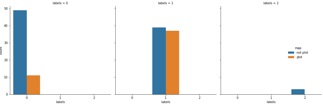
The Table 5 and Fig. 12 summarises the results obtained after clustering the NDVI profiles. Each cluster, the features were then labelled crop or non-crop after manual validation.
6.3Supervised classification method
In the absence of ground truth data to use for training the supervised model, different polygons were created for features such as the plots, trees, floodpan and shrubs/bushes.
Results from two models were obtained by training models against the training data inside the polygons of features mapped, from high resolution base map imagery, and then testing against independent pixels outside the training set which the model had not been exposed to.
The prediction given in Table 1 shows of the two models the random forest was more successful in classifying the validation pixels against the classification pixels. The random forest scored a 96% Kappa coefficient, demonstrating the level of accuracy in classifying the pixels compared to values assigned by chance, while the CART Kappa coefficient only reached 50% accuracy level.
Table 1
The result of the accuracy rate for random forest and CART model
| Model | Cart | Random forest |
|---|---|---|
| Overall accuracy % | 91 | 98.6 |
Table 2
Random forest confusion matrix
| Features | Plot | Tree | Water | Shrubs | Total |
|---|---|---|---|---|---|
| Plot | 862 | 3 | 8 | 30 | 903 |
| Tree | 2 | 9 | 0 | 24 | 35 |
| Water | 5 | 0 | 14 | 0 | 19 |
| Shrubs | 4 | 0 | 0 | 8 | 12 |
| Total | 873 | 12 | 22 | 62 | 969 |
Table 3
CART confusion matrix
| Features | Plot | Tree | Water | Shrubs | Total |
|---|---|---|---|---|---|
| Plot | 856 | 5 | 14 | 28 | 903 |
| Tree | 5 | 6 | 0 | 24 | 35 |
| Water | 5 | 0 | 13 | 1 | 19 |
| Shrubs | 5 | 0 | 0 | 7 | 12 |
| Total | 871 | 11 | 27 | 60 | 969 |
A confusion matrix is a method of comparing the ground truth data to the predicted value, identifying the classification errors and their associated quantities.
The results summarised in the confusion matrix shows both models, Tables 2 and 3 appear to predict the plot pixels well from the classified image, both pre-dicted at least 80% of the plots pixels the same as the
Figure 11.
Cluster two – the NDVI times series profiles with a centroid (red line).
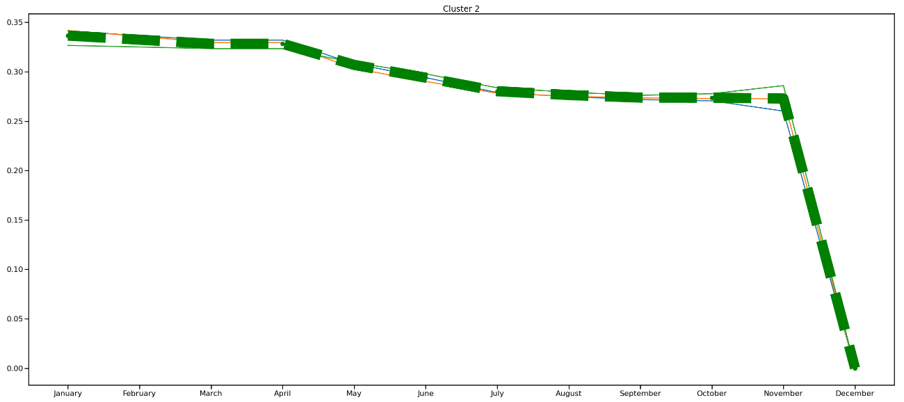
Figure 12.
Results of the unsupervised NDVI profile clustering method, clusters labelled plot and non-plot after manual validation.
classification. With the CART model, a 3% of the plot pixels in the validation data were classified as shrubs or bushes in the classified image. This among other factors, could be contributed by the fact that some field pixels are potentially overlapping with tree pixels because most of the fields in the study have big trees. Figure 4 shows a true-color composite image of a plot and trees clearly distinguishable from the features.
As part of improving the model, masking over prominent features in the northern region of the country where most small holders reside will improve the classifier’s accuracy. Features such as floodpans, which build up water during the rainy season, and trees can be masked by defining an appropriate NDVI threshold. Although there was no groundtruth data, results show that none of the models classified the pixels labelled water as trees or shrubs.
Once the groundtruth is available its other models such as SVM and neural networks can be tested and validated.
6.4Calculating areas
Using the agriculture Census, we filtered the dataset to the area of study and aggregated the area under crop production; the estimated figures 53.7675 Ha (without the weight). The total number of plots interviewed during the census was 85 and households that indicated practice of agriculture activities were 81 – this however included livestock, 50% of these practiced crop farming.
To calculate the area, Sentinel 2 pixels with an NDVI profile similar to crops were manually verified against Google’s base map and the area calculated from inside segmented polygons converted to hectares. The total area of plots was a combination of correct plots pixels from cluster zero and one where the feature plots were found. A total of 48 plots were identified from the segmented area, however this means that some of the true positive features were missed as seen in Table 5. The difference in the total plots could also be attributed to the fact that some of the identified plots contain multiple census plots, however we would not be able to determine the internal boundaries, Table 4 and shows the difference area sizes between the census file and Table 6 shows the calculated area from the satellite imagery.
Table 4
Agriculture census 2014/15 datasets showing area plot estimate by farmer and the actual plot measurements by interviewers
| Data source | Total area |
|---|---|
| Census farmer’s estimate | 58.39 Ha |
| Area census measurement | 53.7675 Ha |
Table 5
Results of the NDVI profile from the clustering technique, clusters are labelled plot and non-plot
| Features | Cluster zero | Cluster one | Cluster two |
|---|---|---|---|
| Plots | 11 | 37 | 0 |
| Not plots (trees, shrubs and | 38 | 39 | 3 |
| waterpans) |
Table 6
Area calculated from the sentinel 2 imagery; segmented features obtained during the clustering method
| Cluster | Total area of field patches pixels |
|---|---|
| Cluster one | 67.05613 |
| Cluster two | 0 |
| Cluster zero | 26.42179 |
6.5Validation
The final step in this paper was validation. Model validation is crucial to assess the accuracy of the model against ground truth data. The confusion matrix summarizes the performance of a classification algorithm. Tables 2 and 3 show the confusion matrix of the two-modelling output.
For the unsupervised classification, the clusters that exhibited similar NDVI trends to a crop were taken into a further rigorous manual exercise where the Google base map was used to validate the features in the clusters.
The total areas of the features that were seen as plots and had an NDVI profile corresponding to the phenological sequence of the crop seasons was compared to data from the agricultural census. The data from the census file was aggregated to the primary area unit related to the study area, and the estimated figures from the farmers and the field measurements from the interviewers obtained shown in Table 4. To validate the plot areas, the total area of the clusters exhibiting the acceptable NDVI profile were aggregated. Table 6 summarises the area estimates based on the Sentinel 2 imagery.
Comparing the total areas between the Sentinel-2 data and the census dataset, even given the limited amount of ground truth data, yields a good correlation. The differences in values can be attributed to various points. For the Sentinel-2 data, the issues of the scale and time of image acquisition can influence a great deal, Fig. 13.
Figure 13.
The image of a plot/field after images segmentation during the clustering classification technique.
The error rate is gained by calculating the correct predicted outcome from the entire predictions (correct and incorrect) and converting to a percentage. To obtain the error rate, we simply subtract the correct classification from 1. We can also determine how many of the predicted fields are actually fields (true positives) and where fields are missed or not classified as fields (false negatives). In this process, we used the author’s local knowledge and the NDVI one-year calendar data to differentiate the crop from non-crop areas.
7.Critical evaluation and recommendation
In this paper, we examined the type of information to extract from images, the type of satellite images and resolutions to use as well as attempted to identify the agricultural plots, calculate the area of identified plot and compare them to the agriculture census 2013/14 dataset.
Based on the process outlined and followed in the study, the following observation were noted and could be relevant for other NSOs considering the use of Earth observation data;
• From the pre-analysis conducted, it is clear that collecting spatial data and geo referencing details in the field is one of the key elements toward integrating earth observation data into statistical production.
• As experienced during the data exploratory analysis exercise, without reliable GPS coordinates and sampled training data, it was not possible to finalise the crop area estimates.
• Another aspect to take into consideration is to test various statistical sampling techniques when defining the area of interest in order to ensure that variability is measured. Taking into consideration the region size, agricultural households in that area and planting seasons, soil data, harvest times are some of the factors need to be carefully evaluated.
Other operational aspects noted from the study;
• Collaboration with academic institutions is very important and key to integrating scientific principles and sound theoretical background.
• NSOs should consider joining other earth observation data platforms that already have ready to process imagery. For instance, Digital Earth Africa, which has analysis ready data and allows for expansion and developing of applications if needed. These tools present fast and efficient ways to have information for informed decision making and country wellbeing.
• Since this is fairly new ground of studies, it is important to invest in capacity building of earth observation analysis skills and data science techniques to maximise the use of geo-spatial data in NSOs.
Recommended next step to meet the objective of identifying the small plots and calculating the area
As seen, there is a need to obtain training data for the modelling, the work done so far is observed sufficient sufficient to plan for the pilot field data collection. Due to the COVID19 pandemic, fieldwork planning is delayed, however, these aspects are being considered;
• Defining a well organised and planned statistical sampling plan – working with the sampling team at NSA, various sampling techniques will be assessed to account for variation in landscape (soil texture) from different regions seasonal planting and harvesting times. The difference in agriculture household size from the census datasets will also be instrumental in designing a more detailed sampling size.
• To strengthen the impact of the project output, there is a plan to partner with the Ministry of Agriculture and Land Reform, Statistics Department, to provide crucial information on rural and small farmer holders in the area of study. There is a need to collect more information on farmer’s cropping operational operations, the information will be useful when sampling and during modelling. This is well in alignment with the line ministry project planned to collect and develop a farmer’s profile database.
• Once the ground truth data is obtained, the whole pipeline will be re-deployed, and tighten to aim for better accuracy prediction. The issues of the satellite images including the cloud coverage, scalability and time of collection need to be assessed in relation to the sampling strategy.
This study aimed to demonstrate the potential use of the satellite images with the aim to compliment the traditional data collection such as census and surveys, which are deemed costly and labour-intensive operations. This study, despite its limitation clearly highlight the opportunity to use satellite imagery for agricultural statistics, and with the right sampling strategy to collect ground truth data, a model can be adopted for official use. The next step will be to collaborate further with the Ministry of Agriculture, Water and Land Reform and developing partners, such as Food Agriculture Organisation to scale the project and produce a product that can be adopted at the national and regional level.
Acknowledgments
I would like to extend my gratitude toward the International Development Unit of the National Statistics Office (NSO) in Wales, UK for awarding me with a three-months thesis mentorship programme. I would like to thank my mentor Dr. A. Edwardes of the Office of the National Statistics (ONS) at the Data Science Campus, for providing technical support and constructive discussions during the project amidst the challenge of obtaining ground-truth data.
References
[1] | FAO, IFAD, UNICEF, WFP and WHO. 2018. The State of Food Security and Nutrition in the World 2018. Building climate resilience for food security and nutrition. Rome, FAO. Licence: CC BY-NC-SA 3.0 IGO, (2018) , Available from: http://www.fao.org/3/i9553en/i9553en.pdf. |
[2] | Namibia Statistics Agency, The Sustainable Development Goals Baseline Report for Namibia, Windhoek, (2019) , 258, [cited 2019 August 5], Available from: https://d3rp5jatom3eyn.cloudfront.net/cms/assets/documents/SDG_Baseline_Report_2019.pdf. |
[3] | Namibia Statistics Agency, NAMIBIA CENSUS OF AGRICULTURE 2013/2014 COMMUNAL SECTOR REPORT, Windhoek, (2019) , 258, [cited 2019 August 20], Available from: https://d3rp5jatom3eyn.cloudfront.net/cms/assets/documents/Namibia_Census_of_Agriculture_2013_14_Revised_Report.pdf. |
[4] | Koroma S, Namibia’s foreign policy and the role of agriculture in poverty eradication, Accra, FAO Regional Office for Africa, (2016) , [cited 2019 Nov 5], Available from: http://www.fao.org/3/a-i6678e.pdf. |
[5] | MINISTRY OF AGRICULTURE, WATER AND FORESTRY, ANNUAL REPORT 2016/2017, Windhoek, (2017) , 88, [cited 2019 Feb 10], Available from: http://www.mawf.gov.na/documents/37726/45563/Min+of+Agriculture+Annual+Report+2016-2017/66768e32-50cd-4acb-8682-b43319539a5a?version=1.0. |
[6] | Campbell BJ and Wynne HR, Introduction to Remote Sensing, Salford University library, The Guilford press, Fifth Edition, ISBN: 978-160918-176-5, (2011) . |
[7] | Xue J and Su B, Significant Remote Sensing Vegetation Indices: A Review of Developments and Applications, (2017) , doi: 10.1155/2017/1353691. |
[8] | Qi J, Chehbouni A, Huete AR, Kerr YH and Sorooshian S, A Modified Soil Adjusted Vegetation Index, (1994) , 48: (Issue 2), 119–126, Available from: doi: 10.1016/0034-4257(94)90134-1. |
[9] | Sashikkumar MC, Selvam S, Karthikeyan N, Ramanamurthy J and Venkatramanan S, Remote sensing for recognition and monitoring of vegetation affected by soil properties, Journal Geological Society of India, 90: , 609–615, doi: 10.1007/s12594-017-0759-8. |
[10] | Gorelick N, Hancher M, Dixon M, Ilyushchenko S, Thau D and Moore R, Google earth engine: planetary-scale geospatial analysis for everyone, Remote Sensing of Environment. Elsevier Inc., (2017) , 202: , 18–27, doi: 10.1016/j.rse.2017.06.031. |
[11] | Kumar L and Mutanga O, Google Earth Engine applications since inception: usage, trends, and potential, Remote Sensing. MDPI AG, (2018) , 10: (10), doi: 10.3390/rs10101509. |
[12] | Poortinga A, Clinton N, Saah D, Cutter P, Chishtie F, Markert KN, et al., An operational before-after-control-impact (BACI) designed platform for vegetation monitoring at planetary scale, Remote Sensing. MDPI AG, (2018) , 10: (5), doi: 10.3390/rs10050760. |
[13] | Sidhu N, Pebesma E and Câmara G, European Journal of Remote Sensing Using Google Earth Engine to detect land cover change: Singapore as a use case Using Google Earth Engine to detect land cover change: Singapore as a use case, doi: 10.1080/22797254.2018.1451782. |
[14] | Jin Z, Azzari G, You C, Di Tommaso S, Aston S, Burke M, et al., Smallholder maize area and yield mapping at national scales with Google Earth Engine, Remote Sensing of Environment. Elsevier Inc., (2019) , 228: , 115–128, doi: 10.1016/j.rse.2019.04.016. |
[15] | Peña-Barragán JM, Ngugi MK, Plant RE and Six J, Object-based crop identification using multiple vegetation indices, textural features and crop phenology, Remote Sensing of Environment, (2011) , 115: (6), 1301–1316, doi: 10.1016/j.rse.2011.01.009. |
[16] | Jin Z, Azzari G, Burke M, Aston S, Lobell D, et al., Mapping Smallholder Yield Heterogeneity at Multiple Scales in Eastern Africa, Remote Sensing. Multidisciplinary Digital Publishing Institute, (2017) , 9: (9), 931, doi: 10.3390/rs9090931. |
[17] | Ciriza R, Sola I, Albizua Álvarez-Mozos J, González-Audícana M, et al., Automatic detection of uprooted orchards based on orthophoto texture analysis’, Remote Sensing. MDPI AG, (2017) , 9: (5), doi: 10.3390/rs9050492. |
[18] | Ceccato P, Operational Early Warning System Using Spot-Vegetation And Terra-Modis To Predict Desert Locust Outbreaks, Pietro Ceccato Locust Group, Plant Protection Service, Food and Agriculture Organization of the United Nations (FAO), (2005) , doi: 10.7916/D8VD77K3. |


