
Is wealth driving the income distribution? An Analysis of the link between income and wealth between 1995 and 2016 in Finland
Abstract
This article focuses on analysing the role of financial wealth in the generation of income and how it is reflected in the income distribution between households. Piketty believes that we are living in an era of exceptionally narrow income distribution and that due to the increase of financial as well as inherited property; we are entering an era of increasing income distribution. In this article, the same phenomenon is scrutinised but with a conceptually consistent framework in which the national balance sheets are combined with the related income flows. After this, the income flows which are missing from the national income concepts are added. Finally, the household sector income flows are separated and are linked with income distribution data, and these income flows are broken down by income deciles.
The outcome of this analysis is that even though financial wealth in relation to the common wage development has almost doubled, the rates of return have almost halved. Additionally, as the part of the property income flows are received by other economic sectors than the households, the distribution of primary income, i.e. income before redistribution, of different income deciles has not changed significantly in the past twenty years.
1.Introduction
Over the last decade, there has been much discussion over what role wealth plays in the generation of income. Thomas Piketty [1] argues that the growth of wealth plays a central role in the distribution of income. After WWII, Europe went through an era of exceptionally equally distributed income. This is the outcome of active income redistribution policies as well as the destruction of wealth during the two World Wars. The World Wars were followed by an exceptionally long era of social democratic governments whose policies were aimed at equal income distribution. However, Piketty thinks that this is only a temporary period and we are returning to the La Belle Époque,11 when rich family dynasties played a central role in political decision-making and overall in the economy. His argument is that wealth accumulates increasingly in wealthy households and this wealth is playing an increasingly important role in the generation of income, which will lead to increasing income distribution.
Over the past decades, wealth has indeed increased rapidly. Piketty argues that the role of inherited wealth will further increase, and the property income generated by wealth will play an increasingly important role in the generation of income. His main argument is that if returns on capital (r) are greater than economic growth (g), the income distribution increases. The idea behind this is as follows: in the case of functional income distribution, i.e. the relation between compensation of employees and profits (operational surplus), if the compensation of employees increases more slowly than profits, the profit share of national income increases. As wealth, and thus property income, typically concentrates in a few households, such growth leads to increasingly unequal income distribution. Piketty assumes that the economic growth (g) in the long run defines the increase of compensation of employees and that the property income would mostly depend on the returns on capital (r).
Since the beginning of the financial crisis (2008–09), there has been increasing interest in different types of distributional national accounts. Typically, these are either national accounts aggregates or the aggregates of household sector in which distributional measures are included. The financial crisis increased interest in income distribution. Additionally, the report by Joseph Stiglitz et al. [2], which was published in the middle of the acute financial crisis, emphasised that the quantitative measurement of economy and welfare should focus on actual households rather than on macroeconomic aggregates.22 This type of account allows an analysis of economic growth and income distribution between households within the same framework. Additionally, Stiglitz et al. [2] suggested including distributional information in the national accounts household sector. This was also suggested in the report published in 2009 by the Financial Stability Board and International Monetary Fund on the Financial Crisis and Information Gaps [4], which responded to a request from the G20 Finance Ministers and Central Bank Governors to explore information gaps.
At the European level, these accounts with distributional information have been developed in two contexts. First, the European Commission (Eurostat) and OECD Expert Group on Disparities in National Accounts have focused on developing distributional income accounts. Second, in the context of the European System of Central Banks there is an expert group that is focused on investigating the linkage between Household Finance and Consumption Survey and Financial Accounts balance sheets. [5] Moreover, Thomas Piketty, after his famous book Capital in the Twenty-First Century [1], has together with Emmanuel Saez and Gabriel Zucman broken down the national income of different countries by income quintiles.33 Milanovic [7] has pointed out that the relation between functional income and income distribution between households is more complicated than Piketty presents in his studies. Piketty assumes that the households receive income in the end even though the income would have been generated and consumed, for instance, in the government sector. It can be assumed that in the end there is always an individual who benefits from the income. Even though this idea sounds plausible, it is not correct.44 This does not, however, overturn Piketty’s argument that wealth and property income play an increasingly important role in economies.
Table 1
The framework illustrating how from the balance sheet of the entire economy data are stepwise-linked with the income flows and the income distribution data is used in deriving distributional national income

|
This article analyses the relation between wealth, distribution of national income (functional income distribution) and income distribution between households in a single model. The model starts by linking the financial accounts balance sheets (covering all the financial instruments) with the corresponding income flows of the national accounts. This allows the calculation of instrument-specific rates of return, which corresponds with Piketty’s return on capital (r). Piketty uses national accounts’ income concept in defining
This article is organised as follows: the next section discusses the framework applied in this article. Section 3 presents the results and finally, the work is concluded and potential extensions are discussed.
2.Framework
Table 1 presents the overall framework applied in this article [10]. The first horizontal row includes input data. The framework starts with the financial balance sheets (A), which generate property income.66 In practice, this is wealth invested in financial instruments and land, which generates property/rental income. The national accounts capital stock covers the fixed capital that is used for actual production. In this context, it should be noted that letting of flats is considered production in national accounts.
After this, the balance sheets are linked at the instrument level with the corresponding property income flows (B). These data are available in the non-financial accounts of national accounts.77 The second horizontal row presents the derived results, which are based on the calculation performed in this framework. Concerning the balance sheets and the corresponding property income, this means the instrument-specific rates of returns.
After this, national income is completed by adding the missing income flows to the property income. In practice, this means compensation of employees and subsidies on production (C). The flows belonging to the households sector are separated from the flows of the total economy (D). Finally, these flows are linked with the corresponding flows of the income distribution statistics (E).
The income flows of the Finnish income distribution statistics exhibit under-coverage compared to the national accounts’ flows. The under-coverage is corrected by distributing it equally between the households, i.e. the income distribution statistics aggregates are “lifted” on the levels of national accounts’ income flows.88 As the income distribution statistics are based on the tax data, the gap between these two sets of statistics is relatively small. Table 2 presents a summary of the income distribution statistics share of the national accounts. As can be seen in the table, the coverage rates are excellent. The estimation error due to fact that the estimation is performed at the macro level instead of correcting the micro-level data is relatively small. The coverage ratios in interest and entrepreneurial income are the lowest, but even these coverage rates clearly exceed 60 percent.
Table 2
The share (%) of individual income distribution statistics transactions of the corresponding national accounts’ flows in years 1995–2016 as well as the share of the conceptual differences and non-comparable transactions of the primary income, summary statistics
| Entrepreneurial income | Interest | Dividends | Imputed rents | Wages and salaries | The share of conceptual differences | The share of non-scomparable transactions | |
| Minimum | 63.3 | 34.9 | 87.2 | 89.8 | 96.4 | 17.7 | 1.9 |
| 1. quartile | 65.0 | 50.9 | 93.6 | 92.8 | 97.4 | 18.1 | 2.3 |
| Median (2. quartile) | 65.9 | 62.9 | 96.1 | 94.1 | 97.6 | 19.2 | 2.4 |
| 3. quartile | 67.2 | 72.7 | 98.0 | 98.1 | 97.8 | 19.9 | 2.6 |
| Maximum (4. quartile) | 72.7 | 105.0 | 161.5 | 102.4 | 99.1 | 22.0 | 2.9 |
| Interquartile range | 2.2 | 21.8 | 4.4 | 5.3 | 0.4 | 1.8 | 0.3 |
| Standard deviation | 2.4 | 18.2 | 14.8 | 3.4 | 0.6 | 1.2 | 0.3 |
| Average | 66.5 | 64.6 | 98.2 | 95.3 | 97.7 | 19.3 | 2.4 |
Source: Author’s calculations and Statistics Finland.
Table 3
National balance sheets and the related income flows
| A: Financial balance sheets: | B: Property income flows (corresponding): |
|---|---|
| Deposits (F.2) | Interest payable/receivable (D.41) |
| Debt seucrities (F.3) | |
| Loans (F.4) | |
| Other accounts payable/receiveable (F.8) | |
| Listed shares (F.511) | Dividends (D.421) |
| Unlisted shares (F.512) | |
| Other equity (F.519) | Withdrawals from income of quasi-corporations (D.422) |
| Investment fund shares/units (F.52) | Investment income attributable to collective investment fund shareholders (D.443) |
| Reinvested earning on foreign direct investment (D.43) | |
| Non-life insurance technical reserves (F.61) | Investment income attributable to insurance policy holders (D.441) |
| Life insurance and annuity entitlements (F.62) | |
| Pension entitlements (F.63) | Investment income payable on pension entitlements (D.442) |
| Claims of pension fund on pension managers (F64) | |
| Natural resources (N.21) | Rent (D.45) |
| Financial derivates and ESOs (F.7) | By nature do not accumulate any income |
The relation between the coverage ratios and the estimation error caused by the use of macro sources is the following: if the instrument-level coverage ratios are low, the “lifting” of the transaction levels may change “the income order” of households, i.e. as a result of “the lifting” some households may become relatively richer and some households relatively poorer than they used to be in the original observations. This may have an impact on the income distribution both within household deciles and between household deciles. From the methodological point of view, the correct way of implementing this correction would be implementing it directly at the level of individual household data, and thus the micro data would be “lifted” at the level of the macro data. This is, however, far more resource-intensive exercise, particularly for the complete time series, and therefore we consider that the method applied provides sufficiently reliable results due to overall high coverage ratios.
All income flows covered in the income distribution statistics and national accounts are covered. Regarding the coverage, these two statistics should be quite similar as the income flows are mainly based on income tax data. The main issue related to the income tax data is that it does not cover all the income generated from wealth abroad. Zucman [12], who has also worked with Thomas Piketty, has estimated that roughly eight percent of the financial wealth in the world is invested in tax havens. This estimate is based on rough assumptions, but it is the best available. The Finnish Tax Administration estimates that the Finnish tax data in 2017 excluded roughly EUR 8 billion. This is estimate is based on the international tax data exchange. [13] As the Finnish household financial net wealth is roughly EUR 140 billion, it would mean that slightly less than six percent of the wealth was missing. Investing abroad usually requires tax planning, and thus it is clear that this missing wealth belongs mainly to rich households or their holding companies.
In the following section, the framework will be explained in detail. The letters/steps presented in the tables refer to the letters/steps in Table 1. Table 3 presents steps A and B, which shows how the national balance sheets are linked with the corresponding property income flows. On the left-hand side of the table, the balance sheets and its asset types are presented and on the right-hand side, the corresponding income flows.
In step B the income flows in the table, which are missing from the national income concept, are added in Table 4. These flows are in practice operating surplus, i.e. profits before the distribution of profits and taxes,99 compensation of employees and taxes and subsidies on production. On the right hand-side, entrepreneurial income, which is operating surplus plus net property income related to entrepreneurial activities, is separated from the rest of the income flows.1010 It is important to note that imputed rents are based on a similar calculation to entrepreneurial income, i.e. by definition imputed rents are entrepreneurial income generated by owner-occupied housing.1111
Table 4
National income flows
| C: Gross National Income (primary income): | ||||
|---|---|---|---|---|
| 1. Property and entrepreunerial income (income flow) | 2. Entrepreneurial income | |||
| Operating surplus, gross (B.2G)/mixed income (B.3G) | Operating surplus, gross (B.2G)/mixed income (B.3G) | |||
| minus | Interest, payable (D.411) | of which | minus | Interest, payable (D.411) |
| plus | Interest, receivable (D.411) | of which | plus | Interest, receivable (D.411) |
| minus | FISIM correction, payable (D.412) | minus | FISIM correction, payable (D.412) | |
| plus | FISIM correction, receivable (D.412) | plus | FISIM correction, receivable (D.412) | |
| minus | Dividends, payable (D.421) | of which | plus | Dividends, receivable (D.421) |
| plus | Dividends, receivable (D.421) | |||
| Withdrawals from income of quasi-corporations (D.422) | of which | plus | Withdrawals from income of quasi-corporations, receivable (D.422) | |
| minus | Investment income attributable to collective investment, payable (D.443) | of which | plus | Investment income attributable to collective investment, payable (D.443) |
| plus | Investment income attributable to collective investment, receivable (D.443) | minus | Investment income attributable to collective investment, receivable (D.443) | |
| minus | Reinvested earning on foreign direct investment, payable (D.43) | of which | plus | Reinvested earning on foreign direct investment, receivable (D.43) |
| plus | Reinvested earning on foreign direct investment, receivable (D.43) | |||
| minus | Investment income attributable to insurance policy holders, payable (D.441) | of which | minus | Investment income attributable to insurance policy holders, payable (D.441) |
| plus | Investment income attributable to insurance policy holders, receivable (D.441) | plus | Investment income attributable to insurance policy holders, receivable (D.441) | |
| minus | Investment income payable on pension entitlements, payable (D.442) | of which | minus | Investment income payable on pension enetitlements, payable (D.442) |
| plus | Investment income payable on pension entitlements, receivable (D.442) | plus | Investment income payable on pension enetitlements, receivable (D.442) | |
| minus | Rent, payable (D.45) | of which | minus | Rent, payable (D.45) |
| plus | Rent, receivable (D.45) | plus | Rent, receivable (D.45) | |
| plus | Compensation of employees, receivable (D.1) | |||
| Wages and salaries (D.11) | ||||
| Employers’ social contributions (D.12) | ||||
| plus | Taxes on products (D.2) | |||
| minus | Subsidies (D.3) | |||
Table 5
The household share of the national income (total primary income) and the corresponding flows of the income distribution statistics
| D: National income: of which: household sector | E: Corresponding flows in income distribution statistics | |
| minus | Interest, payable (D.411) | Interest, receivable |
| plus | Interest, receivable (D.411) | |
| minus | FISIM correction, payable (D.412) | |
| plus | FISIM correction, receivable (D.412) | |
| plus | Dividends, receivable (D.421) | Received dividends |
| Withdrawals from income of quasi-corporations (D.422) | together with entrepreneurial income | |
| plus | Investment income attributable to collective investment, receivable (D.443) | Other property income |
| plus | Reinvested earning on foreign direct investment, payable (D.43) | Other property income |
| Reinvested earning on foreign direct investment, receivable (D.43) | ||
| plus | Investment income attributable to insurance policy holders, receivable (D.441) | Other property income |
| plus | Investment income payable on pension entitlements, receivable (D.442) | Other property income |
| minus | Rent, payable (D.45) | Rent on land in entrepreneurial income |
| plus | Rent, receivable (D.45) | |
| 2. Entrepreunerial income (gross) | ||
| plus | Entrepreneurial income from agriculture (B4G) | Entrepreneurial income from agriculture |
| plus | Entrepreneurial income from forestry (B4G) | Entrepreneurial income from forestry |
| plus | Other entrepreneurial income (B4G) (together with rents receivable (D.45)) | Other entrepreneurial income |
| plus | Imputed rents (B4G) | Imputed rents |
| 3. Compensation of employees | ||
| plus | Compensation of employees, receivable (D.1) | Wages and salaries |
| Wages and salaries (D.11) | ||
| Employers’ social contributions (D.12) | ||
| The transactions on the left-hand side (D) are from the national accounts and on the right-hand side (E) from the income distribution statistics. The transactions on the same line indicates which transactions have been used in breaking down the national income transaction by income deciles. The grey areas in the table emphasise the differences between the national income and income distribution statistics. | ||
Figure 1.
Financial stock and return of capital corrected by the index of wages and salaries as well as rates of return for the total domestic economy and households, 1995
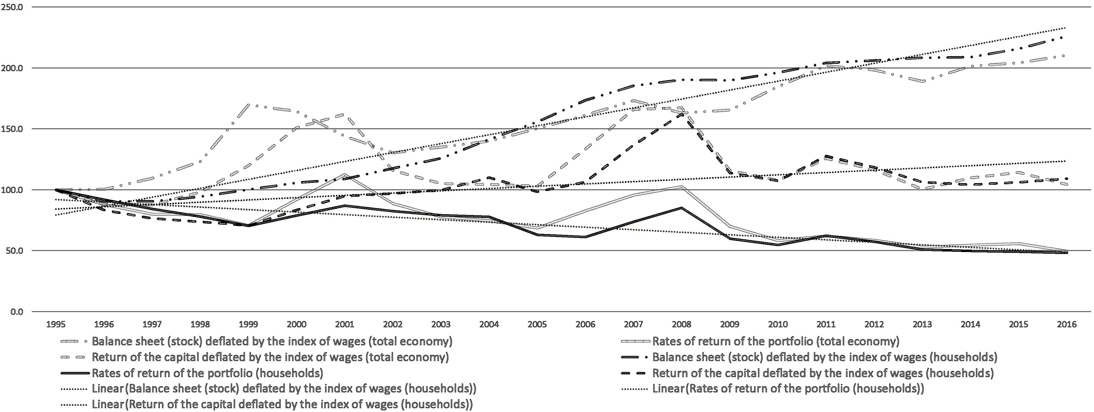
Table 5 shows how the transactions of household sector are linked with the corresponding income distribution statistics income flows. This corresponds in Table 1 to steps D and E. The grey areas in the table emphasise the differences between national accounts and income distribution statistics. As can be seen in Table 2, the share of non-comparable transactions varies between 17 and 22 percent of the primary income. However, this does not mean that the income distribution statistics do not include any corresponding transactions with the national accounts. For instance, employers’ social contributions are broken down by income deciles of wages and salaries, as these two are clearly connected. The last column in Table 2 shows the share of the non-comparable items of national income. These types of transactions represent roughly two percent of the national income. These transactions are: paid interest, reinvested earnings on direct foreign investment, investment income from collective mutual funds belonging to shareholders, investment income based on pension entitlements and investment income attributable to policyholders in insurance. In theory, investment income based on pension entitlements and investment income attributable to policyholders in insurance could be broken down into the income deciles by using the corresponding stock in the wealth survey but this is not done as the time series of the wealth survey are too short and these data are not annually available. As these transactions are also small, the error caused is minor.1212
3.Results
Figure 1 shows that the households’ balance sheets as well as the total economy balance sheets have grown particularly quickly in the past twenty years.1313 Both the balance sheets of households and total economy have doubled from 1995 to 2016 in relation to wages and salaries. In this analysis, financial stock and actual rate of returns have been “corrected” with the index of wages and salaries earnings. The reason is that this illustrates the development in relation to “a normal household” or “a working household”, i.e. how much quicker these have been developed than labour income. Without this correction, the growth would have been roughly double that shown in the graph.1414 This correction does not have any impact on the change of rate of returns, which corresponds with Piketty’s r (return on capital) as well as the other estimations/results presented later in this article.1515 It is interesting to notice that the household sector financial wealth grew more quickly than the financial wealth of the other sectors.
During the same time frame the household and total economy rates of return1616 have roughly halved. During the years of strong economic growth, like around year 2000 and before the subprime crisis (2008) the rates of returns increased but, as can be seen in the graph, the trend of returns is clearly declining. This development is logical, as at the beginning of the euro area the overall interest rates converged due to the single monetary policy and thus, in several countries – including Finland – declined compared to the past when the monetary union countries still had their own independent monetary policy. This process began at the end of 1996 when the Finnish markka was brought into the Exchange Rate Mechanism (ERM) of the European Monetary System (EMS) in which fluctuation within a band of 15 percent was allowed. At the beginning of 1999, the fixed conversion rate between the Finnish markka and euro was confirmed. After the financial crisis, interest rates crashed as the European Central Bank dropped its interest rates benchmarks to zero and overnight deposit facility rates even to negative.
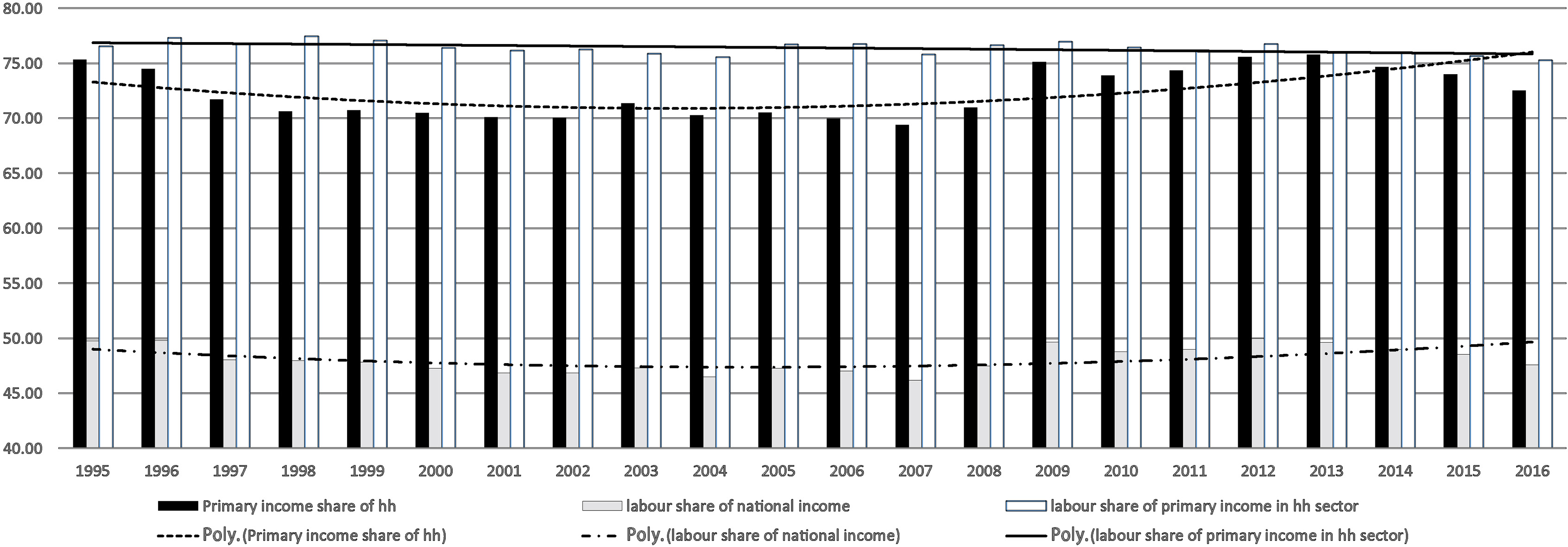
Figure 2.
Primary income share of households, labour share (compensation of employees) of national income and the labour share of primary income. Source: Statistics Finland and author’s calculations.
However, it is important to note that the underlying reason for the decreasing rates of return was not only decreasing interest, but also because the returns on shares crashed. Returns on shares are typically more volatile than interest rates and they follow the overall economic development more closely than the interest instruments. However, the trend of returns, i.e. distributed income of corporations decreased during this period. At the beginning of the 1990s the Finnish economy was in a severe depression and the profitability of corporations was overall poor. Consequently, returns were also low. The depression was followed by rapid economic growth and thus, the profits of corporations increased rapidly. The dividends and rates of return increased and this is reflected in Fig. 1 as an increase of rates of return. At the beginning of the 21
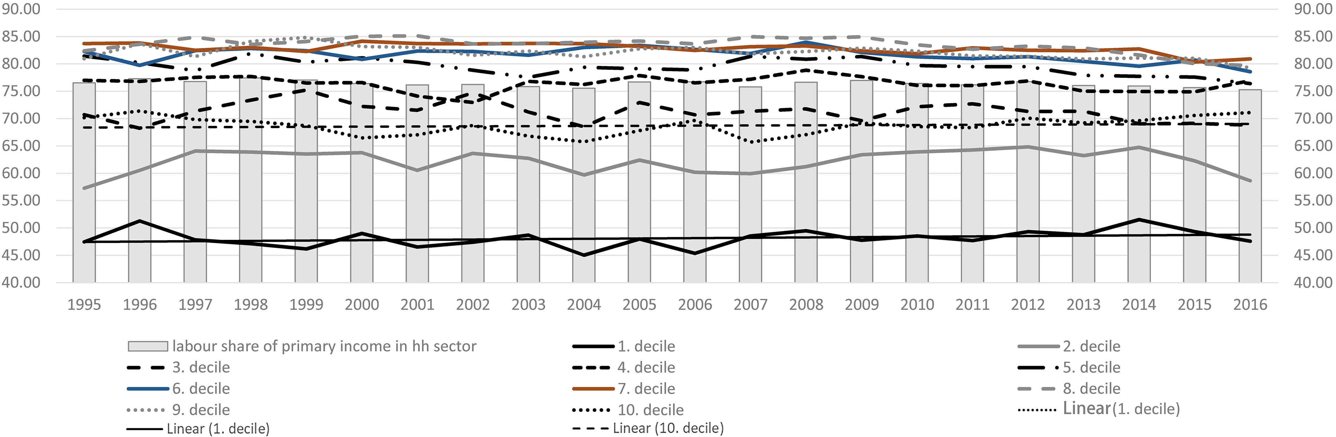
Figure 3.
Compensation of employees’ shares of primary income by income deciles and the labour share of primary income in household sector. Source: Statistics Finland and author’s calculations
Due to the decrease in the returns on dividends, the entire portfolio’s rates of returns have increased moderately. Households’ portfolio grew nine percent more quickly than wages and salaries from 1995. The entire domestic economy’s portfolio increased only 4.5 percent more quickly than wages and salaries. The rates of returns of other than interest-bearing instruments were low in 1995. Typically, the rates of returns are volatile and consequently, the actual property income is also very volatile. In 2008 the rates of return and the actual property income were above their trend but after this they fell below.
Figure 2 shows the household share of the primary income (national income), the compensation of employees as a share of national income, the compensation of employees as a share of household sector primary income (national income) for the household sector as well as broken down by income quintiles. It is important to note that the income deciles are calculated from disposable income and not from primary income even though the lines in the graph represent the compensation of employees’ shares of primary incomes broken down by income deciles. The reason is that disposable income shows the actual situation of households concerning their income and welfare and primary income does not take into account the effect of income redistribution.
In Fig. 2 the household shares of primary income are presented as a histogram with black background. During economic downturns, the share is typically larger than during periods of economic growth. The reason is that households typically mainly receive compensation of employees while the other economic sectors receive only property income. Typically, property income is considerably more volatile and decreases during economic downturns. In 1995 the share of compensation of employees was 75 percent of national income. Due to the economic depression, this was quite high. Then the share started to decrease, falling to 70 percent in 2007. After this, it continuously increased again, exceeding 75 percent in 2012/13 before beginning to decrease again.
The primary income sources belonging to households are compensation of employees and property income, as primary income belonging to other sectors is purely property income. Therefore, Piketty’s assumption that the functional income distribution of the entire economy would be reflected directly in the income distribution between households is wrong. As other sectors than households receive property income and not compensation of employees, the increasing income of these sectors increases the property income share of functional income distribution. Thus, this type of increase of property income share of functional income distribution does not have any impact on the income distribution between households.
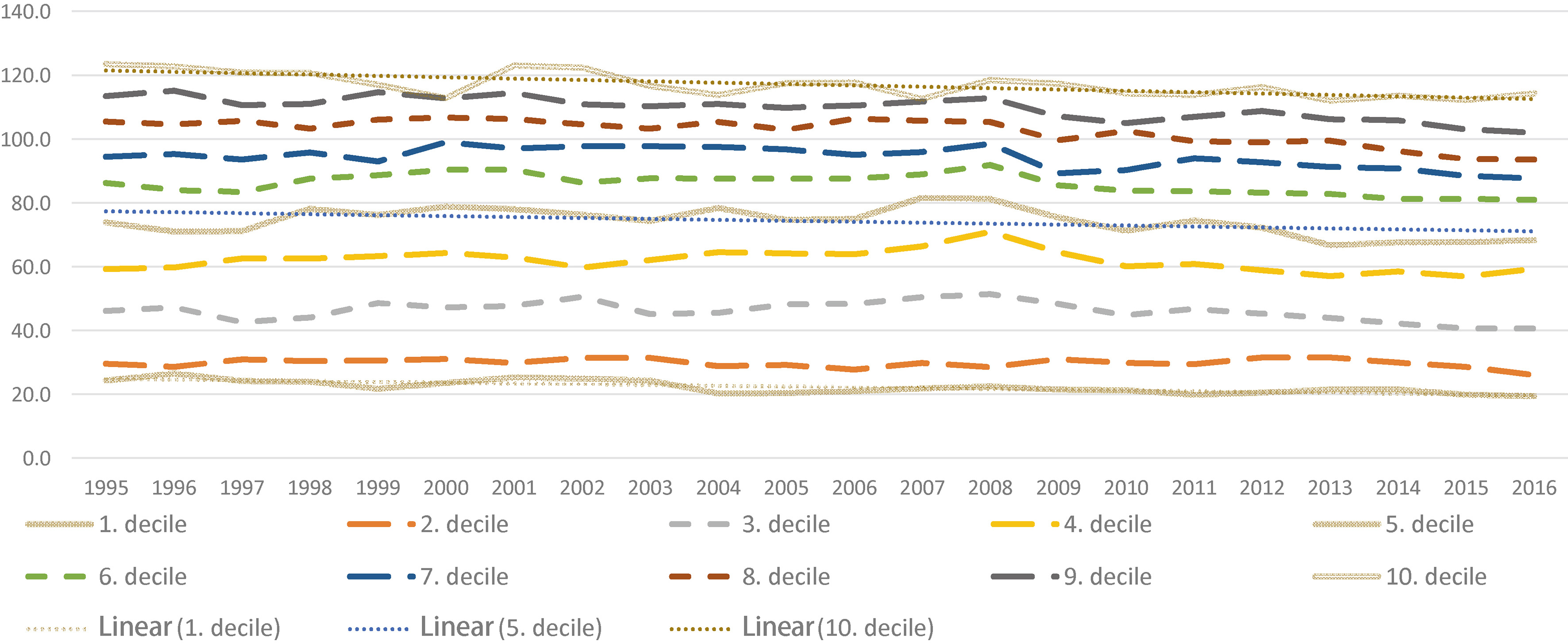
Figure 4.
The primary income share of disposable income by income decile, 1995–2016. Source: Statistics Finland and author’s calculations.
The primary income received by the other sectors is property income that they receive from their ownership. In the case of corporations, these improve their net financing position, allowing them to either pay higher dividends or invest. In the case of the third or public sector, the money is used to finance the activities of the sector.
It is important to note that when the property income share is high (inverse of the grey bar), households’ primary income share is also low (black histograms in the graph). Thus, the changes in the income shares do not transfer fully to the income distribution between households. The relation depends on the amount of financial assets held by other sectors than households. If the assets held by the other sectors are small, then the link between functional income distribution and income distribution between households is direct. In Finland, the government sector for instance has considerably greater assets. The incomes generated by these assets are used to finance the government sector.
In Fig. 2 the white histogram shows the households’ labour income share of the primary income. The share has been around 76–77 percent and the variation has been relatively small. In 2015 and 2016, the shares have been slightly below 76 percent. The lines in Fig. 3 show the compensation of employees’ shares of primary income by income deciles. The shares vary from year to year but the variation is relatively small.
In Fig. 3 the trend lines of the first (lowest) and tenth (highest) income deciles are indicated with trend lines (the actual line: black “point” dashed line next to the trend line in the middle of the graph). The lower darker trend line is the trend line of the first decile and the upper one (in the middle of the graph) the trend line of the tenth decile. As can be seen in Fig. 3 the primary income of the first income decile is overall quite low because the primary income is typically generated from assets or wages and salaries.
Figure 4 shows the primary income share of disposable income. This is an indication of the wages’, salaries’ and property income’s relation to the transfers received. The first income decile typically receives its income from transfers and thus, received wages and salaries are relatively low. The highest income deciles typically receive much property income and thus, the share of property income in the top decile is normally the highest. It is interesting to note that the primary income share of disposable income has decreased in the past years in all deciles. In practice, this means that net transfers have increased practically in all the income deciles. The underlying reason for this is demographic, i.e. as the average age increases, the households are increasingly earning pensions (transfers) instead of labour income. Partially, the impact may be explained by the relatively decreasing income and wealth taxes and increasing or less decreasing social benefits.
The labour shares of primary income in different income deciles have remained almost stable (Fig. 3). The variation of the shares in different income deciles is roughly a few percent. Typically, high-income decile families are more sensitive to changes in property income but there is clearly no structural changes in the Finnish data. The labour income shares are the highest in the seventh (grey line on the top of the graph), eighth (grey dashed line on the top of the graph), and ninth (grey “point” dashed line on the top of the graph) deciles. It is important to note that imputed rents are property income. The imputed rental income is typically more important for middle-income than for high-income families.
4.Conclusions
This article presents a framework, which starts from the balance sheets of the economy, links those with the corresponding income flows of national income, and separates the income flows that belong to the households. Finally, these flows are linked with the income distribution data, which allows scrutiny of capital and labour income by income quintiles.
This relative short analysis focuses on the years from 1995 to 2016, indicating that Piketty’s scenario, where we would enter a new belle époque, would not be realised in Finland. Financial wealth has roughly doubled in relation to wages and salaries in past twenty years. However, this has not had any impact on property income and the labour shares of different quintiles have remained almost unchanged. The main reason for this is that rates of return have collapsed.
If the rates of return remained at the same level as in the 1990s, income generation as well as distribution would have changed considerably. However, the rates of return halved, which also cancelled out the potential effect of the increase of the balance sheets. The returns varied according to the economic cycle, but the trend of returns was decreasing. At the beginning of the euro area the driving force was the decreasing interest rates, which fell overall, but the impact was particularly strong in border states like Finland. In 2008 the redistributed profits of corporations were at a record high but this was not enough to turn the overall trend of decrease. From 2008 onwards the distributed profits also fell and interest continued decreasing as well.
The approach of this article differs from Piketty’s even though it discusses the same phenomenon. As Milanovic [7] has emphasised, national income is not the same as disposable income and the link between these two is not direct. This article specifically analyses how the changes in the distribution of national income affect income distribution between households. The labour or capital – however one wants to approach it – share typically varies in time and during strong economic growth profits also increase quickly, which leads to an increasing capital share in national income. However, it is important to note that the households’ share of primary income decreases at the same time as well. The other sectors than households receive only property income and, when property income grows more quickly than labour income, the household share of primary income decreases. In Finland, the public sector holds a considerable amount of assets. If we think this as a purely statistical process, the primary income share of other sectors than households functions as a filter between the household and total economy functional income distribution. This means that the functional income distribution overestimates the property income received by households. In the Finnish case specifically, pensions1818 are partly funded and the property income generated by these pension stocks also benefit households even though they increase the capital share in the functional income distribution.
Piketty’s analysis is based on a strongly simplified world. The assumption is that increasing capital leads inescapably to increasing property income, which increases the inequality of income distribution. Piketty [14] also admits these simplifications in an article published in the book After Piketty. In his analysis, it does not really matter who owns the capital and thus, it does not take into account the importance of other economic sectors. It also does not take into account the importance of redistribution in income generation. Piketty’s analysis is supported by another French economist, Zucman [12], who analyses how rich households hide their property in tax havens.
The fact that these approaches are not necessarily completely correct does not change the possibility that increasing wealth will have an impact on income generation at some point. For instance, in societies where the public sector does not own assets or the role of the public sector in welfare policies is limited, functional income distribution is directly reflected in the income distribution between households. This means that in such societies Piketty’s model also works better than in countries like Finland. Therefore, it is essential to discuss different impacts on different societies and how different societal models affect income distribution. It should also be noted that this analysis covers only the past twenty years and it is not possible to extend it to cover centuries as Piketty did in his analysis. The data used is available in such detail only for a limited number of countries and over a limited time span. From this point of view, the compromises made by Piketty are understandable.
This article analysed how functional distributions in different income deciles have developed. Typically, in income deciles, which have relatively more property income, the capital/labour income share changes according to economic cycles. It is also important to note that the property income for several middle-income families is actually imputed rents, i.e. income flows which are imputed to them because they own the property in which they live. In the last few years the share of labour income has decreased in almost all the income deciles.
In the future it would be interesting to extend this approach to some other countries – particularly, to countries in which the public sector does not play a strong role. There is no reason to think that the prices and the rates of return would not develop in a similar manner. The money and capital markets are liberalised, and particularly within the European Union, the differences in portfolio returns should mainly be affected by the portfolio structure and to a certain extent the differences in the financial situation in different corporations. The major differences are between the countries, i.e. how much different sectors own different assets and, in particular, how rich are the third and public sectors. The larger the households’ share of assets, the more direct the relation between functional income distribution and distribution between households. Additionally, the type of redistribution policy run by the government greatly defines the final distribution of income between households. This aspect has not been covered here.
Data availability makes it difficult to replicate this exercise in other countries. The financial balance sheets, related flows, national income (including its components) and household sector (covering its flows) are relatively easily available in the European countries. It is difficult to find data that separate entrepreneurial income from the rest of the property income flows and, in particular, sufficiently detailed income distribution data. Additionally, most income distribution studies are actually surveys and not based on the register data, and therefore the coverage ratios are considerably lower than in Finland. This means that if this analysis is applied to other countries, certain compromises concerning the quality of the results most likely need to be accepted.
Notes
1 This refers to the era before WWI. This concept came into existence after WWI and refers in a romantic manner to the politically optimistic, peaceful and wealthy era. The era starts from the end of the Franco-Prussian War (1870–71) and ends with WWI.
2 van de Ven [3] has emphasised that the increasing interest in wealth depended on three factors: (1) increase of wealth – in particular increase of financial wealth; (2) in the societies as well as in political debate, an overall increase of interest in income and wealth distribution; and (3) the U.S. subprime crisis, which was trigged by the subprime loans that were granted to the low income households.
3 For instance for the U.S. these accounts are reported in [6].
5 The pure “income” concept according to national accounts without the inclusion of unrealised holding gains and losses is possible solution, but results have to monitored against this drawback, especially when comparing income on bonds and deposits vis-á-vis vis shares and mutual fund shares.
6 When comparing data, it should be mentioned that in the financial accounts business wealth is part of financial wealth, while in distributional accounts for financial wealth (HFCS) main parts of the business wealth is attributed to non-financial wealth other than dwellings and land. To illustrate the importance: Half of the property income of households in the EU-19, 65% in Finland is attributed to distributed income on corporations.
7 The rates of returns are based on the assumption that these measures are consistent. The stocks and the related income flows are calculated separately, and thus an error/inconsistency might appear in the rates of returns. This would appear as overly low or high rates of returns as well as discrepancies between net lending/borrowing calculated based on financial and non-financial accounts.
8 In theory, the household population between the national accounts and income distribution statistics should be the same, except concerning the coverage of institutionalised households. These are covered in the national accounts and excluded from the income distribution statistics. Institutionalised households refer to households which are in institutions like hospitals and prisons for a long period of time or permanently. More on the coverage of income distribution statistics and national accounts: [11].
9 This corresponds in the bookkeeping with the concept of EBIT (earnings before interest and taxes).
10 This corresponds in the bookkeeping with the concept of EBT (earnings before taxes).
11 In practice this is operating surplus generated by owner-occupied housing and from which corresponding (mortgage) interest flows are deducted.
12 This might vary from country to country, e.g. taking into account examples like the Netherlands with high proportion of pension capital and consequently high proportion of related income.
13 A main reason of the increase is the revaluation of financial wealth.
14 Wages and salaries grew by 93 percent from 1995 to 2016.
15 It is important to notice that the rates of returns do not cover realised or non-realised holding gains. In the national income estimations these are classified as price changes rather than income. This same assumption applies to Piketty’s calculations.
16 Defined as property income (as defined in the national accounts) divided by the underlying stock of financial assets.
17 The assumption in calculating the rates of returns is that financial and non-financial accounts are consistent. The indication of consistency is that the net lending/borrowing based on non-financial accounts is consistent with the net lending/borrowing based on the financial accounts. In the Finnish national accounts this is not the case and thus, this discrepancy may cause a relatively small error in the calculations.
18 Classified as social security pensions in national accounts.
Acknowledgments
I would like to thank Frank Trentmann (Birkbeck Colleague and University of Helsinki) and Michael Andreasch (Oesterreichische Nationalbank) for their valuable comments.
References
[1] | Piketty T. Capital in the Twenty-First Century, The Belknap Press of Harvard University Press, (2014) . |
[2] | Stiglitz J, Sen A, Fitoussi J-P. Report by the Commission on the Measurement of Economic Performance and Social Progress, (2009) , www.stiglitz-sen-fitoussi.fr (referred 15.8.2019). |
[3] | Van de Ven P. Present and future challenges to the system of national accounts: Linking micro and macro, Review of Income and Wealth. (2017) ; 63: : S266-S286. |
[4] | IMF ja FSB, The Financial Crisis and Information Gaps, Report to the G-20 Finance Ministers and Central Bank Governors, 2009, http://www.financialstabilityboard.org/ publications/r_091107e.pdf (referred 15.8.2019). |
[5] | Kavonius IK, Honkkila J. Developing Distributional Household Balance Sheets, 9, Irving Fisher Committee Bulletin No 49: Are post-crisis statistical initiatives completed? Bank for International Settlements, Vol. 2019/49, https://www.bis.org/ifc/publ/ifcb49.pdf (referred 15.8.2019). |
[6] | Piketty T, Saez E, Zucman G. Distributional national accounts: methods and estimates for the United States, The Quarterly Journal of Economics. (2016) ; 133: : 553-609. |
[7] | Milanovic B. Increasing Capital Income Share and its Effect on Personal Income Inequality, Boushey H, Delong J B and Steinbaum M. (ed.), After Piketty – The Agenda for Economies and Inequality, Harvard University Press, (2017) . |
[8] | Krugman P, Why We’re in New Gilded Age, Boushey H, Delong J B and Steinbaum M. (ed.), After Piketty – The Agenda for Economies and Inequality, Harvard University Press, (2017) . |
[9] | Solow R. Thomas Piketty is Right, Boushey H, Delong J B and Steinbaum M. (ed.), After Piketty – The Agenda for Economies and Inequality, Harvard University Press, (2017) . |
[10] | Kavonius IK. Varallisuus tuloerojen taustalla: Analyysi varallisuuden ja tulonjaon välisestä yhteydestä vuosina 1995–2016, Kansantaloudellinen Aikakauskirja. (2019) ; 115: : 24-40. |
[11] | Kavonius IK, Törmälehto V-M. Household income aggregates in micro and macro statistics, Statistical Journal of the United Nations Economic Commission for Europe. (2003) ; 23: : 9-25. |
[12] | Zucman G. The missing wealth of nations: are Europe and the U.S. net debtors or net creditors? Quarterly Journal of Economics. (2013) ; 128: : 1321-1364. |
[13] | Törmälehto V-M. Tulo-, kulutus ja varallisuuseroista Suomessa, Kansantaloudellinen Aikakauskirja. (2019) ; 115: : 41-65. |
[14] | Piketty T. Toward a Reconciliation between Economics and the Social Sciences, Boushey H, Delong J B and Steinbaum M. (ed.), After Piketty – The Agenda for Economies and Inequality, Harvard University Press, (2017) . |


