An estimating parameter of nonparametric regression model based on smoothing techniques

1.Introduction

In statistical modelling, regression analysis is a statistical process for estimating parameters of the relationships between dependent and independent variables in terms of a regression function. However, regression analysis requires an assumption of the underlying regression function to be met. If an inappropriate assumption is used, it is possible to produce misleading results. To overcome this problem, the nonparametric regression is a choice to analyze data when the data are not meeting the assumption of regression analysis. The nonparametric regression is an alternative way for looking at scatter diagram smoothing to depict the relationship between dependent and independent variables. The single independent variable is called scatterplot smoothing it can be used to enhance the visual appearance to help our eyes pick out the trend in the plot.

The smoothing technique is a part of a method to estimate unknown parameters (trend or smoothing estimators) of nonparametric regression models. There are many popular smoothing techniques such as the smoothing spline [1, 2], the penalized spline [3], and the B-spline [4]. The estimating parameters of these methods depend on the smoothing parameter which is controlled the trade-off between fidelity to the data and roughness of function. Smoothing Spline (SS) is a technique that estimates the natural polynomial spline by minimizing the penalized sum of squares based on a smoothing parameter. The penalized Spline (PS) smoother is approximated by minimizing the truncated power function on a low rank thin-plate spline depended on the smoothing parameter. The concept of the B-spline is similar to the smoothing spline and penalized spline. This requires the piecewise constant B-spline that can be obtained from truncated counterparts by differencing the B-spline function.

In this paper, we consider the nonparametric regression model in Section 2, and use the smoothing spline, penalized spline, and B-spline methods to estimate the unknown parameter of nonparametric regression model in Section 3. In Sections 4 and 5, we show the estimation of these methods for simulation data and real data. The conclusion is presented in Section 6.

2.The nonparametric regression model

The nonparametric regression model consists of the cubic spline of piecewise polynomials function based on a function of independent variables (S⁢(xt)), error process (εt), and dependent variables (yt) following

The error process is assumed to follow the normal distribution with mean zero and variance one.

3.Method of smoothing techniques

The following smoothing techniques show the process to estimate parameters based on nonparametric regression model.

3.3B-spline method

B-splines are very interesting as a basic function for univariate independent variable of nonparametric regression function. De Boor [10] gave an algorithm to compute B-spline of lower degree on piece wise polynomials function.

The mth degree of B-spline function are evaluated from (m-1)th degree as

(15)

Bjm⁢(x)=xt-τjτj+m-1-τj⁢Bjm-1+τj+m-xtτj+m-τj+1⁢Bj+1m-1,

where basis of order m with knots {Bim|i=M-m+1,…,M+K}, and auxiliary knots τj. B-splines base on non-zero over domain spanned by at most M+1 knots. In this case, we focus the m= 4 or called the cubic B-spline with K knots has basis expansion as

S⁢(xt)=∑j=1K+4Bj4⁢(xt)⁢βj.

The nonparametric regression model can written in form of B-splines as

(16)

yt=∑j=1K+4Bj4⁢(xt)⁢βj+εt,t=1,2,3,…,n.

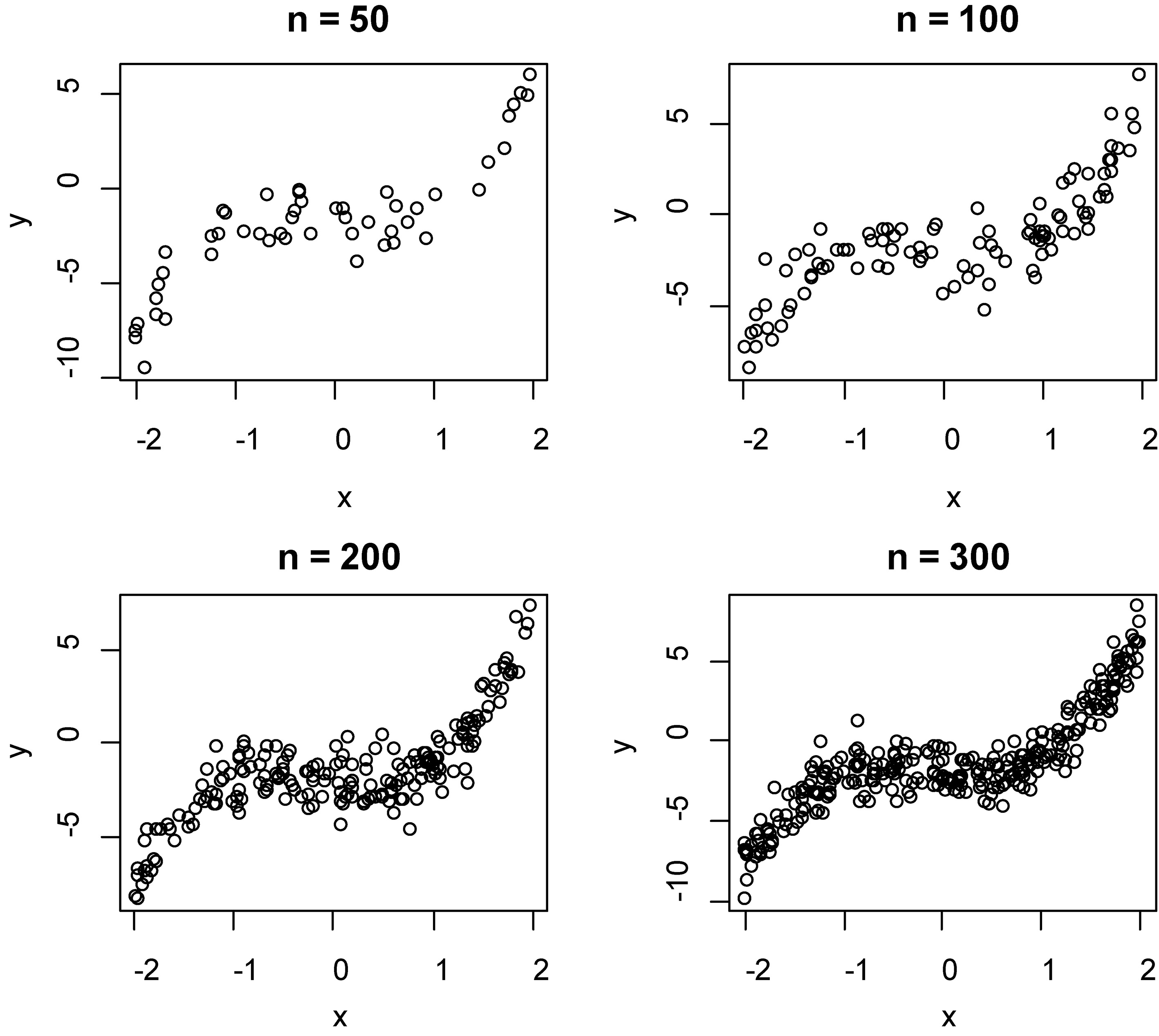
Figure 1.

The scatter plot of dependent and independent variables on model 1.

In matrix form, B-splines can be written in form a linear model

B=[B14⁢(x1)…BK+44⁢(x1)⋮⋮B14⁢(xn)…BK+44⁢(xn)],⁢y=[y1y2⋮yn],

 and ⁢ε=[ε1ε2⋮εn].

The B-splines estimators are approximated by least square problems as

⁢β^=[β^1β^2⋮β^K+4]=(BT⁢B)-1⁢BT⁢⁢y.

The B-spline and penalties are studied by Eilers and Marx [4] that advocate the use of the equally spaced knots, instead of the order statistics of the independent variable. The B-spline coefficients can be estimated as

(17)

⁢β^=(BT⁢B+λ⁢DT⁢D)-1⁢BT⁢⁢y,

where D is a banded matric which correspond to the difference penalty and denote by

D=[000⁢…⁢00-110⁢…⁢000-11⁢…⁢00…………000⁢…-11].

The fitting cubic B-splines are S^⁢(xt)=∑j=1K+4Bj4⁢(xt)⁢β^j. The smoothing parameter λ choosing by minimizing the ordinary function or the generalized cross-validation function.

Figure 2.

The scatter plot of dependent and independent variables on model 2.

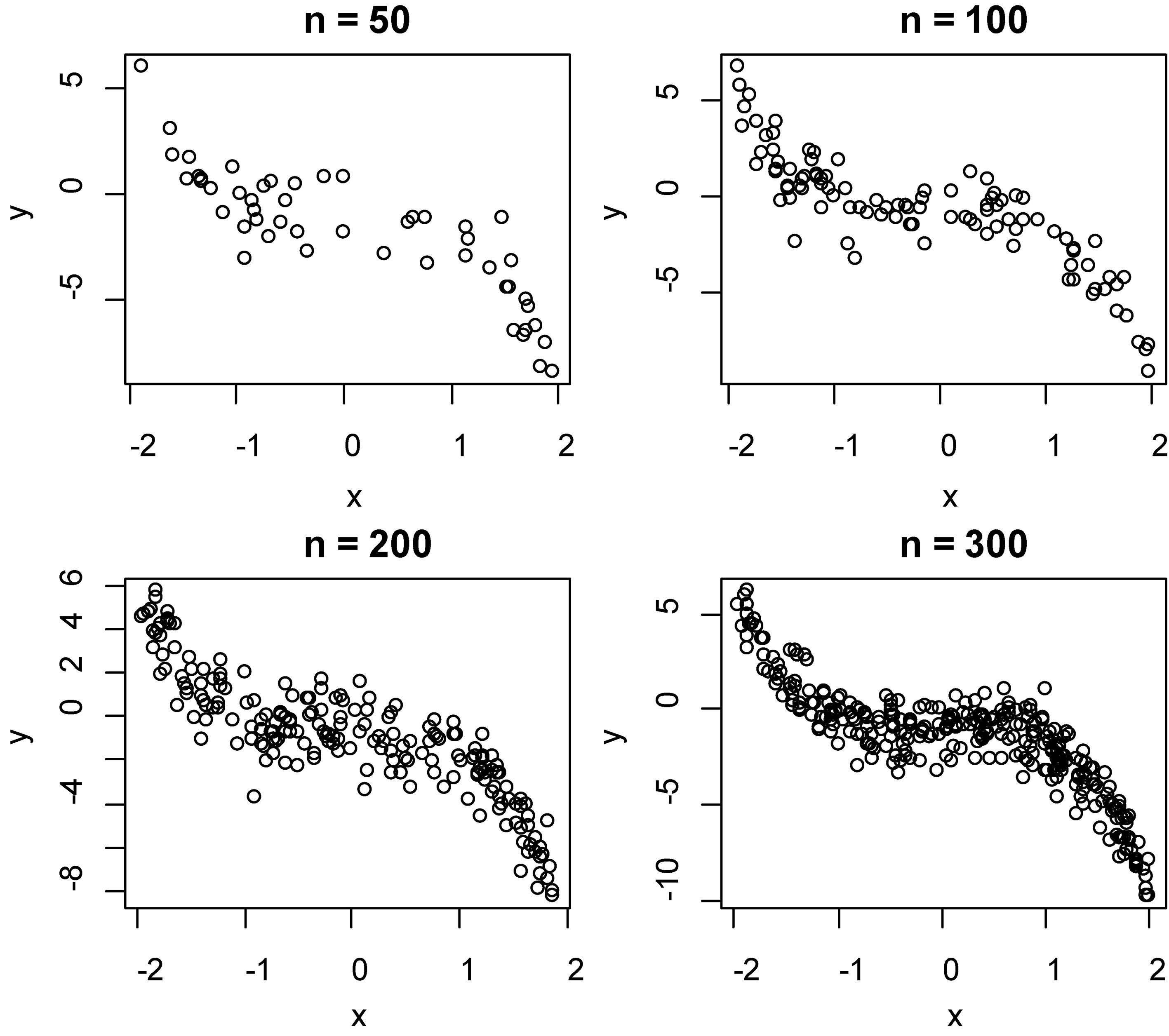
Table 1

The summary statistics of simulation studies with model 1 based on smoothing spline (SS), penalized spline (PS), and B-spline (BS)

Sample sizes	Methods	Mean		S.D.		LCI		UCI		t-statistic		p-values
n= 50	SS	-0.	3344	6.	5444	-0.	9095	0.	2405	-1.	1428	0.	2537
	PS	-0.	3484	6.	7454	-0.	9411	0.	2442	-1.	1552	0.	2468
	BS	0.	3666	6.	6935	-0.	2214	0.	9548	1.	2249	0.	2212
n= 100	SS	0.	0719	4.	2680	-0.	3031	0.	4469	0.	3767	0.	7065
	PS	0.	0837	4.	2029	-0.	2855	0.	4530	0.	4454	0.	6562
	BS	-0.	0895	4.	2152	-0.	4599	0.	2807	-0.	4751	0.	6349
n= 200	SS	-0.	0954	2.	8932	-0.	3504	0.	1595	-0.	7353	0.	4625
	PS	-0.	0921	2.	9123	-0.	3480	0.	1637	-0.	7072	0.	4798
	BS	0.	0149	3.	2685	-0.	2299	0.	2598	0.	1200	0.	9045
n= 300	SS	-0.	1574	4.	2673	-0.	5347	0.	2197	-0.	8201	0.	4125
	PS	-0.	1441	4.	1982	-0.	5130	0.	2247	-0.	7676	0.	4431
	BS	0.	1475	1.	8514	-0.	2786	0.	5738	0.	6802	0.	4966

Table 2

The summary statistics of simulation studies with model 2 based on smoothing spline (SS), penalized spline (PS), and B-spline (BS)

Sample sizes	Methods	Mean		S.D.		LCI		UCI		t-statistic		p-values
n= 50	SS	-0.	0037	24.	2710	-2.	1363	2.	1288	-0.	0034	0.	9972
	PS	-0.	2582	23.	8736	-2.	3559	1.	9893	-0.	2419	0.	8089
	BS	-0.	3230	27.	1906	-2.	7121	2.	0660	-0.	2656	0.	7906
n= 100	SS	-0.	3966	15.	8261	-1.	7871	0.	9939	-0.	5603	0.	5755
	PS	-0.	2489	16.	4557	-1.	6947	1.	1969	-0.	3382	0.	7353
	BS	0.	5461	16.	2381	-0.	8806	1.	9729	0.	7520	0.	4524
n= 200	SS	-0.	3704	8.	1031	-1.	0838	0.	3430	-1.	0201	0.	3082
	PS	-0.	3447	7.	8716	-1.	0363	0.	3468	-0.	9792	0.	3279
	BS	0.	4035	8.	5116	-0.	3443	1.	1514	1.	0602	0.	2896
n= 300	SS	0.	0411	7.	3081	-0.	6055	0.	6878	0.	1250	0.	9005
	PS	0.	0408	7.	0664	-0.	5800	0.	6617	0.	1291	0.	8973
	BS	0.	0344	7.	2205	-0.	5999	0.	6688	0.	1066	0.	9151

4.Simulation study

The nonlinear data of this study is simulated in two models for estimating the performance of smoothing techniques based on independent variables which are considered in the class of uniform distribution. These models in the process of construction a curve on mathematical function, that show the best fit to a series of data points. Figures 1 and 2 show the scatter plot of xt and yt on models 1 and 2 with 50, 100, 200, 300 sample sizes.

Model 1

Model 2

The next step, the estimates of S⁢(xt) or called S^⁢(xt) are approximated from smoothing spline (SS), penalized spline (PS), and B-spline (BS) that used to compute the bias and MSE of S⁢(xt) following

The data are generated and repeated for fitting the model 500 times. A t-statistic is adopted to test that the mean of bias is equal the zero or called unbiased estimator. Tables 1 and 2 present the various summary statistics for the smoothing estimator obtained from three methods. The third and the fourth columns of these tables represent the sample mean and standard deviation of biases. The sample mean for the lower and upper bounds of the 95% confidence interval are given in the next two columns. The last two columns of these tables list the t-statistic, and p-values for hypothesis testing (H0:μS𝑏𝑖𝑎𝑠=0⁢ versus ⁢H0:μS𝑏𝑖𝑎𝑠≠0) that means when reject H0:μS𝑏𝑖𝑎𝑠=0 the estimator SS, PS, and BS with bias. The histogram of the bias estimator of SS, PS, and BS in model 1 are presented in Figs 3–5, and model 2 are presented in Figs 6–8.

Figure 3.

Histogram of bias for fitting data of smoothing spline method with model 1.

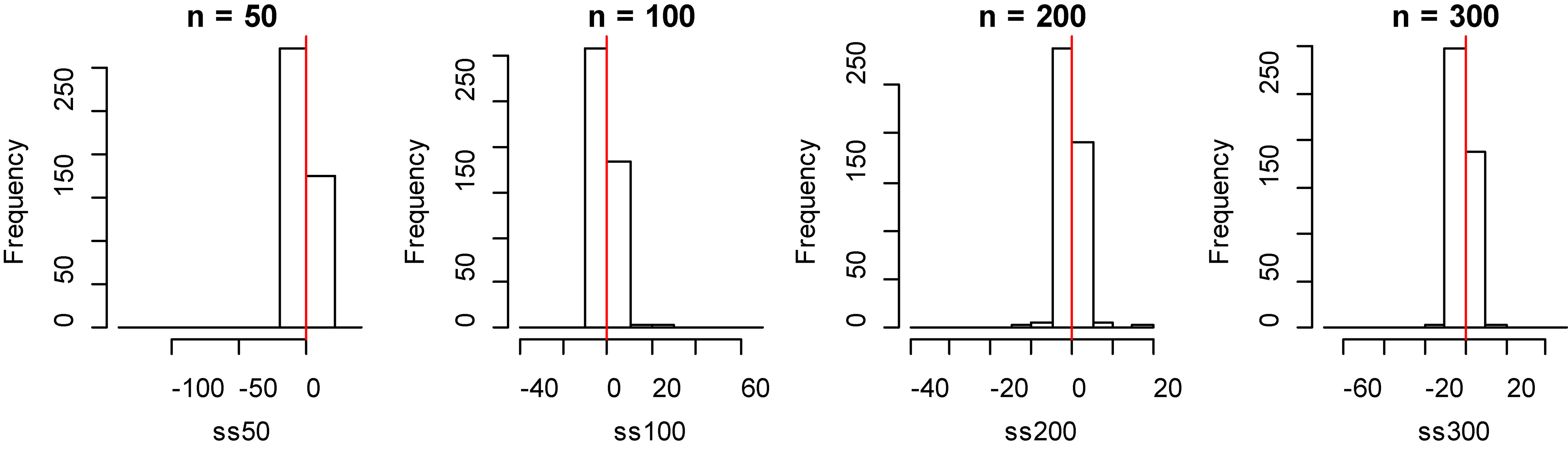
Figure 4.

Histogram of bias for fitting data of penalized spline method with model 1.

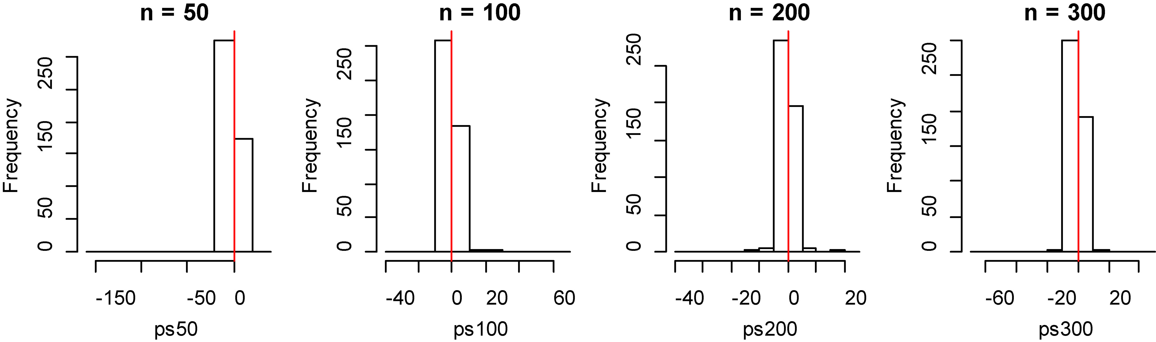
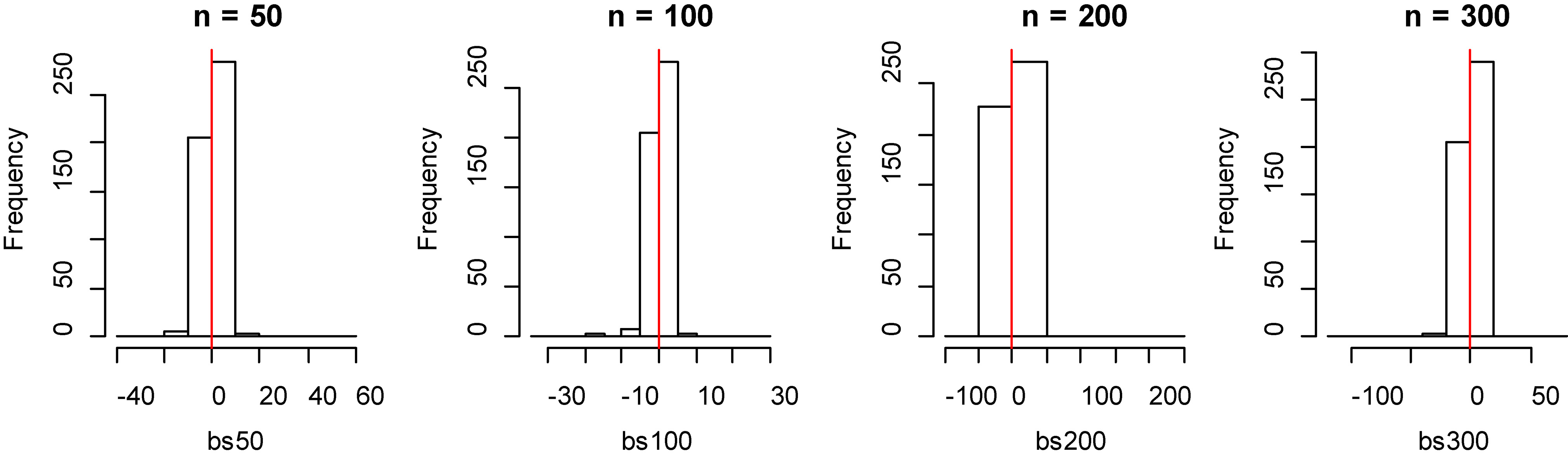
Figure 5.

Histogram of bias for fitting data of B-spline method with model 1.

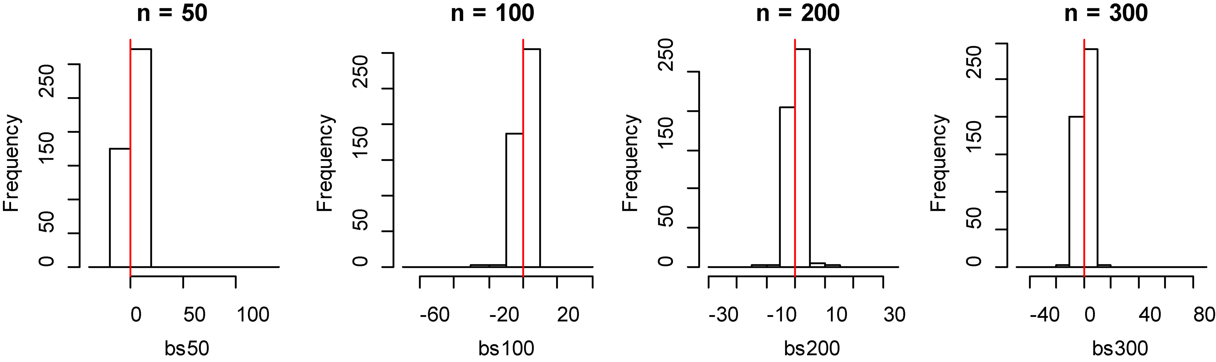
Figure 6.

Histogram of bias for fitting data of smoothing spline method with model 2.

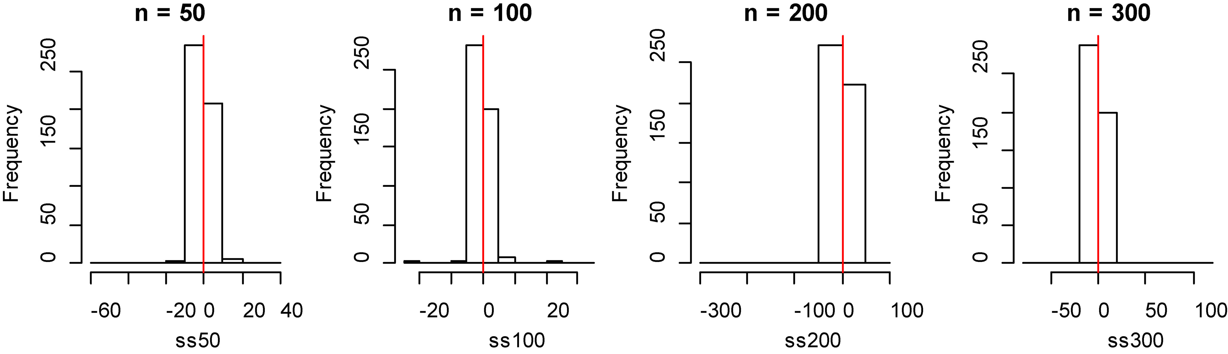
Figure 7.

Histogram of bias for fitting data of penalized spline method with model 2.

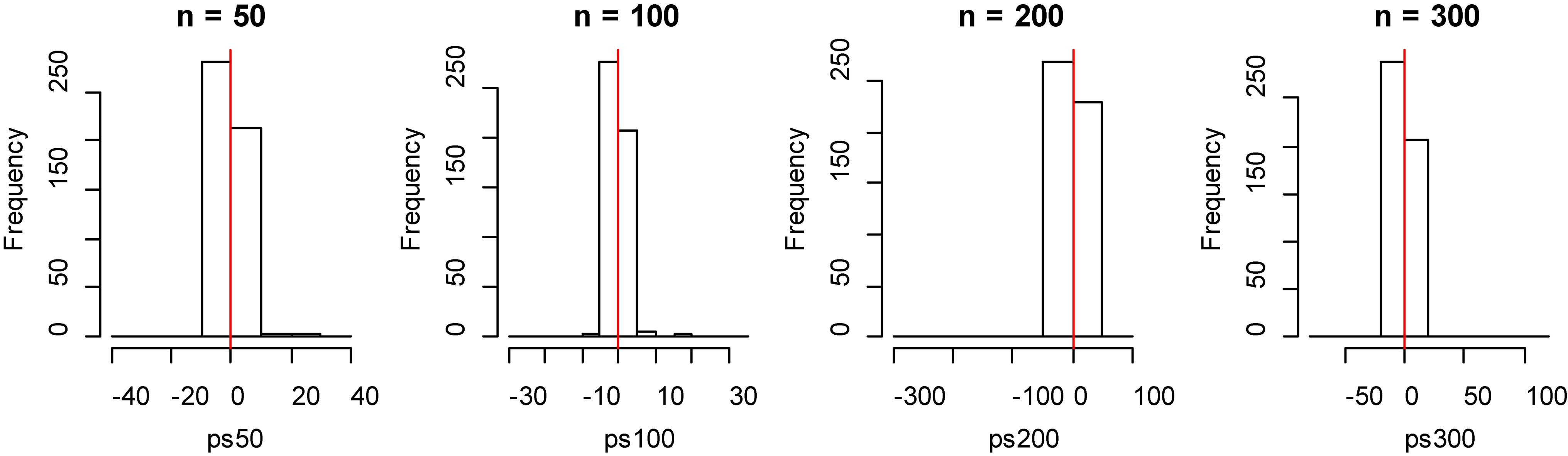
Figure 8.

Histogram of bias for fitting data of B-spline method with model 2.

From Tables 1 and 2, by observing the p-values, the SS, PS, and BS provide asymptotically unbiased estimates for estimating parameter of S⁢(xt) nearly for all sample sizes of two models. From the p-values for the two tables it is seen that are seen that the SS, PS, and BS of smoothing method have a good performance to fit data in a class of nonlinear data. From the histogram it is apparent that a standard deviation of relative biases increase with increasing sample sizes, so it makes the leptokurtic distribution. The average of MSE can answer the final question which smoothing method is the best estimator. Table 3 shows the average MSE for fitting 500 times on two models, and it can be seen that the PS method shows the minimum of average MSE for all sample sizes and models.

Figure 9.

The plot of LIDAR data frame and model fitting of SS, PS, and BS methods.

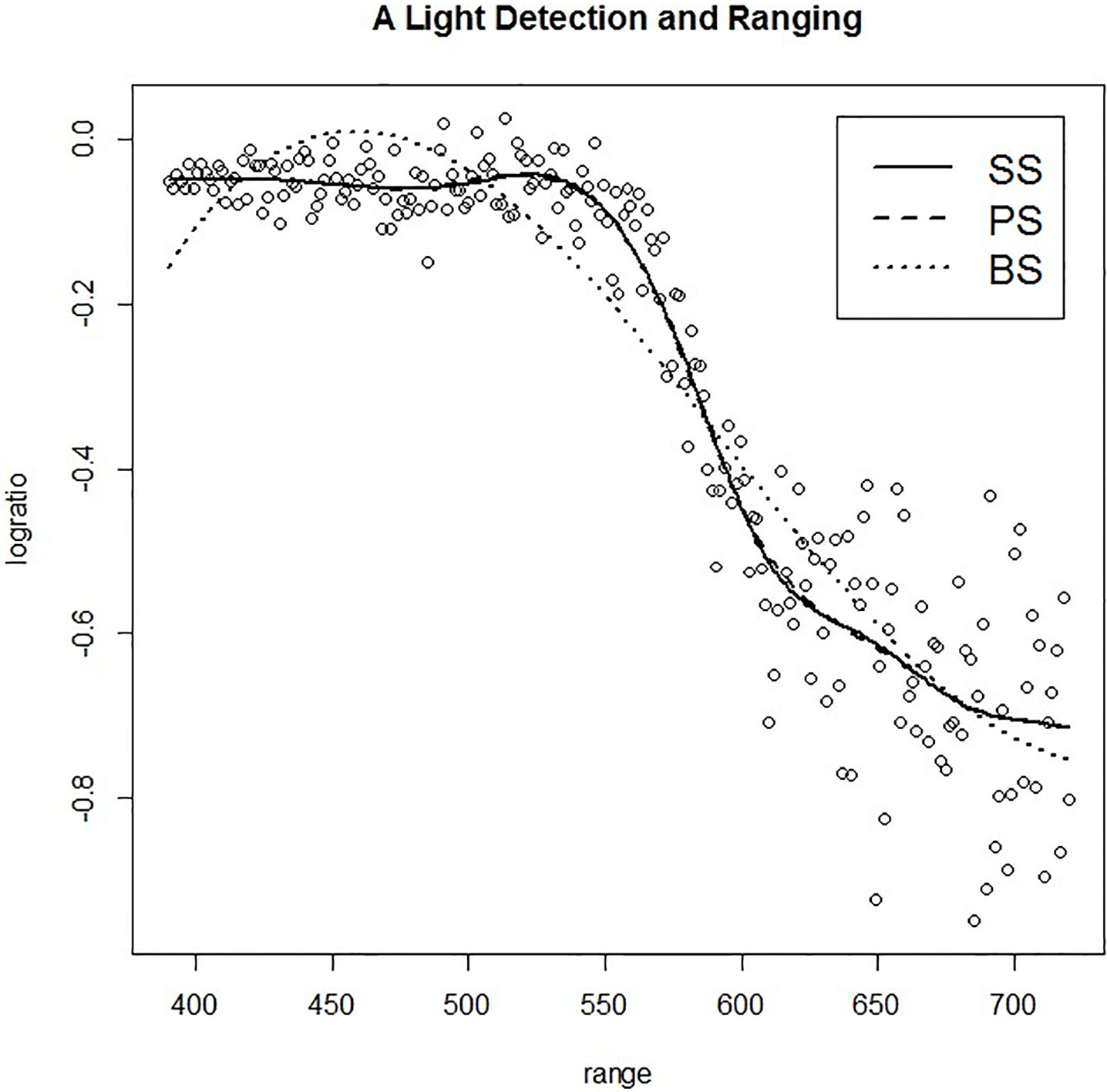
5.Application of real data

In this section, we consider the application of smoothing method based on SS, PS, and BS methods that we developed in the previous section. As the real data, we use the data frame which consists of 221 observations from a light detection and ranging (LIDAR) experiment. This data frame contains the range distance travelled before the light is reflected back to its source and logarithm of the ratio of received light from two laser sources as shown in the plot in Fig. 9.

After fitting the model, the estimating values play on a plot of light detection of ranging. It can be seen that the SS and PS interpolate in mass data more than the BS method that followed the MSE values such as SS = 0.006016, PS = 0.006010, and BS = 0.009288. The minimum of MSE is the PS which is closed the SS as the result on Table 3.

6.Conclusion

In this section, we used the smoothing techniques of SS, PS, and BS methods based on nonparametric regression models. Through a Monte Carlo simulation study, we evaluated the smoothing estimator of SS, PS, and BS methods. For hypothesis testing based on the p-value, the fitting values supported the null value, and showed that the smoothing estimators work reasonably well for all methods, but the PS shows the minimum of average MSE.

References

[1] | Wahba G. Spline Models for Observational Data, SIAM: Philadelphia; (1990) . |
[2] | Green PJ, Silverman BW. Nonparametric Regression and Generalized Linear Models: A Roughness Penalty Approach, Chapman and Hall: London; (1994) . |
[3] | Ruppert D, Wand MP, Carroll RJ. Semiparametric Regression, Cambridge University Press: New Your; (2003) . |
[4] | Eilers PHC, Marx BD. Flexible Smoothing with B-splies and Penalties, Statistical Science 11: (2) ((1996) ), 89–102. |
[5] | Wahba G. A survey of some smoothing problems and the method of generalized cross-validation for solving them, In Proceeding of the Conference on the Application of Statistic, (1976) , pp. 507–523. |
[6] | Craven P, Wahba G. Smoothing noisy data with spline functions: estimating the correct degree of smoothing by the method of generalized cross-validation, Numerische Mathematik 31: ((1979) ), 377–403. |
[7] | Eubank RL. Spline Smoothing and Nonparametric Regression, Marcel Dekker: New York; (1988) . |
[8] | Eubank RL. Nonparametric Regression and Spline Smoothing, Marcel Dekker: New York; (1999) . |
[9] | Ruppert D, Carroll RJ. Spatial-adaptive penalties for spline fitting Australian and New Zealand Journal of Statistics 42: ((2000) ), 205–224. |
[10] | De Boor C. A Practical Guide to Splines, Springer: Berlin; (1978) . |