Quality measures for multisource statistics

3.1Mean squared error of level estimates affected by classification errors – BDC 1 “multiple non-overlapping cross-sectional microdata sets”

In this example we assume that we have several non-overlapping data sets together covering the entire target population and that the only source of errors are classification errors. In this section we will assume that the data are on businesses, which are classified by industry code (main economic activity). The unobserved true industry code of unit i is denoted by si; the observed industry code that is prone to errors is denoted by s^i. The set of possible industry codes is denoted by ℋ.

Let θ=f⁢(y1,…,yN,s1,…,sN) denote a target parameter and yi stand for the value of a target variable for unit i. Based on the observed data, this parameter is estimated by θ^=f⁢(y1,…,yN,s^1,…,s^N). We are interested to estimate the mean squared error of θ^ as affected by classification errors. We assume that the values of the target variable, y1,…,yN, are error-free.

[3] assumes that a business i with a true industry code g is classified as falling into class h with probability pg⁢h⁢i due to classification error. They propose the following method for computing the mean squared error of θ^. The first step is to estimate the probabilities pg⁢h⁢i. This requires an independent collection of data on the classification variable, where observed and cleaned versions of those data are needed. Options to obtain such data are:

Together the estimated probabilities p^g⁢h⁢i form a transition matrix 𝐏^i=(p^g⁢h⁢i). The transition matrix, per unit, can be modelled as a function of background variables. See [3] for an example.

The second step is to estimate bias and variance of θ^ by drawing bootstrap samples from 𝐏^i. For each unit we draw a new value for the industry code, given the original observed industry code s^i, according to 𝐏^i. Based on the results for this draw, denoted by s^i⁢r, we compute θ^r=f⁢(y1,…,yN,s^1⁢r,…,s^N⁢r). We repeat this procedure R times, thus r=1,…,R, and use the set of outcomes θ^r to compute estimates of the bias and variance of θ^:

with mR⁢(θ^)=1R⁢∑r=1Rθ^r.

When the target parameter θ concerns a vector of stratum totals (level estimates), one can also estimate the bias and variance-covariance matrix through analytical formulae, with R→∞: (cf. [3]):

where superscript t indicates taking the transpose, ‘*’ superscript indicates the analytical expression, 𝐈 is an identity matrix, 𝒚^=∑i=1N𝒂^i⁢yi stands for a vector of estimated stratum totals and 𝒂^i=(a^1⁢i,…,a^|ℋ|⁢i)t is a vector of dummy variables that describes in which stratum unit i is observed (a^h⁢i= 1 if s^i=h and a^h⁢i= 0 otherwise). In particular, it follows that the bias of the estimated total in stratum h, Y^h=∑i=1Na^h⁢i⁢yi, can be estimated by

and its variance can be estimated by

[4] developed a method to estimate quarterly turnover by Dutch consumers on European webshops. To that end, they use the tax file returns in the Netherlands, which includes selling of goods and services by European webshops to Dutch customers. From the tax data, quarterly turnover figures can be derived for companies that exceed a certain turnover threshold. The smaller companies are not considered. The challenge of the methodology is to identify which of the records in those tax data concern European webshops. These records are identified using a binary classifier, based on machine-learning, which separates the companies into those that belong to European webshops and those that do not. The predictions by the algorithms are not error-free, they make classification errors. In this example we explain how the uncertainty of the estimated quarterly turnover due to those classification errors is estimated.

[4] constructed a training data set of 180 companies and a test set of 79 companies by manually classifying them. Within the training data set, 76 webshops were identified and within the test set of 79 companies 13 webshops were identified.

Using the training set, the parameters of the machine-learning algorithms were estimated. These trained algorithms were used to predict the scores s^i for the units in the test set and compare them with the true scores si. For the final algorithm, the result is shown in the transition matrix below, with si given as the rows and s^i as the columns. The top row concerns having a webshop, the bottom row having no webshop.

[4] assumed that this transition matrix is the same for all units i in the population.

Next, the machine-learning model was used to predict s^i for the units not in the training set. Denote 𝒂i for the 2-vector [𝐼𝑛𝑑(si=1),𝐼𝑛𝑑(si=0)]t, where Ind stands for an indicator variable. The authors of [4] were interested in the aggregate turnover 𝒚=∑i∈C𝒂i⁢yi where C stands for the population of companies. The turnover in the first class, i.e. with 𝐼𝑛𝑑(si=1), is the target parameter. For the units in the training set, denoted by CM, the values of the vector 𝒂i are determined manually and considered to be error-free. For the remaining units 𝒂i is predicted by the machine-learning algorithm. The total aggregated turnover is estimated by

where 𝒚M stands for turnover of units in the training set which are checked manually, 𝒚A stands for the true turnover of units not in the training set but which are classified by the algorithm, 𝒚^A stands for the estimate of 𝒚A, and B^∞*⁢(𝒚^A) is the estimated bias of 𝒚^A [cf. expression (1)]. The variance of the final turnover estimate 𝒚^ is estimated in [4] by (2⁢𝐈-𝐏^t)⁢𝑉𝑎𝑟^∞*⁢(𝒚^A)⁢(2⁢𝐈-𝐏^t)t, with 𝑉𝑎𝑟^∞*⁢(𝒚^A) given by Eq. (3.1). This variance estimate ignores the additional uncertainty due to estimating 𝐏. Note that 𝒚M does not contribute to the variance.

The final results on companies estimated to be European retailers with a webshop can be found in Table 1 (taken from [4]). The manually checked turnover of European webshops, yM⁢1, consists of about half the value of the total estimated turnover, y^1. The estimated bias of y^A⁢1 varied considerably over the years with the largest values in 2014. The estimated standard deviation of y^1 suggests that the margin around the final estimate is still rather large. If we assume a normal distribution, the 95% confidence interval around y^1 in 2014 would be 837 ± 190. This corresponds to a relative margin of 22%.

[5, 6] propose an extension of the approach in this section in order to quantify the effect of classification errors on the accuracy of growth rates in business statistics, rather than the effect on the accuracy of level estimates.

3.2Variance of estimates based on reconciled microdata containing measurement errors – BDC 2 “overlapping variables and units”

The situation in this example is that a categorical target value is measured for each individual unit (with measurement error) in several data sources. We assume that a Latent Class (LC) model is used to estimate the true values of this target variable. The quality of estimates based on the reconciled microdata is then measured by the estimated variance of these estimates.

Let 𝒀=(Y1,Y2,…,Ys)t denote a vector of observed categorical variables that measure the same conceptual variable of interest (for instance, in s different data sources). The true value with respect to the variable of interest is represented by a latent class variable X. We assume for convenience that all variables Yj and X have the same set of categories, say {1,…,L}. The marginal probability Pr⁡(𝒀=𝒚) of observing a particular vector of values 𝒚=(y1,y2,…,ys)t can be expressed as the sum of the joint probabilities

over all possible latent classes:

A common assumption in LC analysis is that the classification errors in different observed variables are conditionally independent, given the true value (local independence), i.e.

In combination with Eq. (2), this leads to the basic LC model

Estimating the LC model amounts to estimating the probabilities in this expression. Probabilities of the form Pr⁡(Yj=yj|X=x) provide information about classification errors in the observed data. For example, units that in reality belong to the first category of the target variable (X=1) are misclassified on observed variable Yj with probability Pr⁡(Yj≠1|X=1)=1-Pr⁡(Yj=1|X=1). This can be seen as a quality measure for the quality of the j-th observed variable.

The model can also be used to estimate, for each unit in the data, the probability of belonging to a particular latent class, given its vector of observed values. Using Bayes’ rule, it follows that:

Edit restrictions, for instance the edit restriction that someone who receives rent benefit cannot be a home owner, can be imposed by setting certain conditional probabilities equal to zero; for instance:

The so-called MILC method (see [7]) takes measurement errors into account by combining Multiple Imputation (MI) and LC analysis. The method starts with linking all data sets on the unit level, and then proceeds with 5 steps.

[7] applied the MILC method on a combined data set to measure home ownership. This combined data set consisted of data from the LISS (Longitudinal Internet Studies for the Social sciences) panel from 2013 and a register from Statistics Netherlands from 2013. From this combined data set, they used two variables indicating whether a person is a home-owner or rents a home as indicators for the imputed “true” latent variable home-owner/renter (or other). The combined data set also contained a variable measuring whether someone receives rent benefit from the government. A person can only receive rent benefit if this person rents a house. Moreover, a variable indicating whether a person is married or not was included in the latent class model as a covariate. The three data sets used to combine the data are:

These data sets were linked on a unit level, and matching was done on person identification numbers. Not every individual is observed in every data set. This causes that some missing values are introduced when the different data sets are linked on a unit level. Full Information Maximum Likelihood (see, e.g. [9]) was used to handle the missing values when estimating the LC model. The MILC method was applied to impute the latent variable home owner/renter (or other) by using two indicator variables and two covariates.

As already explained, the MILC method can be used to assess the quality of the input sources. In Table 2 classification probabilities of the models, estimated by means of the MILC method, are given. The higher these probabilities, the higher the quality of the input data.

To give an example of how to measure the quality of – even quite complicated – aspects of the combined data set, [7] used a logit model to predict home ownership by means of marriage. By using Rubin’s pooling rules on the imputations produced by the MILC method they obtained the following estimates for the intercept and regression coefficient: 2.7712 and -1.3817. This means that the estimated odds of owning a home when not married are e-1.3817= 0.25 times the odds when married. The 95% confidence interval of the estimated intercept is given by [2.5036; 3.0389], and the 95% confidence interval of the estimated regression coefficient by [-1.6493; -1.1140]. These 95% confidence intervals provide quality measures for this aspect of the combined data set. The smaller these confidence intervals, the more accurate the estimates based on the combined data set.

In a similar way, by using Rubin’s pooling rules on the imputations produced by the MILC method, variances and confidence intervals for other estimands can be estimated.

3.3Validity and measurement bias of observed numerical variables – BDC 2 “overlapping variables and units”

In this example we again have several indicators (with measurement error) for target variables that we use to estimate the true values of these target variables. In particular, the true distribution of one or more numerical target variables, which are measured (with measurement error) for individual units in several linked data sets, is estimated, as well as the relation between each target variable and its associated observed variables. From this, it can be assessed to what extent each observed variable is a valid indicator of its target variable, and to what extent measurement bias occurs. The quality measure and related calculation method can be seen as equivalents for numerical data of the quality measure and calculation method for categorical data based on latent class analysis given in the previous example.

The validity coefficient of an observed variable is defined as the absolute value of its correlation with the associated target variable. In the context of the model used here, this coefficient captures the effect of random measurement errors in the observed data. The validity coefficient lies between 0 and 1, with values closer to 1 indicating better measurement quality (absence of random measurement error).

Measurement bias indicates to what extent values of an observed variable are systematically larger or smaller than the true values of the associated target variable. Under the assumption that the relation between the target and observed variable is linear, the measurement bias is summarized in terms of intercept bias and slope bias. Intercept bias indicates a constant shift that occurs for all values; for instance, observed values are on average €1,000 too large. Slope bias indicates a shift that is proportional to the true value; for instance, observed values are inflated by on average 5%. Ideally, the intercept and slope bias are both zero. In the case of administrative data, measurement bias can occur in particular due to conceptual differences between the variable that is used for administrative purposes and the target variable that is needed for statistical production (see, e.g. [10]).

Suppose that one has a linked micro data set with observed variables y1,…,yp from different sources. The underlying “true” target variables are not observed directly and denoted by latent variables η1,…,ηm. For simplicity, it is assumed that each observed variable yk is an indicator of exactly one target variable ηj⁢(k). By contrast, it is assumed that the same target variable is measured by multiple (at least two) observed variables (so p>m).

A linear structural equation model (SEM) for these data consists of two sets of regression equations. Firstly, there are measurement equations that relate the observed variables to the latent variables:

Here, τk denotes a measurement intercept, λk denotes a slope parameter (also known as a factor loading in this context), and ϵk denotes a zero-mean random measurement error that affects yk. It is often assumed that the random errors ϵk and ϵl are uncorrelated for k≠l.

Second, the SEM may contain structural equations that relate different latent variables to each other:

Here, αj denotes a structural intercept and ζj denotes a zero-mean disturbance term. The coefficient βj⁢g represents a direct effect of variable ηg on variable ηj (with g≠j). In practice, some of these coefficients are usually set equal to zero when the model is specified, based on substantive considerations.

Once the SEM has been estimated, the validity and measurement bias of the observed variables can be assessed from the model parameters. The validity coefficientVC of yk as an indicator for the target variable ηj⁢(k) is defined as the absolute value of the correlation between yk and ηj⁢(k). It can be shown that this correlation is equal to the standardized version of λk, say λk(s), so that:

In addition, the parameters τk and λk provide information about measurement bias in yk with respect to ηj⁢(k). If no bias occurs, then it holds that τk= 0 and λk= 1; cf. (4). Interceptbias is indicated by a deviation of τk from 0; slope bias is indicated by a deviation of λk from 1.

For any SEM, it has to be checked whether all model parameters can be identified from the available data. Here, a distinction occurs between applications where only the validity is estimated and applications where also the intercept and slope bias are estimated. In the first case, the model can be identified with m⩾2 correlated latent variables and at least two indicators for each latent variable, or with m= 1 latent variable that has at least three indicators (see [11]). Identification of the model may also be improved by including covariates that are considered to be measured (essentially) without error.

To assess the “true” measurement bias, an additional assumption is needed to fix the “true” scale of each latent variable. (Note that this scale is not relevant for the validity coefficient, since it is defined as a correlation.) Following [12, 13],[14] suggests to identify the model in this case by collecting additional “gold standard” data for a small random subsample of the original data set (an audit sample).

Figure 1.

Example of a two-group SEM identified by an audit sample.

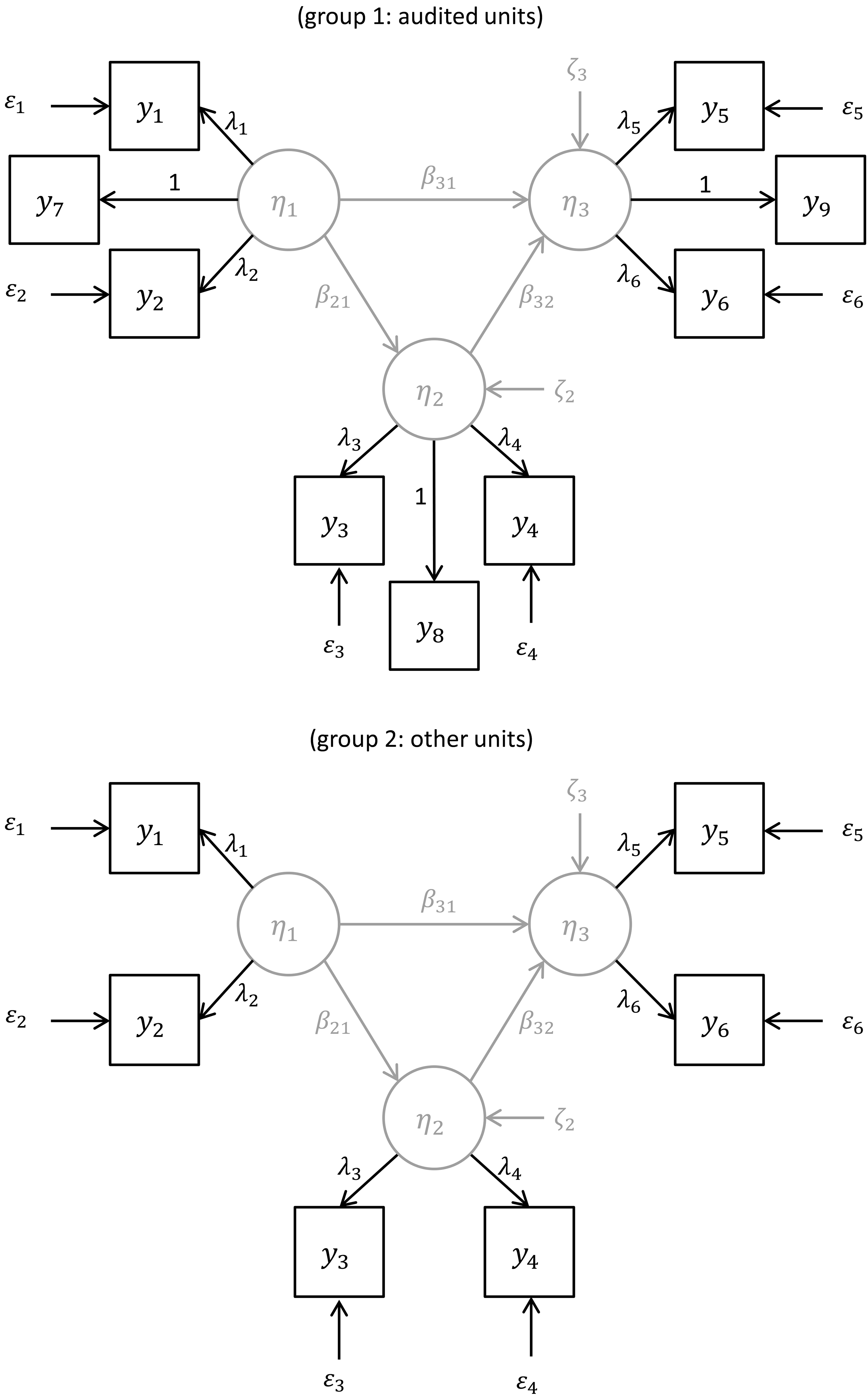
Figure 1 shows an example of an SEM that is identified by means of an audit sample. The model contains three latent variables, each of which is measured by two ordinary, error-prone observed variables. For the units that are selected in the audit sample, additionally observed variables y7, y8 and y9 are obtained that are supposed to measure the latent variables without error. Thus, the measurement equations for these observed variables are simply: y7=η1, y8=η2 and y9=η3. The model is divided into two groups: group 1 represents the audit sample and group 2 the remaining units without additional “gold standard” variables. In group 1, the model is identified by means of the error-free audit data. In group 2, the model is identified by restricting all model parameters in this group to be equal to the corresponding parameters in group 1. This restriction is meaningful, because the audit sample has been selected by random subsampling from the original data set.

In practice, the “gold standard” audit data may be obtained by letting subject-matter experts re-edit a random subset of the original observations. Results on simulated data in [15] suggest that only a small audit sample (say, 50 units) is needed.

An alternative way to identify the model, without the need to collect additional audit data, is to assume that one of the observed variables for each latent variable does not contain systematic measurement errors (while still allowing for random errors). Then the model may be identified by restricting τk= 0 and λk= 1 for these variables. In some cases, this assumption may be reasonable, e.g., for survey variables. However, the assumption cannot be tested with the data at hand (the same holds for the assumption that audit data are error-free).

To estimate the parameters of an SEM, a standard approach is to apply maximum likelihood estimation under the assumption that the data consist of independent, identically distributed observations from a multivariate normal distribution (see [11]). A so-called Robust Maximum Likelihood or Pseudo Maximum Likelihood estimation procedure is available which can handle non-normality of the data as well as complex sampling designs for finite populations (see [16]). Details on how an audit sample can be formally incorporated into this estimation procedure can be found in [14]. Standard fit measures are available to evaluate whether a fitted SEM gives an adequate description of the observed data, and to compare the fit of different SEMs (see [11]).

The validity coefficients VC and the parameters τk and λk provide information about the quality of the input data yk. They can also be used as input to a further procedure to assess the accuracy of output based on these data. As a very simple example, suppose that we are interested in the population mean of the true variable η: θ=(1/N)⁢∑i=1Nηi. Suppose that we have two available estimators:

The measurement model for the observed variables y1 and y2 is given by Eq. (4). Under this model, with the true values ηi treated as fixed, the following expressions can be derived for the mean squared error of the two estimators:

Here, σy⁢12 and σy⁢22 denote the expected population variances of the observed variables under the model. The first terms in the above expression for the mean squared errors are the squares of the corresponding biases, the second terms are the variances.

Thus, in this example the validity coefficients and intercept and slope bias can be used directly to quantify and compare the accuracy of different estimators for the same target parameter. In other situations, it may be too complicated to derive an analytical expression for the mean squared error of a proposed estimator. In that case, the results of the structural equation model could still be used as input for a resampling method (such as the bootstrap) to simulate the effect of measurement errors on the output accuracy.

3.4Variance-covariance matrix for a vector reconciled by means of macro-integration – BDCs 4 and 5 “microdata and aggregated data”

Many statistical figures, for instance in the context of national economic and social accounting systems, are connected by known constraints. We refer to the equations which satisfy such constraints as accounting equations. Insofar as the initial input estimates need to be based on a variety of sources, they usually do not automatically satisfy the set of accounting equations due to the errors of estimates. An adjustment or reconciliation step is required, by which the input estimates are modified to conform to the constraints. Statistical figures sometimes also have to satisfy inequality constraints besides accounting constraints, and input data may need to be adjusted to satisfy these inequality constraints as well. Macro-integration is a technique used for reconciling statistical figures so they satisfy the known constraints.

Consider, for example, an economic model with five macro-economic quantities: national income y, consumption c, investments i, export x, and import m, which are stacked in a vector 𝜷. Suppose that there is one known national accounts identity y=c+i+x-m and one known inequality x⩾m. Given is an initial vector of estimates 𝜷0=(y^0,c^0,i^0,x^0,m^0), where y^0= 600, c^0= 445, i^0= 100, x^0= 515 and m^0= 475. These input data do not satisfy the accounting equations, since 600 ≠ 445 + 100 + 515 - 475. By means of macro-integration the initial estimates can be reconciled so the constraints are satisfied.

Macro-integration can be used to reconcile aggregated data as in the above example. It can also be used to reconcile microdata with aggregated data by first transforming the microdata into estimates on an appropriate aggregated level, for instance by means of weighting these microdata. This approach is, for instance used for the Dutch Population Census (see, e.g. [17, 18]).

[19] considers the following general macro-integr-ation problem

where 𝜷^0 is an unbiased initial vector of estimates for the (numerical) quantities of interest obtained from several data sources with a known (or estimated) variance-covariance matrix V. T and R are matrices and 𝒈 and 𝒉 are vectors defining the constraints that have to be satisfied by the quantities of interest. Problem Eq. (3.4) is a so-called Quadratic Programming problem.

Our aim is to calculate the variance of the vector of estimates 𝜷 after reconciliation. The calculation formula for this variance depends on the type of restrictions that have to be obeyed. Four different cases are distinguished. These cases are discussed below.

3.5Scalar measures of uncertainty in (economic) accounts – BDC 5 “aggregated data”

We again consider accounting systems connected by known constraints. The uncertainty in such an accounting system is, in principle, given by a variance-covariance matrix of all variables involved in the accounting system. However, [21] considers such a system of accounting equations as a single entity and aims to define uncertainty measures that capture the adjustment effect as well as the relative contribution of the various input estimates to the final estimated account in a single scalar. [21] discussed two approaches: the covariance approach and the deviation approach. Below we sketch the covariance approach.

Consider the additive account A=[Y1+…+Yi+…+Yp=Z]. Let Σ𝑿~ be the variance-covariance matrix of the adjusted estimates 𝑿~=(Y~1,…,Y~p⁢Z~). This matrix can be partitioned as follows: Σ𝑿~=(Σ𝒀~Σ𝒀~⁢𝒁~Σ𝒁~⁢𝒀~Σ𝒁~).

One scalar measure, denoted here by γ⁢(A), proposed in [21] is defined as the sum of the variances of the components of 𝑿~, that is

To illustrate the covariance approach let us suppose that we have normally distributed input estimates 𝒀^=(Y^1,…,Y^p)∼Np⁢(𝝁,Σ𝒀), where 𝝁=(μ1,…,μp) and Σ𝒀 is a diagonal matrix with diagonal values σk2=Var⁢(Yk)=σ2⁢μk for k=1,…,p.

Suppose we have an additive accounting equation of the form

where Z~=z is treated as fixed. The original values Y^1,…,Y^p do not necessarily satisfy this accounting equation. Consider a common benchmarking method, which yields the adjusted estimates

where the υk are adjustment weights that sum up to 1 for k=1,…,p. By this benchmarking method the total difference is simply apportioned to each component estimator. Suppose one would like to compare two choices: υk=1/p and υk=μk/∑j=1pμj, which yield, respectively, the adjusted estimates

and

We are interested in which of the two choices, Eq. (10) or Eq. (11), yields statistical data of higher quality. Denote the reconciled estimated account based on Eq. (11) by A1 and the one based on Eq. (11) by A2.

It can be shown (see [21]) that the random variables Y~k-Mk(k=1,…,p) where Mk=E⁢(Y~k)=μk+(z-∑j=1pμj)⁢υk, are negatively correlated with each other and have normal distributions N⁢(0,σ~k2) with

Since Var⁢(Z~)= 0 because Z~=z is fixed, measure γ⁢(A) (see Eq. (9)) is by given by

We examine the difference between γ⁢(A1) and γ⁢(A2). This difference is given by

This implies that γ⁢(A1)⩾γ⁢(A2) with strict inequality unless all μk are equal. So, we conclude that adjustment method Eq. (10) always leads to more uncertainty than method Eq. (11) according to quality measure γ – unless all μk are equal in which case both adjustment methods are equivalent – and that reconciliation method Eq. (11) should therefore be preferred.

3.6Other BDCs

With respect to BDC 3 (“under-coverage”) we have studied extensions of the well-known Petersen capture-recapture estimator (also referred to as the Petersen-Lincoln estimator). This estimator can be used to estimate the size of a population. In the simplest case of this estimator two random samples A and B from the same target population are linked. By n11 we denote the number of units that are observed in both samples A and B, by n10 the number of units that are observed in sample A only, by n01 the number of units that are observed in sample B only, and by n00 the number of population units that are not observed in either of the samples. The unknown population size equals n11+n10+n01+n00. This quantity is unknown since the value of n00 is not observed and unknown. The Petersen estimator for n00 is given by

Its variance (see, e.g., [22]), and hence the variance of the estimator for the population size n11+n10+n01+n^00, is given by

This variance estimate provides a quality measure for the population size estimation. In the literature review we carried out for WP 3, we studied how the Petersen estimator can be applied when the samples A and B are not obtained by survey sampling, but are instead based on administrative data (see, e.g. [23, 24]).

With respect to BDC 6 (“longitudinal data”), we have, for instance, carried out a literature review of [25]. [25] presents an approach to estimate (and possibly correct for) the amount of classification error in longitudinal microdata of categorical variables by estimating a so-called Hidden Markov Model for the underlying “true” distribution. A Hidden Markov Model is a special type of latent class model suitable for longitudinal data. Besides assumptions on the latent class model for each time point also assumptions on the longitudinal structure of the data are needed. In the approach proposed in [25], the true distribution of a categorical target variable, which is measured (with measurement error) for individual units in several linked data sets at several time points, is estimated at each time point. The observed variables are seen as error-prone indicators of a latent true variable, with some assumptions about the distribution of measurement errors. From this, the misclassification rate in each observed variable at each time point can be estimated. The accuracy of observed higher-order properties, such as observed transition rates between categories over time, can be estimated. The approach proposed in [25] can be seen as a longitudinal variation on the approach proposed in [7], which was described in Section 3.2. We refer to [25] for more information about their approach.

References

[1] | Eurostat, European Statistics Code of Practice; 2018, Available at https//ec.europa.eu/eurostat/web/products-catalogues/-/KS-02-18-142. |
[2] | De Waal T, Van Delden A, Scholtus S, Multisource statistics: basic situations and methods. Discussion paper, Statistics Netherlands; (2017) , Available at www.cbs.nl. |
[3] | Van Delden A, Scholtus S, Burger J, Accuracy of mixed-source statistics as affected by classification errors. Journal of Official Statistics (2016) ; 32: (3): 1-25. |
[4] | Meertens QA, Diks CGH, Van den Herik HJ, Takes FW, Data-driven supply-side approach for measuring cross-border internet purchases; (2018) , Available at: arXiv1805.06930v1 [statAP], accessed at 17 May 2018. |
[5] | Van Delden A, Scholtus S, Burger J, Exploring the effect of time-related classification errors on the accuracy of growth rates in business statistics; 2016, Paper presented at the ICES V conference, 21–24 June (2016) , Geneva. |
[6] | Scholtus S, Van Delden A, Burger J, Analytical expressions for the accuracy of growth rates as affected by classification errors; 2017, Deliverable of SGA1 of the ESSnet on Quality of Multisource Statistics. |
[7] | Boeschoten L, Oberski D, De Waal T, Estimating classification error under edit restrictions in combined survey-register data using multiple imputation latent class modelling (MILC), Journal of Official Statistics (2017) ; 33: (4): 921-962. |
[8] | Rubin DB, Multiple imputation for nonresponse in surveys. John Wiley & Sons, New York; (1987) . |
[9] | Arbuckle JL, Full information estimation in the presence of incomplete data. In: Advanced structural equation modeling, (eds). Marcoulides G.A., Schumacker, R.E., Mahwah NJ. Lawrence Erlbaum Associates, Inc.; (1996) , p. 243-277. |
[10] | Van Delden A, Banning R, De Boer A, Pannekoek J, Analysing correspondence between administrative and survey data. Statistical Journal of the IAOS (2016) ; 32: (4): 569-584. |
[11] | Bollen KA, Structural equations with latent variables. John Wiley & Sons, New York; (1989) . |
[12] | Bielby WT, Arbitrary metrics in multiple-indicator models of latent variables. Sociological Methods and Research (1986) ; 15: (1–2): 3-23. |
[13] | Sobel ME, Arminger G, Platonic and operational true scores in covariance structure analysis. Sociological Methods and Research (1986) ; 15: : 44-58. |
[14] | Scholtus S, Bakker BFM, Van Delden A, Modelling measurement error to estimate bias in administrative and survey variables. Discussion Paper 2015-17; (2015) , Available at: wwwcbsnl. |
[15] | Scholtus S, Explicit and implicit calibration of covariance and mean structures. Discussion Paper 2014-09; (2014) , Available at: wwwcbsnl. |
[16] | Muthén BO, Satorra A, Complex sample data in structural equation modeling. Sociological Methodology (1995) ; 25: : 267-316. |
[17] | Houbiers M, Towards a social statistical database and unified estimates at Statistics Netherlands. Journal of Official Statistics (2016) ; 20: (1): 55-75. |
[18] | Knottnerus P, Van Duin C, Variances in repeated weighting with an application to the Dutch labour force survey. Journal of Official Statistics (2006) ; 22: (3): 565-584. |
[19] | Knottnerus P, On new variance approximations for linear models with inequality constraints. Statistica Neerlandica (2016) ; 70: (1): 26-46. |
[20] | Johnson NL, Kotz SN, Balakrishnan N, Continuous univariate distributions Vol. 1. Wiley, New York; (1994) . |
[21] | Mushkudiani N, Pannekoek J, Zhang LC, Uncertainty measures for economic accounts. Deliverable of the ESSnet on Quality of Multisource Statistics; (2017) . |
[22] | Chao A, Pau H-Y, Chiang, S-C, The Petersen-Lincoln estimator and its extension to estimate the size of a shared population. Biometrical Journal (2008) ; 50: (6): 957-970. |
[23] | Gerritse S, Van der Heijden PGM, Bakker BFM, Sensitivity of population size estimation for violating parameter assumptions in log-linear models. Journal of Official Statistics (2015) ; 31: (3): 357-379. |
[24] | Van der Heijden PGM, Smith PA, Cruyff M, Bakker B, An overview of population size estimation where linking registers results in incomplete covariates, with an application to node of transport of serious road casualties. Journal of Official Statistics (2018) ; 34: (1): 239-263. |
[25] | Pavlopoulos D, Vermunt JK, Measuring temporary employment: do survey or register data tell the truth? Survey Methodology (2015) ; 41: (1): 197-214. |