Small area estimation strategy for the 2011 Census in England and Wales

1.Introduction

The key purpose of a census is to produce accurate and reliable estimates of the population, not just at the national level but also, more importantly, for small areas. However, it is widely known that despite all the efforts of the census, some people will be missed [1] and it is standard practice to include an assessment of coverage within the census process. This is usually accomplished through a post-enumeration survey [2]. In the 2001 Census of England and Wales the Office for National Statistics (ONS) re-designed the post-enumeration survey, referred to as the Census Coverage Survey (CCS), to dramatically increase the sample size with a focus on coverage. The result was a large-scale survey designed to provide information that could be matched with the Census in order to estimate directly the age-sex structure of estimation areas (EAs), consisting of populations around 0.5 million individuals [3].

Estimation areas were either a single large local authority (LA) or a contiguous group of smaller local authorities. Local authorities are administrative units of local government and are primarily in charge of key services such as education, housing and social services. At the time of the 2011 Census, there were 348 local authorities in England and Wales and the census is often the main source of information about the population at such small geographies [4]. The same basic census estimation strategy was also implemented for Scotland and Northern Ireland within their estimation area and hard-to-count structures. The units of local administration in Scotland are known as council areas, of which there were 32 for the 2011 Census and in Northern Ireland they are known as districts, of which there were 26 for the 2011 Census. We refer to the ‘UK census’ as shorthand for the censuses in England and Wales, Scotland and Northern Ireland.

Population size and structure are key drivers in the allocation of funding to local authorities from central government. Hence it is important that the census counts are adjusted for the estimated undercount to enable a fair and accurate allocation of resources. To facilitate this, the ideal would be a CCS designed to estimate the coverage of the age-sex population directly at local authority level. However, like any other national statistical institute, the Office for National Statistics faces the challenge of producing comprehensive, accurate and reliable information in a timely and cost-efficient manner. A CCS with sufficient sample size for direct estimation of all local authorities would not only increase costs, but its size would potentially reduce the overall quality, as undertaking such a large data collection exercise very close to the census would be problematic. Therefore, it is necessary to turn to small area techniques [5] that allow the age-sex estimates for an individual local authority to borrow strength from neighbouring local authorities or neighbouring age-sex categories within the local authority, while still attempting to reflect localised effects. In general, direct estimators (based only on the small CCS sample from within a local authority) will be unbiased, but have large standard errors and so are imprecise. On the other hand, indirect methods, although more precise, can have large biases [6, 7]. For the 2001 Census, borrowing strength was achieved with the inclusion of local authority specific fixed-effects within a collapsed version of the main estimation model used for estimation areas. Such an approach combined direct information from the specific local authority with pooled information across the local authorities within their estimation area.

Following reviews of the 2001 Census adjustment approach (see [8, 9]), the Office for National Statistics adopted broadly the same strategy for the 2011 Census [2]. However, the 2001 Census provided substantially more data from which to develop the 2011 approach. This led to a change in the CCS design structure so that allocation to local authorities was directly controlled in the design, stratification within local authorities was based on more up-to-date information on the population structure and the allocation was driven by variation in coverage patterns observed in 2001 [10]. The result is that many of the city local authorities, Coventry for example, that did not have a big enough population to count as an estimation area in 2001 are a single local authority estimation area in the 2011 design. Conversely, the estimation areas that are aggregates of local authorities tend to contain more local authorities than in 2001 but with a stronger expectation that within estimation area homogeneity across the local authorities can be achieved during assessment [11]. First, this was because the estimation areas are formed after the design stage so local authorities can be aggregated, albeit still reflecting geographical contiguity, to take account of the observed patterns in coverage from 2001. Second, the move to mailing and receiving census forms to households (post-out/post-back) combined with flexible allocation of staff for non-response follow-up was expected to smooth out census coverage patterns across local geography more than was seen in 2001 [12]. Therefore, in this paper we outline the development of the strategy for applying small area techniques to produce local authority population estimates for the 2011 census in the light of the updated design of the CCS [10] and the overall estimation strategy for the estimation area level. The discussion focuses on the small area estimation strategy to provide local authority estimates. Interested readers can refer to the partner paper [11] which provides the background, context and details of the coverage assessment process of the 2011 census.

2.Census Coverage Survey (CCS) Design and Estimation for the 2011 Census

The output from the census coverage adjustment process is a complete database with individual and household level records for the entire population, taking full account of any estimated under-coverage. The process begins with the census, which attempts to enumerate the whole population. This is followed by the CCS which undertakes an intensive re-enumeration of a sample of the population. The CCS is a nationally representative sample of over 300,000 households (grouped into postcodes, which are small geographical units made up of 15 to 20 households) and the design is described in [10]. The CCS responding households are matched to the census responses and, for the sampled postcodes, estimates of the missed households and persons are calculated through the application of dual-system estimation [13]. The dual-system estimates are used as inputs to a ratio estimation using census counts as an auxiliary variable to produce estimates of the population for estimation areas. Where an estimation area consists of more than one local authority the estimation area totals then need to be allocated to the constituent local authorities through small area techniques. There are additional stages in the census coverage process, such as quality assurance using administrative datasets and demographic analysis, which often involve inspecting the implied sex ratios of the population as well as birth and death rates. The resulting local authority level estimates are used as control totals for the imputation system that produces the fully adjusted database, as outlined in [14]. This paper focuses on the small area estimation part of the coverage process and complements [11] which describes the framework for estimation at the estimation area level.

The small area approach outlined here builds on the approach used in 2001 accommodating for the adjustments to the CCS design for 2011 outlined in [10]. The CCS design in 2001 created estimation areas by grouping contiguous local authorities together with the aim of having a population of around 0.5 million. This was done at the design stage and then there was a further stratification by a Hard-to-Count index before allocating the sample [3]. Local authorities were not explicitly accounted for in the design, and there was no historical data to provide evidence of variation in census coverage to drive the formation of the estimation areas. Therefore, it was important that the small area technique used could directly reflect local authority specific variation in coverage remaining after controlling for age-sex and Hard-to-Count index at the estimation stage.

The small area level estimates are contingent on the results of the dual-system estimation, which in turn are reliant on the accuracy of the matching of the census and the CCS. This matching process produces a contingency table with the number of individuals that were in both the census and CCS (n11), in the census but not in the CCS (n10) and those not in the census but in the CCS (n01). By definition, the individuals that are counted neither by the census nor CCS (n00) are unknown, and are referred to as the undercount. In order to estimate the total population it is required to adjust for this undercount by finding an estimate of those missed by both the census and CCS. This is achieved through the assumption that there is independence between the census and CCS. Thus the estimate of those missed by both the census and CCS can be found by the expression

Dual-system estimation also relies on the assumption that individuals have the same chance of being counted by either the census or CCS. Here, the homogeneity assumption does not hold across the entire population, unless the population is subdivided into groups of similar individuals through post-stratification [13]. In the UK, this is achieved firstly by dividing the country broadly along regional lines into estimation areas. If the local authority is particularly large – for example Manchester – the local authority comprises an estimation area of its own. On the other hand, London has several estimation areas based on grouping contiguous local authorities within the metropolitan area.

The population is further stratified by age and sex, and a ‘hard-to-count’ index. The 2001 Hard-to-Count index (see [3]) was constructed from household characteristics known to be associated with under-coverage, such as high levels of multi-occupancy and private rented accommodation, based on information from previous censuses and social surveys. It had three strata – easy, medium and hard – and it was assumed that post-stratification using age, sex and Hard-to-Count index gave reasonable assurance that within each post-stratum there was homogeneity of being counted in the census or CCS (For the 2011 census the Hard-to-Count index described by [12] was extended to five strata). Then for each of the post-strata, those missed in both the census and CCS (n00) can be reasonably estimated with the dual-system estimator (DSE). The dual-system estimator is applied at low levels of geography consisting of three to five postcodes, which provide sufficient data to yield stable estimates as well as forming the primary sampling unit for the design of the CCS [10].

It is possible to produce direct estimates of the local authority totals based on information from the CCS. However, these have unacceptably large standard errors due to small sample sizes, particularly after stratifying by the CCS design variables (such as age and sex). Sample sizes for the local authorities are small partly to keep the survey manageable, and also because the overall sample size was determined to provide specific accuracy at the estimation area level. Research was carried out to ascertain if it were possible to increase the sample size in order to facilitate direct estimation of the local authority totals from the CCS. However, this was deemed not feasible [10]. The CCS, in addition to being nationally representative, is already a large survey. It is eight times the size of the quarterly Labour Force Survey, which has a responding sample of approximately 40,000 households per quarter [15].

Indirect estimates of the small area population can be produced which increase the effective sample sizes of the local authorities using information from related areas and thereby reducing standard errors. The drawback of these indirect techniques, however, is that they rely on strong assumptions about the relationship between the small areas themselves, in addition to the relationship between the small area and the larger area. Thus, while the estimators may have low variances, they tend to be biased. Therefore, the small area strategy has to strike a balance between the potential bias of an indirect estimator and the imprecision of the direct estimator.

In 2001 a number of different approaches were considered on the basis of available literature and the suitability of the underpinning model assumptions. The small area models were then assessed to find the model that was capable of delivering accurate estimates of the population under various coverage scenarios. In the final model selected, information from all the local authorities within an estimation area was used to model the undercount, but the model coefficients (i.e. the slopes of the regression lines) were allowed to vary by local authority. As a consequence, the heterogeneity of the slopes accounted for the differences in coverage between local authorities and within the specific estimation area [16].

3.Small area estimation for local authorities in the 2011 Census

The main objective of the small area estimation strategy is to produce reliable population estimates, with corresponding precision measures, by Hard-to-Count index strata and age-sex groups within each local authority. The age-sex categories used were similar to those used in 2001. There were 35 age-sex groups given by males and females under 1 year old, males from 1 to 4 years old, females 1 to 4 years old, then 5 year age groups for males and for females up to 79 years old, males over 80 years old and females over 80 years old. The small area estimation procedure implemented for the 2011 census apportions the estimation area estimates to the local authorities by assuming a relationship between the undercount pattern at the local authority (small area) level and the broader area (i.e. the estimation area). The starting point is a local authority by Hard-to-Count index strata age-sex specific model and we then explore how to estimate that model by borrowing strength in various dimensions.

To specify a model we start by defining some notation using the same structure as [11]. We assume that modelling takes place within an estimation area, and drop any subscript to distinguish estimation areas (although we use a subscript e to show statistics calculated over the whole estimation area). Let Yo⁢a be the true count for age-sex group a, from the sampled postcodes in output area o. Within each stratum h, the counts are assumed to be homogenous. In our application these homogenous strata formed as a combination of the Hard-to-Count index strata by each local authority, and we denote this as HtC-within-LA stratum. In reality, this is the dual-system estimate (see [11]) at the cluster level combining across sampled postcodes within output area. Also, let Xo⁢a be the corresponding unadjusted census count. A simple model that links the true counts to the census counts as an auxiliary is the ratio model

It is essentially a set of independent ratio models for each age-sex group by HtC-within-LA strata, i.e., with ratios Rh⁢a at the level of the individual local authority.

An optimal estimator for Eq. (3) follows from [17] and uses the weighted least squares estimator for Rh⁢a given by

where Yo⁢a, the sum across the sampled postcodes in output area o, is then replaced by the cluster level dual-system estimator and sh represents the output areas sampled from the HtC-within-LA strata h. An estimator of the total is then given by T^h⁢a=R^h⁢a⁢Xh⁢a. This is just applying the ratio adjustment to the total unadjusted census count; or more correctly it sums the estimated true counts, observed for the sample data, and then predicts using the estimated ratio applied to the unadjusted census counts for the non-sampled postcodes. This is the model and estimator that is used for an estimation area containing a single local authority with the Y’s replaced with cluster level dual-system estimates to estimate the individual ratios. We now explore ways to ‘borrow strength’ to estimate the population size for local authorities when the sample size is too small to support directly estimating model Eq. (3).

Various regression type models that collapsed Eq. (3) across different dimensions were considered in a simulation study with the objective of finding an estimator that balanced the trade-off between variance and bias, yielding estimates with good precision and as little bias as possible. As the CCS was stratified by the Hard-to-Count index, and this was expected to be a good proxy for variation in census coverage, the small area models produce Hard-to-Count-specific estimates of the local authority population totals. The general objective is, therefore, to produce model-based estimators for the population total by HtC-within-LA stratum and age-sex group, T^h⁢a. Here we focus on three alternatives: one direct estimator and two indirect estimators. In the 2001 Census, and again in 2011, the final model-based estimates T^h⁢a were scaled to the estimation area age-sex population total. This calibration ensured that estimates produced by the small area modelling would be consistent with the sub-national and national population estimates. Variance estimation for the local authority estimates within an estimation area was undertaken using a bootstrap approach developed by [18] in application to population total estimation with a finite sampling population correction (see Chapter 5 of [19]) to ensure that the lower level local authority estimates aligned to the (higher-level) estimation area estimates.

4.Evaluation of the small area methods

The relative performance of the three estimators depends on the strength of localised census enumeration effects that cannot be controlled for using a combination of age-sex and Hard-to-Count classifiers within an estimation area. To get an idea of the trade-offs in these different effects, a simulation study was used to evaluate the three competing estimators. A series of censuses and CCSs were simulated using predicted coverage probabilities obtained through modelling of the under coverage in the 2001 census and CCS data. Simulations were produced for a number of estimation areas with a variety of coverage patterns. For each estimation area in the simulation, 400 censuses and 400 CCSs were used. The first step in the estimation procedure was to produce estimates of the population totals for the larger domains, here the estimation areas. For each simulated census and CCS combination, dual-system estimation and ratio estimation were used to produce estimates of the estimation area totals for the detailed age-sex groups by hard-to-count stratum. After this was completed, the local authority estimates by age-sex group and Hard-to-Count stratum were obtained for each of the 400 simulations within an estimation area using the three competing estimators.

As outlined in Section 2, the indirect estimators have a tendency to be biased in comparison with the direct estimators. The aim of the evaluation process was to weigh the reduction in variance against potentially larger biases. Therefore, based on the 400 simulation results the relative bias and the relative root mean squared error were calculated as suitable measures of performance that could be used to investigate the bias and variance. The mean squared error is a function of both the variance and bias, and is consequently a good measure of the overall accuracy of the different estimators (see page 253 of [20]). The relative root mean squared error (RRMSE) and the relative bias (RB) for each domain (HtC by age-sex classification) in a given local authority are respectively calculated as

where:

Th⁢a is the true population count for the age-sex group a in HtC-within-LA stratum h; and T^h⁢a(j) is the corresponding model based population estimate obtained from the jth simulation, with j=1,…,400.

4.1Results of the simulations

Simulated census and CCS data were obtained for some estimation areas which were selected because they had different levels of coverage in the 2001 census. As the investigation sought to determine how each of the different small area models fared under a range of coverage scenarios, estimation areas were chosen to exhibit diverse census coverage characteristics. This paper presents results from four estimation areas to show the methodological development of the small area strategy for the 2011 UK census. The chosen areas are KK and KO from the Midlands, LB from Inner London, and LJ from Outer London, which cover a range of observed census coverage patterns for the 2001 Census. These pseudonyms (KK, KO, LB, and LJ) are used to protect the confidentiality of the estimation areas (and related local authorities). These estimation areas consist of two or three constituent local authorities and showcase the issues that had to be considered when choosing a suitable small area methodology to produce reliable estimates of the local authority totals.

Table 1 gives the 2001 Census coverage rates by local authority and estimation area. It shows that higher coverage is achieved in KK and KO but lower coverage in LB and LJ. In addition, there are some differences in coverage by local authority within estimation areas reflecting the fact that 2001 estimation areas were based on geography and population size with little available evidence relating to localised variation in census coverage. However, this variation may also be related to differing age-sex and Hard-to-Count structures within the local authorities of each estimation area.

For each of the estimation areas, the RRMSEs and RBs were calculated for the three competing small area estimation techniques (namely direct estimatorT^h⁢a𝑑𝑖𝑟, synthetic estimatorT^h⁢a𝑠𝑦𝑛𝑡ℎ and local fixed effects model estimatorT^h⁢a𝐿𝐹𝐸). We were interested in exploring the behaviour of the different small area estimators and to determine which estimator produced the most robust estimates of the local authority population totals. Table 1 shows the RRMSE and RB for the local authority population totals in each estimation area. The results in the table for the three small area model-based estimates were found by summing across the age-sex groups and the hard-to-count strata. This gave an indication of the variability of the different local authority population totals produced by the different small area strategies. From Table 1, when the target parameter is the local authority population total, the synthetic estimator produced the lowest RRMSE in five of the 11 local authorities; and was very similar to the lowest in a further three. The estimates where it is lowest all occur in the two London estimation areas where the observed coverage patterns for the local authorities in the 2001 Census were relatively similar within each estimation area. The local fixed effects model estimator was also the lowest in five local authorities and these occur in the other two estimation areas which tend to have higher coverage but greater variation across the local authorities within each of the estimation areas.

In terms of RRMSE, the choice is between a synthetic estimator that is likely to have smaller variance but more potential for bias and local fixed effects model estimator with potentially higher variance but less bias. This was confirmed by the bias results in Table 1, where the synthetic estimator typically has larger absolute bias with either the local fixed effects model or direct estimator having the smaller absolute biases. However, it is worth noting that in the design for the 2011 CCS [10], the direct use of local authority in the design results in KK1, KO1 and all of LB being treated as estimation areas with a single local authority at estimation [11] due to their more extreme coverage patterns relative to neighbouring local authorities. Therefore, taking the results in Table 1 with the changing structure of the CCS, the synthetic estimator would be expected to perform better in terms of RRMSE but there may be a small bias if the estimation areas combine local authorities that then experience localised coverage effects in 2011.

While Table 1 presents results for the total population, it is important to consider the age-sex by Hard-to-Count estimates as this is the level at which the estimators operate. Boxplots of the distributions of RRMSEs and RBs for the 105 (i.e. 35 × 3) age-sex by Hard-to-Count model-based population estimates for each local authority are shown in Fig. 1. Small area techniques that perform well should produce an RRMSE distribution with lower median and a smaller spread. In the case of bias, a good technique should produce an RB distribution that is centred around zero with small spread. For both RB and RRMSE distributions outliers are indicative of possible model failure, therefore any outlying observations are highlighted in the boxplots.

Figure 1.

Boxplots showing the RB and RMSE distribution of the different small area estimators for the selected four estimation areas. For each plot the left panel represents the direct estimator, middle panel represents the synthetic estimator, and the right panel represents the local fixed effects model.

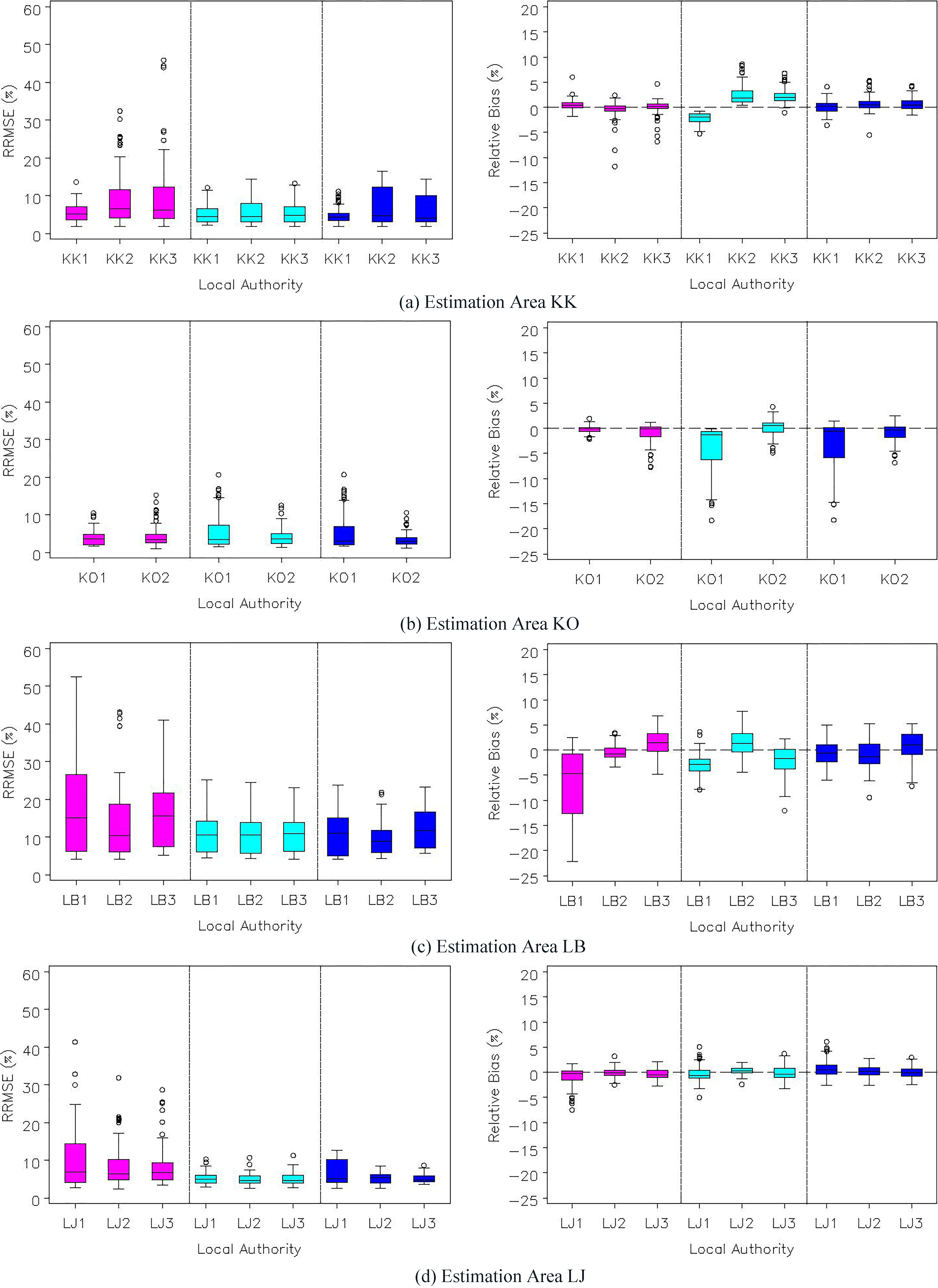
The boxplots for the estimation areas KO, KK, and LJ are less skewed and exhibit smaller variability in comparison to LB. These boxplots provide evidence that in general the synthetic estimator has lower RRMSEs and performs best in comparison to the local fixed model and the direct estimator. Furthermore, the distributions have smaller spread within local authorities for each of the estimation areas. However, when examining the relative biases, the local fixed effects model produces better behaved distributions, which are mostly centred around zero and are therefore approximately unbiased. The reasoning behind the local fixed effects estimator is to capture any difference in coverage due to local authority effects. Although no improvement in the RRMSE was found, the model containing local authority effects may protect the estimation procedure against failure when local authority differentials are observed. This motivated the use of the local fixed effects model in estimation areas where there was evidence of coverage variation between local authorities within the estimation areas.

The analysis shows that the synthetic estimator has the best overall performance. An explanation of why the synthetic estimator does better than the local fixed effects estimator is simply that the simpler model behind the estimator is sufficient to capture the likely coverage patterns. The local fixed effects model includes a fixed effect for each local authority, however if there are no (or only small) local authority differentials in undercoverage, then additional modelling error is being introduced, with little benefit. Furthermore, the results do make some sense in the context of the coverage rates in Table 1. Most of the local authorities have similar coverage rates to the overall estimation area coverage. Even in estimation areas with relatively poor coverage, such as the inner London boroughs of LB, all the local authorities exhibit similar coverage patterns. The local fixed effects model is useful when the different local authorities in the estimation area have varying coverage rates. Additionally, the local fixed effects model has some definite benefits with regards to its intuitive appeal: it can offer more protection against model failure than the synthetic estimator. Notice that the direct estimator, which is typically less efficient than the synthetic and local fixed model estimators since it does not borrow strength outside the estimation domain, still performs well; and can perform as well as the other two estimators, as is evidenced in KO.

Table 2

A comparison of model ‘goodness of fit’ for estimation areas and hard to count strata where the BIC (Schwarz Bayesian Information Criterion) goodness of fit measure for the fixed effects model is smaller than that for the synthetic models

EA code	Hard-to-Count	Number	Fixed effects –		Synthetic model –		Synthetic model –
	stratum	of LAs	collapsed age-sex groups		collapsed age-sex groups		full age-sex groups
			BIC	AdjR2	BIC	AdjR2	BIC	AdjR2
EE05	1	6	- 996.9	0.9855	- 957.1	0.9834	- 897.2	0.9833
	2	7	-1712.0	0.9892	-1748.5	0.9893	-1681.8	0.9892
SE03	2	3	-1268.2	0.9858	-1270.4	0.9856	-1220.91	0.9855
	3	2	- 402.4	0.9776	- 376.2	0.9752	- 326.4	0.9745
SW04	1	3	-441.4	0.9850	-450.2	0.9850	-401.5	0.9846
	2	3	- 681.6	0.9845	- 664.8	0.9833	- 608.8	0.9829
	3	2	- 38.9	0.9368	- 37.8	0.9345	8.9	0.9305
WA02	1	3	- 1098.7	0.9775	- 1093.0	0.9769	- 1024.6	0.9766
	2	3	-466.8	0.9750	-472.0	0.9747	-420.1	0.9746
WM03	2	2	-1436.4	0.9809	-1441.6	0.9808	-1366.8	0.9806
	3	2	- 304.5	0.9449	- 303.1	0.9441	- 241.1	0.9437
YH07	1	2	- 719.3	0.9953	- 713.6	0.9951	- 665.7	0.9950
	2	2	-1417.3	0.9839	-1423.9	0.9839	-1361.4	0.9837

The results indicate that both the synthetic estimator and local fixed effects model estimator are reasonable options to produce local authority population estimates. The first performs better in terms of RRMSE whereas the latter produces estimates with smaller biases. The synthetic estimator, however, seems more stable as it shows less variability in performance across local authorities (as shown earlier in Fig. 1). The use of a local fixed effects model could represent a safeguard for local authority undercoverage differentials. However, as demonstrated in some of the results, the local fixed effects model may add unnecessary noise into the estimates if there are no local authority effects to be observed. The compromise solution for the 2011 census was to implement a small area estimation procedure that accommodated both options. That is, the synthetic estimator was the default option for each estimation area, thereby assuming the local authority effects were not important. Then, if the quality assurance procedure found evidence of a localised failure in coverage, fit a local fixed effects model and test the significance of the areal effects.

4.2Assessing the Performance in 2011

Based on the simulation results and the change in structure to the CCS, the standard approach implemented in the 2011 Census utilised synthetic estimation for local authorities within an estimation area. The use of local fixed effects would be explored only if quality assurance identified evidence of localised coverage effects that needed to be accounted for. No such situations occurred, so all local authority outputs were either for a single local authority making up an estimation area by itself, or synthetic estimates within the estimation area. However, we can now explore the models in a little more detail to assess the robustness of this approach using the actual 2011 data.

For the 70 estimation areas that contain more than a single local authority, we compare the synthetic model with the full set of age-sex categories to a synthetic model with the collapsed age-sex categories and then the local fixed effects model (with the same collapsed age-sex categories). Having the synthetic approach for both the full and collapsed age-sex groups allows us to assess the cost of reducing the number of groups prior to assessing the potential benefit of adding the local fixed effects. The approach used to assess the strength of the local authority effects in a given estimation area was to compare the different models using two goodness-of-fit measures: the Schwarz Bayesian Information Criterion (BIC) and the adjusted R2 value. In both cases the measures are based on the variation explained by the model but with penalties for the number of parameters, making them suitable to compare non-nested models. In the case of the BIC smaller values represent better fit, while for the adjusted R2 larger values imply better fit.

The BIC for the local fixed effects model was found to be smaller than that for either of the synthetic models in just six of the 70 estimation areas considered. This indicates that for the vast majority of estimation areas there was no evidence of strong local authority effects. The six estimation areas where there was some indication of stronger local authority effects were examined in greater detail. The model goodness of fit statistics for these estimation areas are given in Table 2.

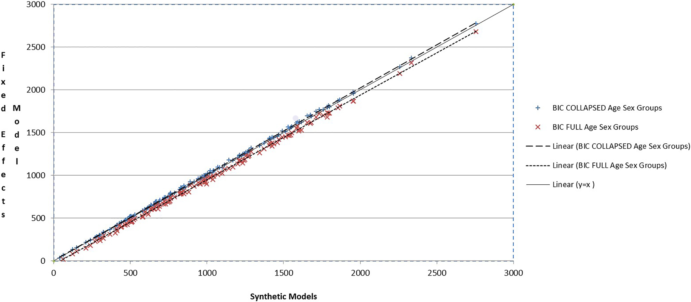
Figure 2.

Schwarz Bayesian Information Criterion (BIC*) values for fixed effects models against synthetic models. *The BIC values have been multiplied by -1 so that in this figure the larger the BIC value the better.

In all but one of these six estimation areas in Table 2, just one of the Hard-to-Count strata had the smallest BIC for the local fixed effects model. The exception is the estimation area coded SW04 from the South-West, where both hard to count strata 2 and 3 have smaller BIC values for the local fixed effects models. In Table 2 it can also be seen that the difference in BIC values between the local fixed effects model and the collapsed age-sex group synthetic model is small for these six areas, regardless of which model has the actual lowest value. This implies that the addition of fixed effects over broader age-sex groups has little advantage. The BIC values for both the collapsed age-sex group local fixed effects model and the collapsed age-sex group synthetic model are smaller than the corresponding values for the full age-sex group synthetic model. This implies there is some potential efficiency gain from collapsing age-sex groups, but the requirement to produce estimates for the five-year age-sex groups means we would not want to collapse unless it was needed to allow the inclusion of the local fixed effects. The adjusted R2 values are generally largest for the local fixed effects model, but there is little improvement in the adjusted R2 from including the local authority effects or collapsing the age-sex groups.

In Fig. 2 the BIC values for all areas obtained from fitting both synthetic models are plotted against the BIC value from the corresponding local fixed effects model, together with the fitted lines. Also plotted is the y = x line to demonstrate how close the values from the synthetic models are to the local fixed effects model. In this figure the signs of BIC values have been changed so that the larger the BIC value the better. In Fig. 2, the fitted line of the local fixed effects against synthetic with collapsed age-sex groups is very close to the y = x line showing, in general, that adding the local authority effects does not improve the fit of the model compared to a synthetic model with the same age-sex groups. However, the fitted line for the SBC values from the comparison of local fixed effects to the synthetic model with the full age-sex categories is slightly below the y = x line, which indicates that having a greater number of age-sex groups in the model generally results in an improved fit over the inclusion of the local authority effects and a reduced age-sex categorisation. From these overall results in Fig. 2, combined with the small number of estimation areas highlighted in Table 2, we can see that the small area strategy for 2011 performed well in that the synthetic approach did well in the vast majority of cases. Even when the local fixed effects model gave an improved fit, the gain was marginal; and this shows why these impacts were not detected in the quality assurance process.

5.Conclusions

Small area estimation techniques are useful in overcoming the problem of small sample sizes since direct estimates using data from the CCS would have correspondingly large standard errors and be imprecise. However, although they are precise, these (indirect) model based estimators may be more biased than the direct estimators. Therefore, the aim of the evaluation of different estimators was to balance the trade-off between variance and bias in order to find the estimator that produced estimates with good precision and as little bias as possible. The small area models work by incorporating auxiliary information by assuming relationships between the undercount pattern in the local authority and broader areas such as the estimation area. The underlying idea was to exploit the similarities in the undercount patterns so as to borrow strength over the areas through the use of regression models relating the dual-system estimates to the census counts.

The main reason for using indirect estimation for the local authority population totals is to improve precision by combining information from the broader estimation area to increase the effective sample size. In this paper we explored two indirect approaches, the synthetic estimator and local fixed effects estimator, both applied within an estimation area. In preparation for the 2011 Census, additional research was carried-out to assess more complex indirect estimators based on models using random effects but fitted to larger areas, in our case government office region (GOR). The underlying assumption here was that the undercount pattern in the government office region was similar to the undercount pattern in the local authority. Obviously, this is not necessarily true but the inclusion of random effects helps account for local authority differentials in (non)response. In addition, we considered composite models which took a weighted combination of the synthetic estimator and the local fixed model. These composite estimators tended to increase the variability and were found to be inefficient.

The recommendation is to accommodate both synthetic estimation and local fixed effects regression. The synthetic estimator was the default technique, and could cope with some local authority differentials provided they could be explained by hard-to-count and age-sex patterns. However, in the case that there were unanticipated problems in the census and the CCS leading to greater differences in the observed local authority coverage levels, this would be detected by the quality assurance process and the local fixed model would be better placed to produce more robust population estimates.

During the estimation for the 2011 Census, the quality assurance did not trigger the use of local fixed effects, as the default synthetic estimates were accepted. However, here we present the results from a modelling exercise that compared the two approaches for all 70 estimation areas. The results of this confirm that the synthetic model was generally a better fit than the local fixed effects model. However, it also highlighted how little difference there was between the approaches which all had very high values for the adjusted R2 showing how well the models explained the variation in coverage using the census counts. This demonstrates that an initial population count that manages to count everyone well, with very little undercount, will ensure a more robust small area adjustment with accurate local authority population estimates. Conversely, any small area technique will struggle to adjust a poorly performing census. Looking ahead for the next censuses in 2021 and beyond, the small area estimation strategy can be enhanced with the use of administrative register data, specifically during the final quality assurance of the estimates, to ensure more robust and reliable adjusted population counts at a local authority level.

References

[1] | Diamond I. The Census. In: Dorling D, Simpson L, eds. Statistics in Society: the arithmetic of politics. London: Arnold; (1999) ; pp. 9-18. |
[2] | Abbott O. 2011 UK Census Coverage Assessment and Adjustment Methodology. Population Trends (2009) ; 137: : 25-32. |
[3] | Brown JJ, Diamond ID, Chambers RL, Buckner LJ, Teague AD. A methodological strategy for a one-number census in UK. Journal of the Royal Statistical Society: Series A (1999) ; 162: : 247-267. |
[4] | Rao JNK, Molina I. Small area estimation, 2 |
[5] | Martin D. Editorial: census present and future. Journal of the Royal Statistical Society: Series A (2007) ; 170: : 263-266. |
[6] | Pfeffermann D. Small area estimation – new developments and directions. International Statistical Review (2002) ; 70: : 125-143. |
[7] | Ghosh M, Rao JNK. Small area estimation: an appraisal. Statistical Science (1994) ; 9: : 55-93. |
[8] | Office for National Statistics. 2001 census: Manchester and Westminster matching studies full report. London: Office for National Statistics (2004) [cited 2017 Oct 19]. Available from http://www.ons.gov.uk/ons/guide-method/method-quality/specific/population-and-migration/pop-ests/local-authority-population-studies/2001-census—manchester-and-westminster-matching-studies-full-report.pdf. |
[9] | Local Government Association. The 2001 One Number Census and its quality assurance: a review. Research Briefing 6.03. London: Local Government Association; (2003) . |
[10] | Brown J, Abbott O, Smith PA. Design of the 2001 and 2011 census coverage surveys for England and Wales. Journal of the Royal Statistical Society Series A (2011) ; 174: : 881-906. |
[11] | Brown J, Sexton C, Abbott O, Smith PA. The framework for estimating coverage in the 2011 Census of England and Wales: combining dual-system estimation with ratio estimation. Submitted to Statistical Journal of the International Association of Official Statistics; (2017) . |
[12] | Abbott O, Compton G. Counting and estimating hard-to-survey populations in the 2011 Census. In: Tourangeau R, Edwards B, Johnson TP, Wolter KM, Bates NA, eds. Hard-to-Survey Populations. Cambridge: Cambridge University Press; (2014) . |
[13] | Sekar CC, Deming WE. On a method of estimating birth and death rates and the extent of registration. Journal of the American Statistical Association (1949) ; 44: : 101-115. |
[14] | Steele F, Brown J, Chambers R. A controlled donor imputation system for a one-number census. Journal of the Royal Statistical Society, Series A (2002) ; 165: : 495-522. |
[15] | Office for National Statistics. Quality and methodology information (LFS). Information Paper. Newport: Office for National Statistics; (2015) . |
[16] | Office for National Statistics. One number census local authority estimation. London: Office for National Statistics; (2000) [cited 2017 Oct 19]. Available from http://www.ons.gov.uk/ons/guide-method/census/census-2001/design-and-conduct/the-one-number-census/methodology/steering-committee/key-papers/local-authority-estimation.pdf. |
[17] | Royall RM. On finite population sampling under certain linear regression models. Biometrika (1970) ; 57: : 377-387. |
[18] | Efron B, Tibshirani RJ. An introduction to the bootstrap. Boca Raton: Chapman & Hall/CRC; (1993) . |
[19] | Wolter K. Introduction to variance estimation. 2 |
[20] | Cox DR, Hinkley DV. Theoretical statistics. London: Chapman and Hall; (1974) . |