
The framework for estimating coverage in the 2011 Census of England and Wales: Combining dual-system estimation with ratio estimation
Abstract
Dual-system estimation is a well-established approach for estimating an unknown population size from two independent but imperfect counts of the population. In this paper we develop the estimation framework for using a coverage survey and population census as the two sources and combining with ratio estimation to produce a set of population estimates. Adjustments are developed to correct for a failure of the key assumptions of homogeneity and independence that under-pin dual-system estimation using an external count of the number of households. The issue of over-count within the census is also discussed and a bootstrap approach to variance estimation is proposed. A comprehensive set of simulation results are presented to support the decision to implement the framework to estimate the population following the 2011 Census of England and Wales; and the implementation to the estimation of census coverage in 2011 is discussed.
1.Introduction
The failure of the 1991 Census Validation Survey to correctly estimate the level of census under-coverage is well documented [1, 2]. This led to re-thinking the approach to coverage assessment for the 2001 Census. The result was the one-number census project, with the goal of accurately measuring and adjusting for census coverage issues. A key component of the one-number census was a large-scale, independent post-enumeration survey called the Census Coverage Survey (CCS). The early thinking on the design of the CCS and the approach to estimation were outlined in [3] while the development of the imputation system to adjust the database was covered in [4]. Adjustments to the key age-sex estimates were detailed by [5].
Evaluating the census age-sex estimates for coverage is standard practice and was recommended by the United Nations (UN) for the 2010 round of population and housing censuses [6]. The imputation for unit non-response (households and people) carried out in the UK in 2001 is unique, although a similar approach was planned for the 2000 Census in the US (see [7]). In particular, the US Census Bureau has a long history of assessing census coverage using a survey, dating back to the 1950 Census [8], although the alternative estimates produced in [9] show that estimating census coverage has always been difficult. Starting with analysis post 1980 [10, 11], followed by developments at subsequent censuses, the Bureau’s primary approach is now based on dual-system estimation [12] with a large national post-enumeration survey [13, 14, 15, 16]. The Australian Bureau of Statistics also developed an estimation approach to combine its census with a survey during the 1980s and the current implementation for 2011 is developed and discussed in [17, 18]. Other examples include the approach used for the 2000 Census of Switzerland, as outlined in [19], and for Israel, as outlined in [20]. Many of these approaches are loosely based on the US Census Bureau application and this is the UN’s recommended approach, outlined in [6], and therefore widely adopted by countries in the 2010 round of censuses. A different approach, the reverse record check, was developed by Statistics Canada, utilising historical census data matched with other administrative data to estimate coverage of the current census. A description of the methodology can be found in [21], and Statistics Canada continue to take advantage of additional administrative data sources to assist in tracing of persons in the reverse record check sample.
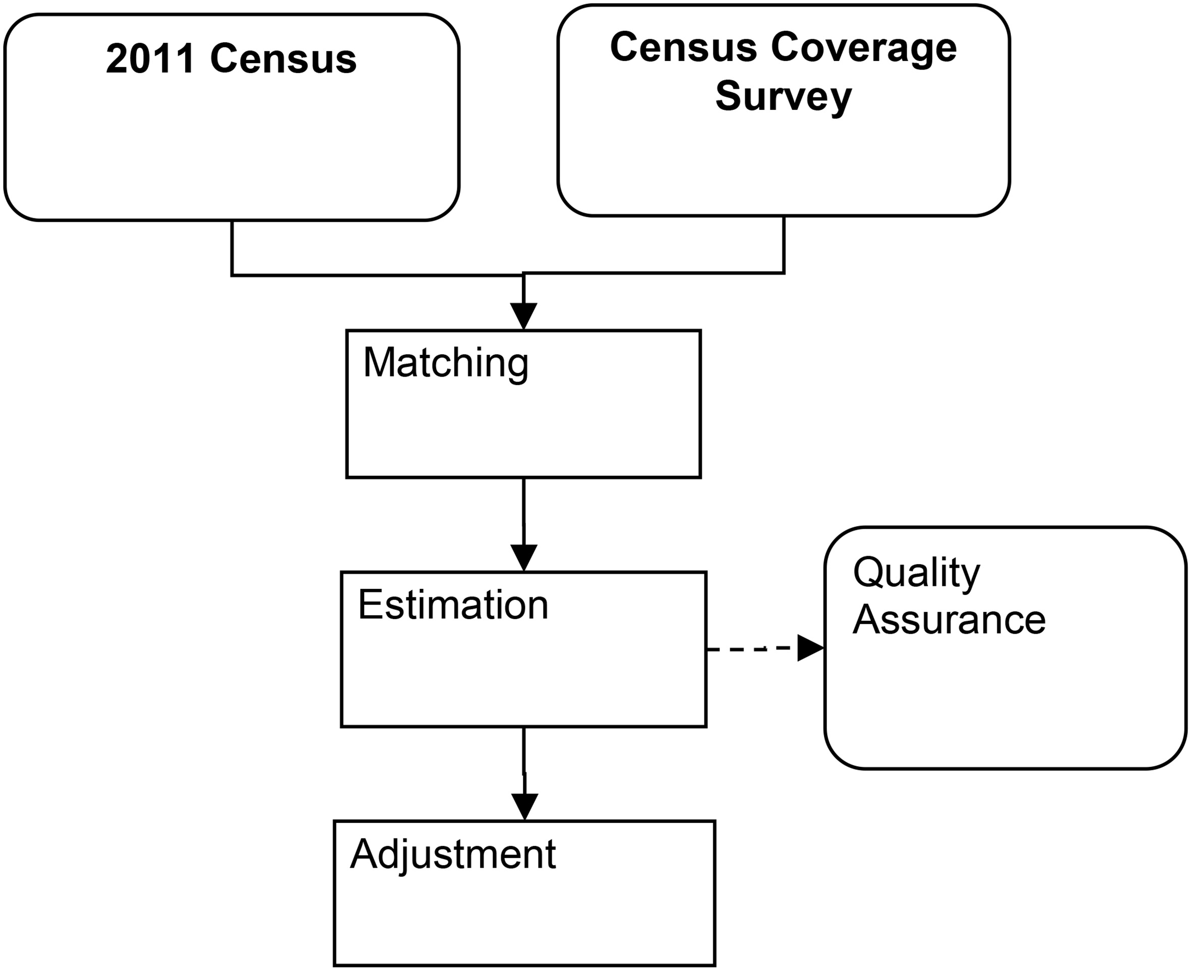
Evaluation of the one-number census approach used in the 2001 UK Censuses, see for example [22], broadly supported the strategy, and it was therefore adopted as the basis for coverage assessment and adjustment for the England and Wales census in 2011 (see [23]). The overall framework is shown in Fig. 1. The key source of data to combine with the census remained the CCS. The approach to the 2011 CCS design built on the structure used in 2001, but reflected the lessons learnt from the 2001 evaluations; it is discussed in [24].
Figure 1.
Overview of the 2011 coverage assessment and adjustment process.
In this paper we present the formal framework for the estimation of the household population by age-sex for a geographic region referred to as an estimation area (as outlined in Fig. 1), and evaluate the performance of the estimators under a variety of scenarios. The small area approach to estimation of the population size by age and sex within local authorities, the level at which local Government operates in the UK and therefore the key level for population size estimation, is discussed in [25] and the creation of the final database is outlined in [26]. We develop the approach to combine dual-system estimation with classic approaches to survey estimation in Section 2 and then test the performance of the estimator using simulations in Section 3. In Section 4 we cover several extensions including the development of a bootstrap approach to variance estimation and extending the dependence adjustments used in 2001 [5]. We finish with some discussion including issues relating to the actual implementation in 2011.
2.General estimation framework
The design of the CCS for 2011 is covered in detail in [24]. The structure of the survey essentially delivers an independent count of the population for a random sample of small areas. These areas are postcodes, collections of addresses used by the postal system, most with between 15 and 20 addresses. Postcodes are clustered together to form output areas (OAs), the lowest level of census output geography. OAs therefore formed the basis of the design, with sub-sampling of postcodes within selected OAs. The CCS was a stratified random sample of OAs, stratified using an index called the hard-to-count index [27] that classified OAs based on the predicted response rate in a census. Half of the postcodes (rounded up where necessary) within each OA were selected. In addition to the CCS sample of OAs, the census collected data for all the OAs. Therefore, the aim of the estimation framework was to combine the sampled data from the CCS with the census data from all areas to produce a better estimate of the population than given by the census alone.
2.1Ratio estimation
There is a long history of using a smaller-scale follow-up survey to improve estimates from a larger-scale data collection. [28] proposed sub-sampling the non-respondents from a relatively cheap mail survey covering a large sample, in our case that would be the census, and using an interview follow-up survey to obtain responses. This is essentially the field model for the actual census but with 100% follow-up. Another way is to think of the census as producing counts for all small areas but with error. This would be similar to the situation in business surveys where the frame has (imperfect) measures of employment and turnover based on historical administrative data for all units in the population. A business survey then measures the correct employment or turnover for a sample of units and this is used to correct the errors in the frame variables at some level of aggregation through ratio estimation. This concept sits behind the estimation framework for combining the CCS with the census. The follow-up survey to the census (in combination with the census) will allow us to estimate the correct counts but only for a sample of areas, and these can be combined with the census counts using ratio estimation. For ease of understanding we start by assuming the CCS obtains a perfect response for each sampled OA and then deal with the issue of non-response introducing errors into the CCS.
To formalise the estimation framework we start by specifying the structure of the sample. We have a sample of OAs
(1)
with the corresponding estimator of the total
(2)
[29] motivates this estimation strategy as the optimal approach within the class of linear estimators for the ratio model given in Eq. (2.1), as the estimator
This estimation structure fits exactly into the design structure and allows for variation in coverage across the age-sex groups within the design stratification defined by LA and local area using the HtC index. As the sampling design utilises a simple random sample of OAs within the design strata, an approximately design-unbiased ratio estimator, see [30], would have the same basic form for
(3)
and the estimated coverage ratio Eq. (2) becomes
(4)
The collapsing across the LAs produces unbiased estimates within a model-based framework, which are robust to departures from the variance assumption, provided that the expectation in the modified population model Eq. (2.1), a common ratio for LAs within an EA after controlling for age-sex and hard-to-count, holds for all LAs within the EA. When there are LA-specific differences in census coverage after controlling for the EA, the level of hard-to-count within the EA and the age-sex group, the common ratio assumption does not hold. Examples would be a localised failure of the Census Address Register or local problems with the census fieldwork to follow up non-responders.
When these LA specific effects exist, the modified population model Eq. (2.1) does not hold and then Eq. (4) is not unbiased with respect to the anticipated true population model Eq. (2.1) containing LA effects. A simple model-assisted estimator (see [31]) that reflects the sampling at the LA level, but estimates an overall ratio for the EA, adjusts Eq. (4) to give
(5)
where
From a purely model-based perspective it is hard to justify Eq. (5) as it is neither unbiased for the LA specific model Eq. (2.1), unless the sample is balanced within the strata used in Eq. (2.1) such that the sample mean of the
We can see from Eq. (5) that if the sampling fractions of OAs within a hard-to-count stratum for the LAs given by
The result is a general estimation strategy that utilises an estimator based on the separate ratio model Eq. (2.1) for all LAs with a sufficient sample to be a single LA estimation area, and an estimator based on the combined ratio model Eq. (2.1) for estimation areas formed by grouping LAs using an estimator of the coverage ratio defined by Eq. (4) as the default, but adjusted to Eq. (5) when the sampling fractions differ and there is evidence to support localised problems with census coverage. The enumeration ran satisfactorily in 2011, with no localised problems at the LA level, so the unweighted estimator Eq. (4) was utilised everywhere.
2.2Reflecting Census Coverage Survey (CCS) non-response
The framework outlined in Section 2.1 assumes that the CCS samples entire output areas (OAs) and perfectly re-enumerates them. In reality this is not true for two reasons. First, the final sampling units for the CCS are postcodes and these are clustered within OAs. The level of clustering is explored in [24] and some clustering of postcodes within OAs is seen as a good compromise between the statistical efficiency of an un-clustered design and the fieldwork advantages of some clustering. [24] proposed selecting three postcodes per OA but in the final design approximately half the postcodes within an OA were selected. On average, selecting three postcodes is equivalent to selecting half the postcodes from an OA but the number of postcodes per OA can vary considerably while the size of an OA does not by design vary unless there has been dramatic change on-the-ground since the 2001 Census. Second, the CCS did not achieve a 100% response from the usually resident population for census night any more than the original census did, and was expected to have slightly lower response than the census, because it was not compulsory. This was borne out in practice in 2011 with a CCS person response rate of 88.4% and a census response rate of 93.8%. Therefore, we first extend the framework to reflect sampling within postcodes and then deal with CCS non-response.
The population model Eq. (2.1) is extended to deal with sub-sampling of postcodes p within a sampled OA
(6)
where we still assume a common population ratio
(7)
where
We can define
(8)
However, we do not observe the true postcode counts
(9)
Therefore, we are defining
(10)
approximating the expectation of a ratio/product as the ratio/product of the expectations. Now applying the underlying probability structure of the dual-system model to each expectation in Eq. (2.2) we get
(11)
where
(12)
that applies the same approximation as in Eq. (2.2) but now conditioning on both the true population count
(13)
Therefore, the unbiased result in Eq. (2.2) still holds after the additional conditioning on the census count
(14)
Plugging in the result from Eq. (2.2) into Eq. (2.2) we now get
(15)
showing that the expectation in Eq. (2.2) still holds approximately when we replace the true postcode counts with their dual-system estimates; and any bias tends to zero as the postcode counts increase. Also, by applying the Chapman correction we can protect against the small sample bias of dual-system estimation, see Appendix for approximations of the equivalent results of Eqs (2.2) and (2.2).
We can also apply dual-system estimation at higher levels of aggregation. Using the cluster of postcodes rather than individual postcodes and following Eqs (2.2) and (2.2) we get
(16)
Remembering that the estimator for the coverage ratio Eq. (8) depends on the sum of the true postcode counts in the sample, we can now estimate that sum as
(17)
and applying the result Eq. (2.2) within the sum Eq. (17) we get
(18)
Therefore, applying the dual-system estimator at the cluster level does not impact on the approximate un-biasedness of the ratio model Eq. (2.2) and the estimator of the coverage ratio Eq. (8). However, we can see that in Eq. (2.2) we are now assuming the response probability for the CCS given by
Following the results in Eqs (2.2) to (18) we can move up to the level of the hard-to-count stratum
(19)
but we are now making the homogeneity assumption across the hard-to-count stratum
(20)
The approach outlined in [14, 6] is essentially Eq. (20) but includes the survey weights in the sample-based sums. These are important in the US context as their estimation strata, equivalent to our age-sex
Both the US approach [14, 15] and the approach outlined for the 2011 Census are based on both the Census and the CCS applying a usual residence rule as per Census Night. In Australia, the Census uses a person present base for enumeration while the coverage survey (PES) is based on usual residence for the production of official population estimates adjusted for census coverage errors. Therefore, the approach taken by the Australian Bureau of Statistics varies slightly but is still based on dual-system estimation as an estimate of the Census count based on the PES respondents is calibrated to the actual Census counts and this is then used to adjust the PES for non-response. This conceptually is like writing Eq. (20) as
(21)
where
2.3Summary of the estimation framework
The approach to estimation outlined in Sections 2.1 and 2.2 that combines ratio estimation with dual-system estimation at the level of the postcode or cluster of postcodes builds directly on the approach taken in 2001 [38, 5]. The difference between this approach and the application of dual-system estimation in the US, and to some extent Australia, is the use of low level geography in combination with age-sex groups to approximate the homogeneity assumption rather than a detailed cross-classification of characteristics within wide geographic areas. For 2011, the approach adopted also had the advantage of allowing sequential processing and estimation by geographic area rather than requiring all the data to be processed before estimation could commence. However, prior to 2011, there was a decision to make regarding the ultimate level of clustering for the dual-system estimator as well as whether to implement ratio estimation as outlined above or the more complex approach from 2001. The 2001 approach [38] used the cluster of postcodes but then implemented a robust approach to the out-of-sample predictions requiring the cluster to be broken-down into the constituent postcodes. The next section will explore these issues using a simulation study built on the extensive data available from 2001.
3.Simulation study
For the 2001 Census, extensive simulations were used to evaluate the approach to estimation and coverage adjustment [3, 38, 4, 5]. These used coverage probabilities developed in [38] that were based on the limited knowledge of census coverage in 1991 to simulate censuses and CCSs. However, when developing the 2011 methods, it was possible to use the actual patterns found in 2001 for both the census and the CCS to define detailed coverage probabilities for both households and individuals. In this section we outline the simulation approach used for 2011 and its use in testing the estimation approach outlined in Section 2.
3.1Design of the simulation study
A series of multilevel logistic regression models [39] were fitted at the national (England and Wales) level to the linked 2001 Census and CCS data. The model levels reflected the geographical hierarchy of the census with LAs and then OAs. Four logistic models were fitted using the matched data; one for coverage of households in the census as measured by the CCS responses, one for coverage of individuals in the census as measured by the CCS responses, one for coverage of households in the CCS as measured by the census responses, one for coverage of individuals in the CCS as measured by the census responses. The characteristics used in the models are given in Table 1. In general the patterns observed for the variables were as expected; lower coverage of private rented households, lower coverage of young adults and particularly young men, lower coverage for higher levels of the hard-to-count index (captured by a continuous hard-to-count score). Also, CCS coverage tends to vary less than census coverage, apart from household size, which is more important for the household coverage in the CCS than for household coverage in the census. This is likely due to it being an interview rather than self-completion of a questionnaire delivered by an enumerator, with contact being more difficult for smaller households. Full details of the models can be found in [40].
Table 1
Description of the variables included in the four models for census and CCS by individual and household coverage
| Variables included in the models for coverage at the individual level | |
|---|---|
| Variable name | Categories |
| Age-sex | Babies, Males 1 to 4, Males 5 to 9, Males 10 to 14, Males 15 to 19, …, Males 85 |
| Marital status | Single, Married, Remarried, Separated, Divorced, Widowed |
| Primary activity last week | Working full-time/part-time or temporarily sick, Looking for work, Waiting to start work, Full time education, Permanently sick or disabled, Retired, Looking after home/family or none, Under 16/over 75 |
| Variables included in the models for coverage at both the individual and household level | |
| Household tenure | Owns outright, Owns with mortgage, Part rent/part mortgage, Rents from council, Rents from housing association, Rents from private landlord, Other |
| Household ethnicity | All any white, All any black/black British, All any Asian, All Chinese or other, Any other combination |
| Household structure | Single male 15–34, Single female 15–34, Single person 80 |
| Household size | Continuous with linear and quadratic terms |
| Hard-to-count score for OA | Continuous with linear and quadratic terms |
| Government office region | North East, North West, Yorkshire and the Humber, East Midlands, West Midlands, East of England, London (Outer), London (Inner), South East, South West, Wales |
Table 2
Performance estimating the population total using ratio estimation combined with DSEs at various levels
| Overall relative bias (%) | Overall RRMSE (%) | Overall RSE (%) | ||||||||||
|---|---|---|---|---|---|---|---|---|---|---|---|---|
| Estimation area | Estimation area | Estimation area | ||||||||||
| DSE level | LJ | NX | KO | NA | LJ | NX | KO | NA | LJ | NX | KO | NA |
| Perfect CCS | 0.28 | 0.14 | 0.07 | 0.20 | 1.43 | 1.37 | 0.89 | 0.84 | 1.40 | 1.36 | 0.89 | 0.82 |
| Postcode | 0.00 | 1.48 | 1.56 | 0.88 | 0.78 | 1.36 | 1.32 | 0.87 | 0.78 | |||
| Cluster |
|
|
| 0.08 | 1.44 | 1.41 | 0.90 | 0.80 | 1.43 | 1.38 | 0.90 | 0.79 |
| Hard to count |
|
|
| 0.10 | 1.43 | 1.40 | 0.89 | 0.81 | 1.43 | 1.39 | 0.89 | 0.80 |
| 2001 robust ratio | 0.43 | 1.35 | 1.43 | 0.83 | 0.94 | 1.28 | 1.29 | 0.81 | 0.84 | |||
| Simulated census | ||||||||||||
| 2001 Undercount | ||||||||||||
The models were used to predict a household coverage probability and an individual coverage probability for every responding household and individual in the 2001 Census database for both the census and the CCS. The estimated LA random effects were used directly within each LA to represent residual variation in coverage at the LA level. At the OA level, only a sample of OAs had an observed random effect based on the 2001 CCS sample. Therefore, sampling with replacement from the estimated OA random effects within region by hard-to-count classes was used to assign a random effect to all OAs that would represent reasonable residual variation at the OA level. This was done so that all four estimated random effects from a single sampled OA provided the random effects for an OA in the full database to preserve any relationships between the random effects at an OA level. Within the simulation, the household probabilities were used to simulate whether a household was covered in either the census or CCS. As a default this was decided independently for the two outcomes. Then, if a household was simulated as being counted in either the census or CCS, within household coverage of individuals was simulated using a conditional probability defined by the individual’s overall coverage probability divided by their household coverage probability with a maximum of one. Finally, households were removed if all the individuals over 15 were missed at the within household stage to avoid coverage of households without any adults.
Four hundred simulations were undertaken across the country. Each iteration simulated the coverage of individuals and households for the whole database and selected the CCS sample for that iteration. The design of the CCS was a simplified version of the 2011 design based on stratifying by LA, then by hard-to-count index within each LA, and then selecting a simple random sample of OAs in each stratum. Finally, three postcodes per OA were selected. The choice of OA and postcode for the structure are discussed in more detail in [24]. For this evaluation the allocation of OAs was proportional to the number of OAs meaning that at estimation, sample design effects do not interfere with using model Eq. (2.1) and coverage estimator Eq. (4) when dealing with an estimation area based on several LAs.
3.2Simulation results
Summary results at the level of the total population are presented in Table 2 for a set of four EAs that cover a range of coverage scenarios as well as being a combination of a single LA per EA and multiple LAs per EA. The EA coded LJ covers a set of LAs in London and was a lower coverage area in 2001. The EA coded NX is a single LA area and covers a large metropolitan city. This is included both as an example of a single LA area and also because such cities were problematic for the 2001 Census coverage assessment [41]. The EA coded KO has two urban LAs and had an average level of coverage in 2001. Finally, the EA coded NA has multiple LAs mixing urban and rural populations with a higher 2001 coverage. The four EAs combined cover a population of 1.98 million with simulated census coverage of around 90.8%, which is lower than was anticipated for the national population in 2011.
The simulation results in Table 2 cover a variety of scenarios including a perfect CCS (model Eq. (2.1) with Eq. (4) as the coverage ratio) and adjustments for survey non-response using the dual-system estimator (DSE) at the level of the postcode, cluster of postcodes, and at the hard-to-count level. Results are also presented for the robust ratio approach implemented in 2001 (see [38] for full details) that reduced the influence of outliers when making out-of-sample predictions. Performance is assessed in terms of the empirical relative bias, empirical relative root mean square error (RRMSE), and empirical relative standard error (RSE) as estimated by the 400 iterations of the simulation. The empirical bias for the simulated census is also presented and compared to the estimated census bias for each EA in 2001. In general, the empirical bias for the simulated census tracks the estimated 2001 coverage. The noticeable exception is for estimation area NX, which is the large metropolitan city, where the simulated census coverage, based on the modelling of the 2001 CCS data from the whole country, is lower than the estimated coverage for 2001. The difference makes sense in this case as additional adjustments were made to the population estimate of NX post-2001 due to concerns about the performance of the CCS sample in that specific estimation area, implying that census coverage in 2001 was worse than the original estimate reported in Table 2.
The results in Table 2 for the perfect CCS give a benchmark to compare to as well as demonstrating the technical bias of ratio estimation under repeated sampling. The first term in this bias [30, p. 161] has the form
where
As CCS non-response is allowed for, Table 2 confirms previous work for 2001 [38] that at the postcode level the DSE tends to under-estimate, even with the Chapman correction. This ties in with the discussion of the properties of the Chapman correction [33] when the condition
The 2001 robust ratio approach also performs generally as expected; it induces a negative bias but reduces the RSE so that the overall RRMSE is not compromised. However, these more detailed simulations than were possible prior to 2001 suggest that the simple ratio is not as sensitive to extreme estimates; and the simpler approach has the attraction of being more transparent to users while not inducing negative bias. There was also less concern coming in to 2011 regarding extreme over-estimates as there was more confidence in the quality assurance process and its ability to detect a gross error, positive as well as negative. Figure 2 provides further evidence to support simple ratio estimation rather than the robust approach showing performance for males by age-group comparing to a perfect CCS across the four EAs. For the estimation area NX, Fig. 3 demonstrates how the robust approach reduces the impact of the extreme errors for both males and females, but this reduction is not as visually obvious as in the simulation results in [38] undertaken prior to 2001.
Figure 2.
Relative bias and RRMSE for males by age group for a perfect CCS, and DSE applied at cluster level with both simple ratio estimation and the 2001 robust ratio method.
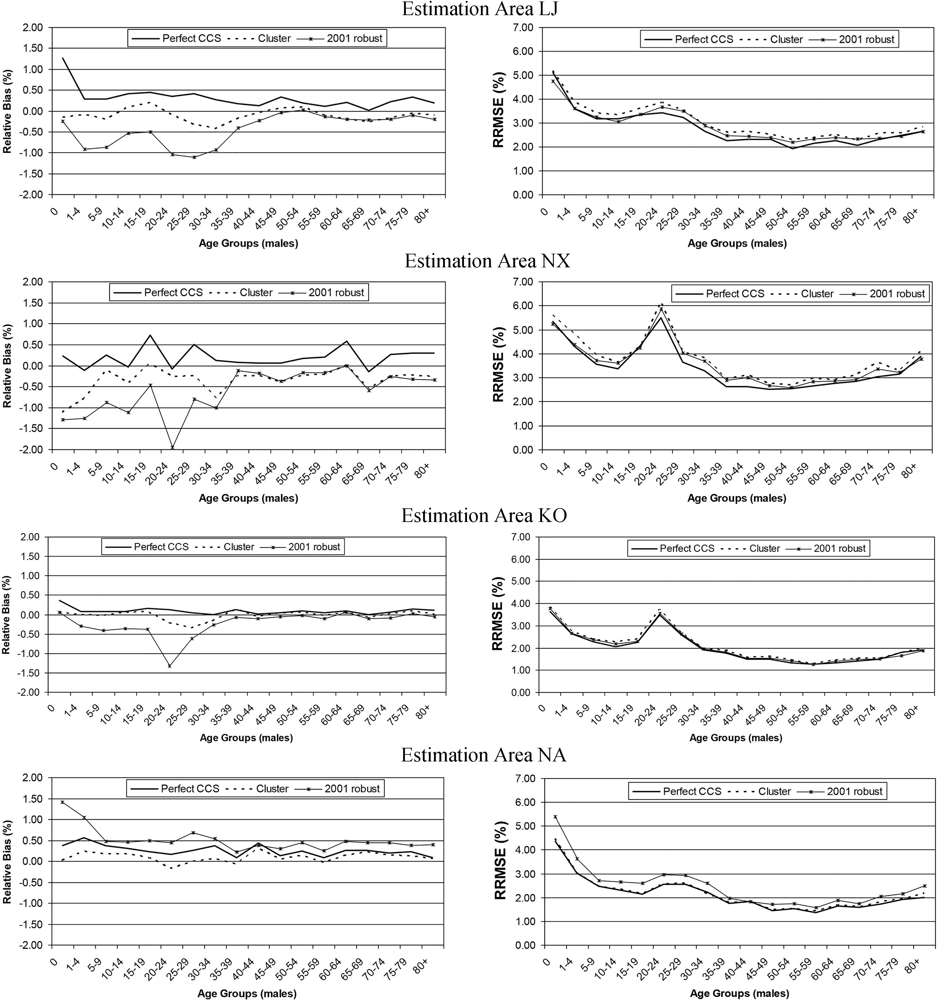
Figure 3.
Relative error distributions by age and sex for estimation area NX with the cluster level DSE.
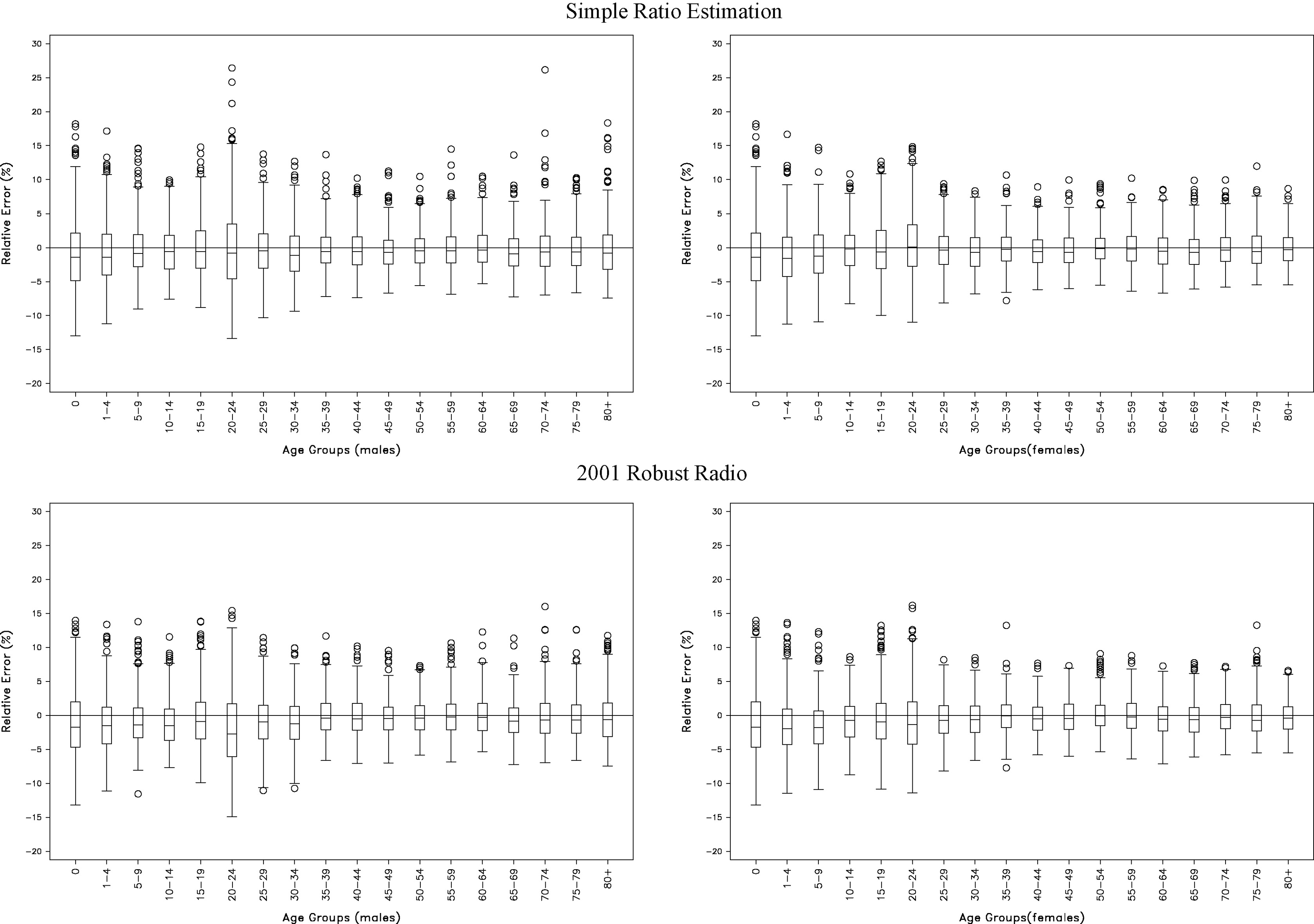
Figure 4.
Mean sex ratios for simple ratio estimation with the cluster level DSE and the census compared to the truth.
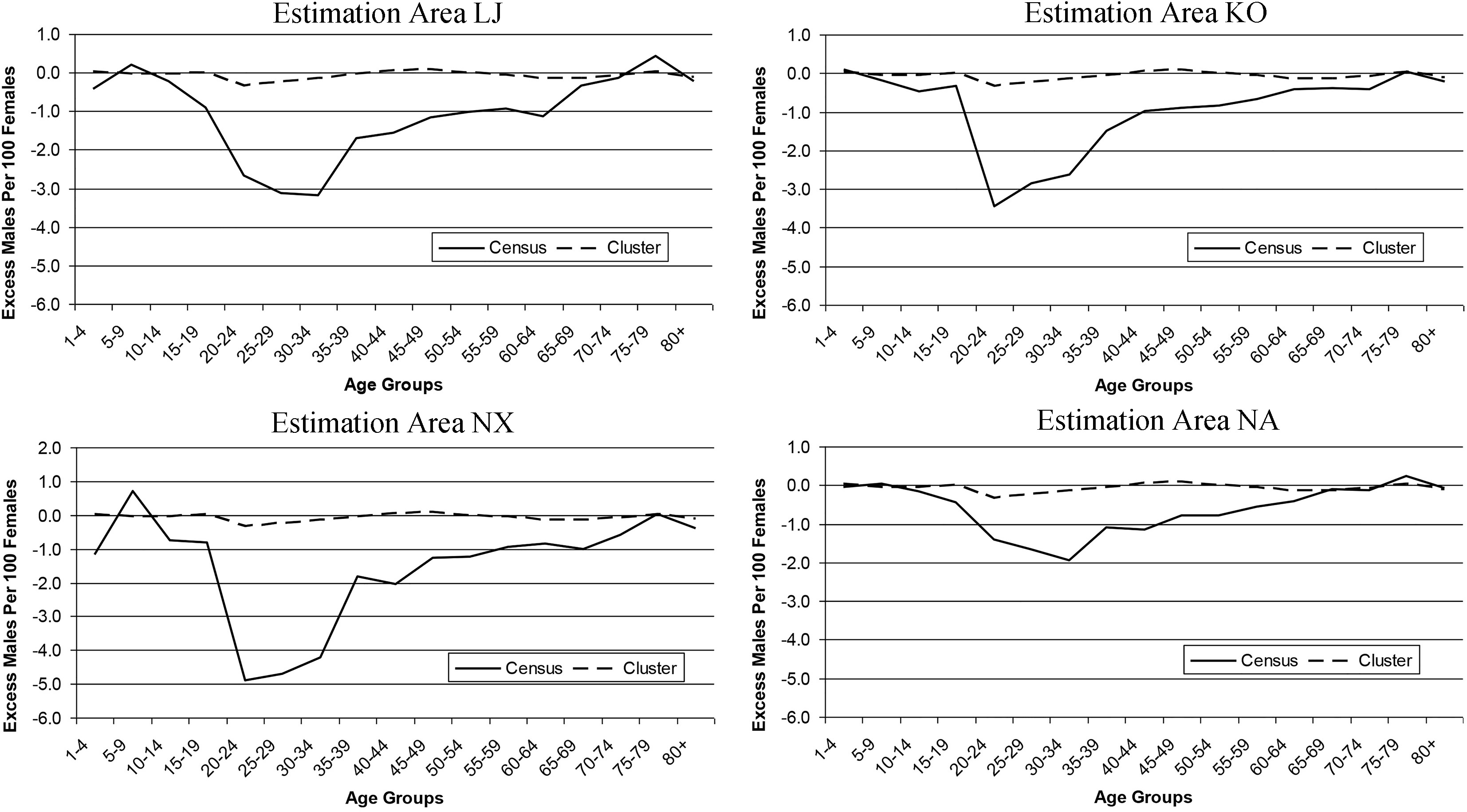
Taking the results of Table 2 with Figs 2 and 3, the findings supported adopting an estimation strategy using cluster level DSE with simple ratio estimation as developed in Section 2 for the 2011 Census. Figure 4 shows the average error in the sex ratio for the simulated census enumeration compared with the error for this estimation strategy across age groups for the four EAs. This adds to the results for males in Fig. 2 to demonstrate that estimation with the CCS not only reduces the bias in the age-sex estimates but also corrects for the differential nature of the bias in the census leading to a more plausible sex ratio. Therefore, pulling together the simulation results with the other issues discussed earlier led to the adoption of cluster level DSE with simple ratio estimation to produce the age-sex population estimates at the EA level for the 2011 Census in England and Wales. Based on this work the same basic strategy was also implemented for Scotland and Northern Ireland within their EA and hard-to-count structures.
4.Extending the estimation strategy
The simulation results in Section 3 demonstrate that the framework for estimation proposed in Section 2, building on the 2001 approach [38], has good properties with respect to both bias and variability when combining cluster level dual-system estimation, Eqs (2.2)–(18), with simple ratio estimation. However, to implement the framework for the 2011 Census, several additional issues needed to be dealt with. In this section we consider variance estimation, adjusting for dependence, adjusting for over-count, the issue of movers and the practical issue of collapsing age-sex categories when estimating in specific estimation areas.
4.1Variance estimation
For the 2001 Census estimates, a jackknife approach was developed to produce variance estimates for the main age-sex outputs [38]. While this approach performed well under simulation, it was difficult to reflect fully all the sources of variation, such as the dependence adjustments that were made to the final estimates, although simulations suggested that any increase in variability was marginal [5]. The alternative bootstrap approach [42] was not explored for 2001 but advances in computing, as well as more practical applications of bootstrapping in finite population sampling [43], made this an attractive proposition for 2011. The work on bootstrapping also explored the practical application of asymmetric empirical confidence intervals with bias corrections [44] as this is attractive in the context of estimating the population total based on a coverage ratio that is intrinsically greater than one, especially when the ratio gets close to one.
Table 3
Estimates of the variance of the population total estimator with corresponding coverage for 95% confidence intervals
| Bootstrap | ||||||
|---|---|---|---|---|---|---|
| Simulation | Jack knife | z-interval | t-interval | BC interval | BCA interval | |
| Variance | 19,683,414 | 21,418,196 | 19,468,872 | |||
| Coverage of 95% CI | – | 93.00 | 91.75 | 92.25 | 92.50 | 91.75 |
Figures extracted from [45], Tables 1 and 2.
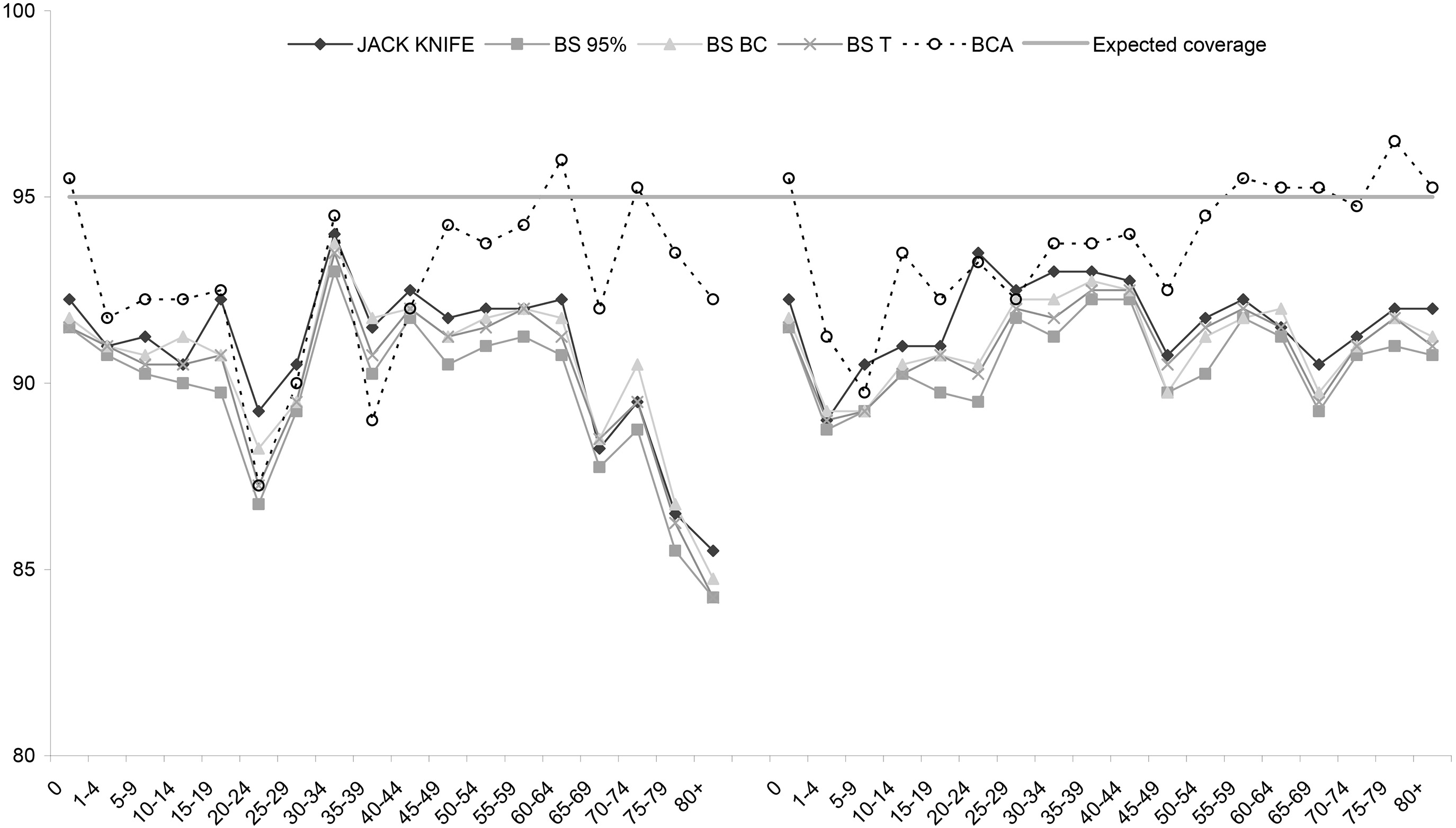
Results presented in [45] were based on the same simulations as used in Section 3, with the addition of 2000 replicates when implementing the bootstrap methods. Table 3 reproduces the performance for estimating total population for KO, one of the EAs used in Section 3. In terms of estimating the variance, the average of the bootstrap estimates is close to the empirical variance given by the simulation, while the jack-knife approach is a little conservative. Note that a variance of around 20 million for the total population corresponds to a standard error of less than 5,000 and an RSE of less than one per cent. In terms of confidence interval coverage, all the approaches give slight under-coverage. As might be expected, using a
Figure 5.
Coverage of 95% confidence intervals by age sex group for estimation area KO.
The development work suggested that a bootstrap approach was plausible and the independent review of the 2011 methodology by [46] supported both the use of bootstrap and the development of asymmetric empirical confidence intervals. Adopting the approach also gave flexibility to estimate confidence intervals for the population estimates of those LAs produced using small area approaches [25]; and bootstrap methods are now common when estimating variances [47] for estimates produced using small area methods [48].
4.2Adjusting for dependence
Key to the application of DSE is independence between the counts for the two sources. This is evident in Eq. (2.2), where the joint probability of coverage is the product of the two marginal probabilities; while in Eq. (2.2) it is the assumption that the CCS coverage for those counted in the census is equal to the overall coverage of the CCS. The independence assumption is likely to fail for one of three reasons: a lack of operational independence between the census and CCS; an individual or household’s conditional response to the CCS depending directly on their known response status in the census; or apparent dependence due to a failure of the homogeneity assumption of the DSE.
The first is tackled by ensuring CCS operations, staffing and fieldwork period are independent of the census; and in 2011 this was further strengthened as the data collection approach for the CCS, with a field-listing of households followed by door-step interviews, was quite different to the census using a post-out, post-back approach with follow-up, based on an address register. The second is minimised by ensuring the CCS interviewers do not focus on the CCS as a check on the census enumeration for the household, but rather an independent check on the performance of ONS. Any reverse dependence, referring to a household being prompted to post-back a census form after completing the CCS interview, was also removed, as late returns for the census were not allowed into the data used for DSE and ratio estimation.
Table 4
Odds ratios applied to simulations to induce dependence
| Estimation area | Odds ratios applied to simulations by | Simulation census coverage (%) | ||
|---|---|---|---|---|
| hard-to-count level | ||||
| Easy | Medium | Hard | ||
| LJ (Outer London area) | 2.2 (18) | 3.8 (41) | 3.3 (41) | 86.7 |
| NX (North-West area) | 1.0 (13) | 4.4 (48) | 1.5 (39) | 87.8 |
| KO (Midlands area) | 1.0 (44) | 5.6 (43) | 4.4 (13) | 93.9 |
| NA (North-West area) | 2.2 (59) | 1.0 (33) | 1.0 (8) | 95.2 |
Table 5
Performance estimating the population total using ratio estimation combined with DSEs for different scenarios relating to dependence
| Overall relative bias (%) | Overall RRMSE (%) | Overall RSE (%) | ||||||||||
|---|---|---|---|---|---|---|---|---|---|---|---|---|
| Estimation area | Estimation area | Estimation area | ||||||||||
| CCS scenarios | LJ | NX | KO | NA | LJ | NX | KO | NA | LJ | NX | KO | NA |
| Perfect CCS | 0.28 | 0.14 | 0.07 | 0.20 | 1.43 | 1.37 | 0.89 | 0.84 | 1.40 | 1.36 | 0.89 | 0.82 |
| Independence | 0.08 | 1.44 | 1.41 | 0.90 | 0.80 | 1.43 | 1.38 | 0.90 | 0.79 | |||
| Unadjusted | 2.48 | 2.00 | 1.02 | 0.78 | 1.25 | 1.33 | 0.84 | 0.78 | ||||
| 2001 adjustment | 0.11 | 1.56 | 1.53 | 0.93 | 0.81 | 1.43 | 1.45 | 0.92 | 0.80 | |||
| Revised approach | 0.11 | 1.47 | 1.48 | 0.90 | 0.80 | 1.47 | 1.47 | 0.90 | 0.80 | |||
Despite these efforts, and the use of localised DSEs in estimation to approximate homogeneity, there is always the risk of some residual dependence (actual or apparent). An approach using national sex ratios, with the assumption of a correct female count, was proposed by [49]. This was applied by the US Census Bureau to assess the sensitivity of the 1990 Census results [50]; and extended to a Bayesian framework in [51]. It also features in the evaluation of the 2010 Census [16]. In England and Wales post 2001, a dependence adjustment was made and reflected in the published estimates. The approach was developed and implemented in [5] and differs from the US Census Bureau approach of using national sex ratios. Instead it relied on an alternative count of the number of households for a region and consequently made specific adjustments within each region.
For 2011 we developed the 2001 approach to build on its successful implementation while also taking advantage of additional information available in 2011. In particular, we assumed the use of post-out for the actual 2011 Census would strengthen estimation of an alternative household count based on the postal system at the level of each EA, allowing the odds ratios to vary across EAs within the same region. We also explored direct estimation (for each EA within broad age-sex groups) of the parameters
To test the ideas the simulation approach of Section 3 was extended to allow for dependence at the household level, similar to the simulation approach in [5]. The odds ratios used in each EA by HtC came from the estimated odds ratios for the appropriate regions in 2001 to ensure they were plausible and are shown in Table 4, along with the distribution of OAs by HtC within each EA. Therefore, the main comparisons are within an EA where other features remain constant, rather than between EAs; although between EAs we can get a sense of performance for differing scenarios. Table 5 then gives the performance of different estimation strategies for the total population. The perfect CCS and independence scenarios with cluster level DSE are also shown as benchmarks. Once dependence is introduced the unadjusted scenario shows the potential bias in the estimates; particularly when lower census coverage is combined with higher levels of dependence as demonstrated by LJ and NX. This confirms the results presented in [5] where the simulation study has a more extensive set of scenarios for the odds ratios. The 2001 adjustment uses the same fixed parameters as were used in the actual 2001 approach, and as observed in [5] reduces the bias relative to no adjustment for only a small increase in the RSE relative to the DSE under independence. The revised approach refines this adjustment to directly estimate the parameters
4.3Adjusting for over-count
In 2001, with a traditional census delivery and follow-up after post-back, it was expected that over-count would be a very minor issue relative to under-count; and therefore the estimation from the CCS for over-count was more of a quality measure than part of the main estimation. The level estimated by the CCS was around 0.1% and subsequent work by ONS suggested it may have been closer to 0.4% (as reported in [52]). However, with the 2011 Census moving to a post-out model similar to that used in the US it was recognised that over-count was potentially a larger consideration than in 2001 and needed to be directly adjusted for in the coverage estimation. The US-based E-sample approach, as outlined in [6], was rejected as additional fieldwork would require too much additional resource. Therefore, it was not possible to directly adjust the
Using an extension to the simulations presented in Section 3, [52] demonstrated that the approach was effective at removing bias due to over-count, and like the dependence adjustments in Section 4.2, had only a small impact on the RSEs of population estimates. The bootstrap approach to variance estimation also offered the flexibility to reflect this increase in variability in the estimated RSEs.
4.4Issue of movers
One of the assumptions behind DSE is that both the census and survey are measuring the same (closed) population. However, in reality, the CCS took place a short period after Census Day so the household population could change due to ‘births’ or ‘deaths’. Births created by literal births, or individuals joining a household, are dealt with as the CCS explicitly collected data relating to the usually resident population on Census Day. Likewise, ‘deaths’ can be identified provided at least one member of the Census Day household remained to respond to the CCS. However, moves by complete households essentially created ‘deaths’ in the area where they were on Census Day and ‘births’ in the new area for the CCS. Using the analysis of movers undertaken by the US Census Bureau in [53], which treats movers as a source of heterogeneity bias and therefore apparent dependence, leads to a bias given by
(22)
where
Assuming
The aim was not to use Eq. (22) directly to adjust for heterogeneity bias caused by movers, but as a quality check on the household level dependence adjustments outlined in Section 4.2. As it was only whole households moving that caused an issue, the impact would be an apparent dependence at the household level; and that is exactly the level at which the dependence adjustment framework was targeted.
4.5Collapsing categories
An additional issue that required consideration for full-scale implementation was the treatment of age-sex categories when the sample numbers were small. Where the census or CCS sample counts were small in any age-sex group cell, this could result in unstable estimates. This can be a particular problem when working with some of the older age-sex groups and specially defined age-sex groups, which do not follow the standard five year pattern, to deal with the change from schooling to work or student status over the range 16 to 19, as well as the high under-count for babies. ONS implemented a strategy to deal with this issue by collapsing age-groups in different dimensions to ensure sufficient sample counts in each cell, reduce the variance of estimates, and therefore reduce the relative width of confidence intervals; while reflecting expected differences in coverage patterns by age, sex, and HtC.
Age-sex categories were collapsed to deal with inconsistencies in the estimated coverage rates by HtC, specifically when they did not follow the pattern of increasing estimated coverage rates for more difficult HtC groups – for example: a low, medium and high pattern for estimated coverage rates in HtC 3, 2 and 1 respectively. In some cases, a large differential in estimated coverage rates between adjacent age groups was plausible. Where this was not the case, the age-sex groups were collapsed. For example, large differences were observed between student populations and an adjacent age group such as male 25 to 29 year-olds, but it was less plausible to observe a large difference between the male 40 to 44 and male 45 to 49 age groups.
Occasionally, it was necessary to correct implausible sex ratio patterns by collapsing age-sex groups to smooth the sex ratio. Collapsing across sex was recommended for young age groups because coverage rates should be more similar across sex, rather than across age groups. In other words the expectation was that coverage for male and female 0–2s would be similar – there was no reason why one gender was missed more than the other at these ages. Additionally, collapsing student age groups (18 year-olds, 19 to 24 year-olds) with younger age groups (8 to 17 year-olds) was avoided wherever possible, usually by collapsing 18 year-olds with 19 to 24 year-olds, or by collapsing across sexes.
5.Discussion
This paper covers the development of the estimation strategy that was used to produce the key age-sex estimates following the 2011 Census of England and Wales. The approach built on the 2001 estimation strategy but refinements were made based on the more extensive simulation work that was possible. The estimation strategy was also developed to fit with the revised design for the 2011 Census Coverage Survey [24]. The simulations presented here demonstrate the appropriateness of the general estimation framework as well as the performance of developments to reflect adjustments for dependence and the approach to variance estimation. This, along with the work to develop over-count adjustments created the information that led to the framework being the basis of the 2011 estimation strategy following an endorsement by the independent review [46].
Subsequent to the implementation of the estimation framework following the 2011 Census, the quality assurance process reported in the evaluation report [54] shows it performed well to produce the basic population estimates. A small additional dependence adjustment was made at the national level using an agreed sex ratio based on administrative sources external to the census process. This was likely due to residual within household dependence amongst young adult males that would not have been removed by the dependence adjustment based on a household count. The report also explains some additional adjustments that were made to the ratio estimation framework when administrative data suggested the CCS sample was not well distributed within an estimation area.
Looking forward to the 2021 Census and beyond, further developments can be made to more closely integrate administrative data. Linkage at the unit record level, even for a small sub-sample, presents opportunities to further enhance the dependence adjustments as three sources allow for the direct estimation of the dependence relationship between the census and the coverage survey. As mentioned, the final implementation of the estimation framework [54] included as an addition the potential to adjust the estimates if administrative data suggested the CCS sample was poorly distributed. Going forward, this should be more fully integrated into the estimation framework, as over-count and dependence adjustments were in 2011, and greater use of administrative data at the design stage of the CCS would also help to ensure the sample is distributed as effectively as possible. Finally, although the bootstrap approach was successfully implemented for the 2011 estimates, the confidence intervals were not based on the empirical distribution. Further work is needed to explore the use of empirical confidence intervals as originally planned for 2011.
Acknowledgments
The authors thank the members of the various census committees that have commented on this work as it has developed. They would specifically like to acknowledge the contribution and support of Dr Frank Nolan from ONS, who passed away unexpectedly in 2012, in the development of the coverage assessment plans for the 2011 Census.
References
[1] | OPCS. Rebasing the annual population estimates. Population Trends (1993) ; 73: : 22-5. |
[2] | Heady P, Smith S, Avery V. 1991 Census Validation Survey: Coverage Report. London: Her Majesty’s Stationery Office; (1994) . |
[3] | Brown JJ, Diamond ID, Chambers RL, Buckner LJ, Teague AD. A methodological strategy for a one-number census in the UK. Journal of the Royal Statistical Society Series A (1999) ; 162: : 247-267. |
[4] | Steele F, Brown J, Chambers R. A controlled donor imputation system for a one-number census. Journal of the Royal Statistical Society, Series A (2002) ; 165: : 495-522. |
[5] | Brown J, Abbott O, Diamond I. Dependence in the 2001 one-number census project. Journal of the Royal Statistical Society Series A (2006) ; 169: : 883-902. |
[6] | United Nations. Post Enumeration Surveys; Operational guidelines. New York: United Nations; 2010 [cited (2017) Oct 1]. Available from: http://unstats.un.org/unsd/demographic/standmeth/handbooks/Manual_PESen.pdf. |
[7] | Isaki CT, Ikeda MM, Tsay JH, Fuller WA. An estimation file that incorporates auxiliary information. Journal of Official Statistics (2000) ; 16: : 155-172. |
[8] | Marks ES, Parker Mauldin W, Nisselson H. The post-enumeration survey of the 1950 census: a case history in survey design. Journal of the American Statistical Association (1953) ; 48: : 220-243. |
[9] | Coale AJ. The population of the United States in 1950 classified by age, sex, and color – a revision of census figures. Journal of the American Statistical Association (1955) ; 50: : 16-54. |
[10] | Bailar BA, Jones CD. The evaluation of the 1980 decennial census. The Statistician (1980) ; 29: : 223-235. |
[11] | Wolter KM. Some coverage error models for census data. Journal of the American Statistical Association (1986) ; 81: : 338-346. |
[12] | Sekar CC, Deming WE. On a method of estimating birth and death rates and the extent of registration. Journal of the American Statistical Association (1949) ; 44: : 101-115. |
[13] | Hogan H. The 1990 post-enumeration survey: an overview. The American Statistician (1992) ; 46: : 261-269. |
[14] | Hogan H. The 1990 post-enumeration survey: operations and results. Journal of the American Statistical Association (1993) ; 88: : 1047-1060. |
[15] | Hogan H. The accuracy and coverage evaluation: theory and design. Survey Methodology (2003) ; 29: : 129-138. |
[16] | US Census Bureau. 2010 Census Coverage Measurement (CCM) Workshop, January 12–13, 2009, Washington, D.C. Washington: US Census Bureau; 2009 [updated 2015 Aug 21; cited (2017) Oct 1]. Available from https://www.census.gov/coverage_measurement/post-enumeration_surveys/2010_ccm_workshop.html. |
[17] | Bell P, Clarke C, Whiting J. An estimating equation approach to census coverage adjustment. ABS Research Paper 1351.0.55.019; (2007) . |
[18] | Chipperfield J, Brown J, Bell P. Estimating the count error in the Australian census. Journal of Official Statistics (2017) ; 33: : 43-59. |
[19] | Renaud A. Estimation of the coverage of the 2000 census of population in Switzerland: Methods and results. Survey Methodology (2007) ; 33: : 199-210. |
[20] | Kamen CS. The 2008 Israel integrated census of population and housing. Statistical Journal of the United Nations ECE (2005) ; 22: : 39-57. |
[21] | Belley C, Clark C, Ha B, Switzer K, Tourigny J. Coverage: 1996 census technical reports. Ottawa: Statistics Canada; (1999) . Catalogue No. 92-370-XIE. |
[22] | Office for National Statistics. Census 2001 review and evaluation: One Number Census evaluation report. London: Office for National Statistics; 2005 [cited (2017) Oct 1]. Available from http://www.ons.gov.uk/ons/guide-method/census/census-2001/design-and-conduct/review-and-evaluation/evaluation-reports/one-number-census/evaluation-report.pdf. |
[23] | Abbott O. 2011 UK Census Coverage assessment and adjustment strategy. Population Trends (2007) ; 127: : 7-14. |
[24] | Brown J, Abbott O, Smith PA. Design of the 2001 and 2011 census coverage surveys for England and Wales. Journal of the Royal Statistical Society Series A (2011) ; 174: : 881-906. |
[25] | Baffour B, Silva D, Veiga A, Sexton C, Brown J. Small area estimation strategy for the 2011 Census in England and Wales. Statistical Journal of the International Association for Official Statistics (2018) ; 34: : 395-407. |
[26] | Brown J, Sexton C, Taylor A, Abbott O. Coverage adjustment methodology for the 2011 Census. Titchfield: Office for National Statistics; 2011 [cited (2017) Oct 1]. Available from http://www.ons.gov.uk/ons/guide-method/census/2011/the-2011-census/processing-the-information/statistical-methodology/coverage-adjustment-methodology-for-the-2011-census.pdf. |
[27] | Abbott O, Compton G. Counting and estimating hard-to-survey populations in the 2011 Census. In: Tourangeau R, Edwards B, Johnson TP, Wolter KM, Bates NA, eds. Hard-to-Survey Populations. Cambridge: Cambridge University Press; (2014) . |
[28] | Hansen MH, Hurwitz WN. The problem of non-response in sample surveys. Journal of the American Statistical Association (1946) ; 41: : 517-529. |
[29] | Royall RM. On finite population sampling under certain linear regression models. Biometrika (1970) ; 57: : 377-387. |
[30] | Cochran WG. Sampling techniques, 3 |
[31] | Särndal C-E, Swensson B, Wretman J. Model Assisted Survey Sampling. New York: Springer-Verlag; (1992) . |
[32] | Scott AJ, Holt D. The effect of two-stage sampling on ordinary least squares methods. Journal of the American Statistical Association (1982) ; 77: : 848-854. |
[33] | Seber GAF. The estimation of animal abundance and related parameters, 2 |
[34] | Chao A, Tsay P, Lin S, Shau W, Chao D. The applications of capture-recapture models to epidemiological data. Statistics in Medicine (2001) ; 20: : 3123-3157. |
[35] | Van der Heijden PGM, Whittaker J, Cruyff M, Bakker B, Van der Vliet R. People born in the middle east but residing in the Netherlands: Invariant population size estimates and the role of active and passive covariates. The Annals of Applied Statistics (2012) : 6: : 831-852. |
[36] | Chapman DG. Some properties of the hypergeometric distribution with applications to zoological censuses. University of California Publications Statistics (1951) ; 1: : 131-160. |
[37] | Martin D. Geography for the 2001 Census in England and Wales. Population Trends (2002) ; 108: : 7-15. |
[38] | Brown JJ. Design of a census coverage survey and its use in the estimation and adjustment of census underenumeration. PhD Thesis. Southampton: University of Southampton; (2000) . |
[39] | Goldstein H. Multilevel Statistical Models, 4th edn. Chichester: Wiley; (2011) . |
[40] | Brown J, Sexton C. Estimates from the census and census coverage survey. GSS Methodology Conference, London, June 2009. ONS; 2009 [cited (2017) Dec 18]. Available from https://www.ons.gov.uk/ons/media-centre/events/past-events/conference/population-estimates-from-the-census-and-census-coverage-survey-paper.pdf. |
[41] | Office for National Statistics. 2001 Census: Manchester and Westminster matching studies full report. London: Office for National Statistics; 2004 [cited (2017) Oct 1]. Available from http://www.ons.gov.uk/ons/guide-method/method-quality/specific/population-and-migration/pop-ests/local-authority-population-studies/2001-census—manchester-and-westminster-matching-studies-full-report.pdf. |
[42] | Efron B, Tibshirani RJ. An introduction to the bootstrap. Boca Raton: Chapman & Hall/CRC; (1993) . |
[43] | Wolter K. Introduction to variance estimation, 2 |
[44] | Efron B. Better bootstrap confidence intervals. Journal of the American Statistical Association (1987) ; 82: : 171-185. |
[45] | Baillie M, Brown J, Taylor A, Abbott O. Variance estimation. Titchfield: ONS; 2011 [cited (2017) Oct 1]. Available from https://www.ons.gov.uk/file?uri=/census/2011census/howourcensusworks/howweplannedthe2011census/independentassessments/independentreviewofcoverageassessmentadjustmentandqualityassurance/imagesvarianceestimationv1tcm774049_tcm77-224787(1).pdf. |
[46] | Plewis I, Simpson L, Williamson P. Census 2011: independent review of coverage assessment, adjustment and quality assurance. Titchfield: ONS; 2011 [cited (2017) Oct 1]. Available from www.ons.gov.uk/ons/guide-method/census/2011/the-2011-census/the-2011-census-project/independent-assessments/independent-review-of-coverage-assessment–adjustment-and-quality-assurance/independent-review-final-report.pdf. |
[47] | Lahiri P. On the impact of bootstrap in survey sampling and small-area estimation. Statistical Science (2003) ; 18: : 199-210. |
[48] | Rao JNK, Molina I. Small area estimation, 2 |
[49] | Wolter K. Capture-recapture estimation in the presence of a known sex ratio. Biometrics (1990) ; 50: : 1219-1221. |
[50] | Bell RB. Using information from demographic analysis in post-enumeration survey estimation. Journal of the American Statistical Association (1993) ; 88: : 1106-1118. |
[51] | Elliott MR, Little RJA. A Bayesian approach to combining information from a census, a coverage measurement survey and demographic analysis. Journal of the American Statistical Association (2000) ; 95: : 351-362. |
[52] | Large A, Brown J, Abbott O, Taylor A. Estimating and correcting for over-count in the 2011 Census. Survey Methodology Bulletin (2011) ; 69: : 35-48. |
[53] | Griffin R. Accuracy and coverage evaluation: dual system estimation. DSSD Census 2000 Procedures and Operations Memorandum Series, Q-20. Washington: US Census Bureau; (2000) . |
[54] | Office for National Statistics. 2011 census evaluation report: coverage assessment and adjustment evaluation. London: Office for National Statistics; 2013 [cited (2017) Oct 1]. Available from http://www.ons.gov.uk/ons/guide-method/census/2011/how-our-census-works/how-did-we-do-in-2011-/index.html. |
Appendices
Appendix
Taking the same approach as in Section 2.2, we can look at the conditional expectation of the postcode level dual-system estimator with the Chapman correction as
Applying the approximation in Eq. (2.2) and the resulting conditional expectations as in Eq. (2.2) we get
which tends to


