
PAPAYA: A library for performance analysis of SQL-based RDF processing systems
Abstract
Prescriptive Performance Analysis (PPA) has shown to be more useful than traditional descriptive and diagnostic analyses for making sense of Big Data (BD) frameworks’ performance. In practice, when processing large (RDF) graphs on top of relational BD systems, several design decisions emerge and cannot be decided automatically, e.g., the choice of the schema, the partitioning technique, and the storage formats. PPA, and in particular ranking functions, helps enable actionable insights on performance data, leading practitioners to an easier choice of the best way to deploy BD frameworks, especially for graph processing. However, the amount of experimental work required to implement PPA is still huge. In this paper, we present PAPAYA,11 a library for implementing PPA that allows (1) preparing RDF graphs data for a processing pipeline over relational BD systems, (2) enables automatic ranking of the performance in a user-defined solution space of experimental dimensions; (3) allows user-defined flexible extensions in terms of systems to test and ranking methods. We showcase PAPAYA on a set of experiments based on the SparkSQL framework. PAPAYA simplifies the performance analytics of BD systems for processing large (RDF) graphs. We provide PAPAYA as a public open-source library under an MIT license that will be a catalyst for designing new research prescriptive analytical techniques for BD applications.
1.Introduction
The increasing adoption of Knowledge Graphs (KGs) in industry and academia requires scalable systems for taming linked data at large volumes and velocity [15,29,30]. In absence of a scalable native graph system for querying large (RDF) graphs [25], most approaches fall back to using relational Big Data (BD) frameworks (e.g., Apache Spark or Impala) for handling large graph query workloads [27,28]. Despite its flexibility, the relational model requires several additional design decisions when used for processing graphs, which cannot be decided automatically, e.g., the choice of the schema, the partitioning techniques, and the storage formats.
In [21,24], we highlight the severity of the problem by showing the lack of performance replicability of BD systems for querying large (RDF) graphs. In particular, we showed that changing even just one experimental parameter, e.g., partitioning technique or storage encoding, invalidates existing optimizations in the relational representation of RDF data. We observe that issues do not lay in how the investigations were conducted but rather in the maturity of the analysis, which is limited to descriptive or at most diagnostic observations of the system behaviour. Such discussions leave much work for practitioners to transform performance observations into actionable insights [19].
Later in [19], we have introduced the concept of Bench-Ranking as a means for enabling Prescriptive Performance Analysis (PPA) for processing larger RDF graphs. The PPA is an alternative to descriptive/diagnostic analyses that aims to answer the question What should we do? [14]. In practice, Bench-Ranking enables informed decision-making without neglecting the effectiveness of the performance analyses [19]. In particular, we showed how it could prescribe the best-performing combination of schema, partitioning technique, and storage format for querying large (RDF) graphs on top of SparkSQL framework [18,19].
Our direct experience with big RDF graphs processing confirms what a well-known truth in data engineering and science project, i.e., most time-consuming phases is the data preparation [26], which accounts for 80% of the work.22 In our work, we also show that the performance analytics can be extremely overwhelming, with the maze of performance metrics rapidly increasing with the number of system knobs. Although the Bench-Ranking methodology [19] simplifies performance analyses, a cohesive system that helps automate the intermediate steps is currently missing. In particular, the existing bench-ranking implementation was designed to show the feasibility of the approach as it does not follow any specific software engineering best practices. Thus, the adoption of our Bench-Ranking methodology may face the following challenges:
C.1 Experiment Preparation requires huge data engineering efforts to build the full pipeline for processing large graphs on top of BD systems, to put the data in the logical and physical representations that adapt with relational distributed environments. Moreover, the current experimental preparation in Bench-Ranking requires incorporating several systems, e.g., Apache Jena (i.e., for logical schema definitions), and Apache SparkSQL (i.e., for physical partitioning and storage).
C.2 Portability and Usability: deciding new requirements in the Bench-Ranking framework’s current implementation (e.g., changes over the number of tasks (i.e., queries) or changes over the experimental dimensions/configurations.) would lead to repeating vast parts of the work.
C.3 Flexibility and Extensibility: the current implementation of the Bench-Ranking framework does not fully reflect the flexibility and extensibility of the framework in terms of experimental dimensions and ranking criteria extensibility.
C.4 Complexity and Compoundnesss: practitioners may find Bench-Ranking criteria and evaluation metrics quite complex to implement. Moreover, the current implementation does not provide an interactive interface that eases interconnections of various modules of the framework (e.g., data and performance visualization).
To address these problems, we extend the work in [19] by designing and implementing an open-source library called PAPAYA (Python-based Approach for Performance Advanced Yield Analytics). The main intention of this tool was to reduce our efforts while preparing the pipeline of processing large RDF KGs on Big relational engines (specifically the data preparation phase) and whilst applying the Bench-Ranking methodology for providing prescriptive analyses on the performance results. Yet, we still believe we designed PAPAYA in a way that makes it useful and handy for practitioners to process large KGs.
The PAPAYA library stems from the following objectives: (O.0) reducing the engineering work required for graph processing preparations and data loading. (O.1) reproducing existing experiments (according to user needs and convenience) for relational processing of SPARQL queries using SparkSQL. This will reduce massive efforts for building analytical pipelines from scratch for relational BD systems subject to the experiments. Moreover, PAPAYA also aims at (O.2) automating the Bench-Ranking methods for enabling post-hoc prescriptive performance analyses described in [19]. In practice, PAPAYA facilitates navigating the complex solution space via packaging the functionality of different ranking functions as well as Multi-Optimization (MO) techniques into interactive programmatic library interfaces. Last but not least, (O.3) checking the replicability of the relational BD systems’ performance for querying large (RDF) graphs within a complex experimental solution space.
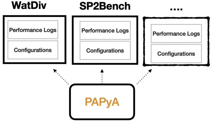
The focus of this paper is to show the internals and functionality of PAPAYA as a means for providing PPA for BD relational systems that query large (RDF) graphs. For completeness, we aim to describe PAPAYA prescriptions with the WatDiv benchmark [5] experiments.33 In [19], we applied Bench-Ranking to the
Fig. 1.
PAPAYA dynamicity.
Outline. Section 2 discusses the related work. Section 3 presents the necessary preliminaries to understand the paper’s content. Section 3.2 briefly introduces the Bench-Ranking framework concepts [19]. Section 4 presents the PAPAYA requirements alongside its framework architecture. Section 5 shows how to use PAPAYA in practice, providing examples from existing experiments [19,21], while Section 6 concludes the paper and presents PAPAYA’s roadmap.
2.Related work
Several tools and recommendation frameworks exist to reduce the effort required to design and execute reproducible experiments, share their results, and build pipelines for various applications [16]. For instance, the RSPLab provides a test-drive for stream reasoning engines that can be deployed on the cloud. It enables the design of experiments via a programmatic interface that allows deploying the environment, running experiments, measuring the performance, and visualizing the results. In their work outlined in [3], the authors tackled the problem of quantifying the continuous behavior of a query engine and presented two novel experimental metrics (dief@t and dief@k) that capture the performance efficiency during an elapsed period rather than a constant time. These metrics evaluate the query engine performance based on the query processing logs at various times (t) and various results (k). On another side, gMark [7] presents a flexible, domain-agnostic, extensible graph dataset generator driven by schemas. Additionally, it furnishes query workloads tailored to anticipated selectivity. Similarly, authors in [6] provide a data loader that facilitates generating RDF graphs in different logical relational schemas and physical partitioning options. However, this tool stops the work of data generation and data loading. This tool leaves the work of deciding the best experimental solutions for the data/knowledge engineers.
The mentioned efforts aim at providing the environment that enables the practitioners to develop their experimental pipelines. Nonetheless, none of these efforts provide prescriptive performance analyses in the context of BD problems. Conversely, PAPAYA aims to cover this timely research gap in an easy and extensible approach, facilitating the building of an experimental solution space for processing large RDF KGs, hence automating PPA where possible.
3.Background
This section presents the necessary background to understand the paper’s content. We assume that the reader is familiar with the RDF data model and the SPARQL query language.
3.1.RDF relational processing experimental dimensions
Several design decisions emerge when utilizing relational BD systems for querying large (RDF) graphs, such as the relational schema, partitioning techniques, and storage formats. These experimental dimensions directly impact the performance of BD systems while querying large graphs. Intuitively, these dimensions entail different choice options (we call them dimensions’ parameters).
First, the relational schema, it is easy to show that we have different options on how to represent graphs as relational tables, and the choice hugely impacts the performance [1,28]. We identify the most used ones in the literature of RDF processing [1,2,27,28]: Single Statement Table (ST) schema that stores RDF triples in a ternary-column relation (subject, predicate, object), and often requires many self-joins; Vertically Partitioned Tables (VP) proposed by Abadi et.al. [1] to mitigate issues of self-joins in ST schema proposing to use binary relations (subject, object) for each unique predicate in the RDF dataset; the Property Tables (PT) schema that prescribes clustering multiple RDF properties as n-ary columns table for the same subject to group entities that are similar in structure. Lastly, two more RDF relational schema advancements also emerge in the literature. The Wide Property Table (WPT) schema encodes the entire dataset into a single denormalized table. WPT is initially proposed for Sempala system by Scätzle et.al. [27], who also proposed another schema optimization that extended the version of the VP schema (ExtVP) [28] that pre-computes semi-join VP tables to reduce data shuffling.
BD platforms are designed to scale horizontally; thus, data partitioning is another crucial dimension for querying large graphs. However, choosing the right partitioning technique for RDF data is non-trivial. To this extent, we followed the indication of Akhter et.al. [4]. In particular, we selected the three techniques that can be applied directly to RDF graphs while being mapped to a relational schema. Namely, (i) Horizontal Partitioning (HP) randomly divides data evenly on the number of machines in the cluster, i.e., n equally sized chunks, where n is the number of machines in the cluster. (ii) Subject-Based Partitioning (SBP) (or (iii) Predicate-Based Partitioning (PBP)) distributes triples to the various partitions according to the hash value computed for the subjects (predicates). As a result, all the triples with the same subject (predicate) reside on the same partition. Notably, both SBP and PBP may suffer from data skewness which impacts parallelism.
Serializing RDF data also offers many options such as RDF/XML, Turtle, JSON-LD, to name a few. On the same note, BD platforms offer many options for reading/writing to various file formats and storage backends. Therefore, we need to consider the variety of storage formats [13]. We specifically focus on the various Hadoop Distributed File System (HDFS) file formats that are suitable for distributed scalable setups. In particular, HDFS supports the following row-oriented formats (e.g., CSV and Avro) and columnar formats (e.g., ORC and Parquet).
3.2.Bench-ranking in a nutshell
This section summarizes the concept of Bench-Ranking as a means for Prescriptive Performance Analysis. Bench-Ranking is based on three fundamental notions, i.e., Configuration, Ranking Function, and Ranking Set, defined below.
Definition 1.
A configuration c is a combination of experimental dimensions. The configuration space
In [19], we consider a three-dimensional configuration space, i.e., including relational schemas, partitioning techniques and storage formats. Figure 2 shows the experimental space and highlights the example of the (a.ii.3) configuration, which is akin to the Single Triples (ST) schema, Subject-based Partitioning (SBP) technique, and stored in the HDFS (ORC) storage file format. This naming convention guides configurations reading in the rest of the paper results (figures and tables).
![The configuration space C [19].](https://content.iospress.com:443/media/sw-prepress/sw--1--1-sw243582/sw--1-sw243582-g002.jpg)
Definition 2.
A ranking set
Definition 3.
A ranking set is defined by a ranking function
A valid example of a ranking score can be the time required for query executions by each of the selected configurations (see Table 1). The ranking function abstracts this notion (Definition 3). In [19], we consider a generalized version of the ranking function presented in [4], which calculates the rank scores for the configurations as follows:
Table 1
Configuration rankings by query execution time, e.g., (a.i.1) configuration is at 41th rank in
| Query | ||||||||
| Conf. | Q1 | Q2 | ... | Q20 | Q1 | Q2 | ... | Q20 |
| a.i.1 | 63.8 | 50.9 | ... | 13.5 | 41th | 41th | ... | 40th |
| a.i.2 | 133.3 | 147.5 | ... | 46.8 | 44th | 48th | ... | 46th |
| ... | ... | ... | ... | ... | ... | ... | ... | ... |
| b.iii.4 | 24.8 | 25.2 | ... | 7.5 | 11th | 26th | ... | 32th |
| ... | ... | ... | ... | ... | ... | ... | ... | ... |
| e.ii.4 | 205.2 | 162.3 | ... | 26.6 | 60th | 60th | ... | 42th |
In Equation (1), R is the rank score of the ranked dimension (i.e., relational schema, partitioning technique, storage format, or any other experimental dimensions). Such that, d represents the total number of parameters (options) under that dimension (for instance five in case of schemas, see Fig. 2),
![Example of rank scores [19]](https://content.iospress.com:443/media/sw-prepress/sw--1--1-sw243582/sw--1-sw243582-g003.jpg)
Despite its generalization, Equation (1) is insufficient for ranking the configurations in a configuration set defined
Finally, our Bench-Ranking frameworks include two evaluation metrics to assess the effectiveness of the proposed ranking criteria. In particular, we consider a ranking criterion is good if it does not suggest low-performing configurations and if it minimizes the number of contradictions within an experimental setting. When it comes to PPA, practitioners are not interested in a configuration that is the fastest at answering any specific query in a workload as long as it is never the slowest at any of the queries. To this extent, we identified two evaluation metrics [19], i.e.,
(i) Conformance, which measures the adherence of the top-ranked configurations w.r.t actual query results (see Table 1);
(ii) Coherence which measures the level of (dis)agreement between two ranking sets that use the same ranking criterion across different experiments (e.g., different dataset sizes).
We calculate the conformance according to Equation (2) by positioning an element in a ranking set w.r.t the initial rank score. For instance, let’s consider a ranking criterion
For coherence, we employ Kendall’s index55 according to Equation (3), which counts the number of pairwise (dis)agreements between two ranking sets, Kendall’s distance between two ranking sets
We assume that ranking sets have the same number of elements. For instance, the K index between
4.PAPAYA
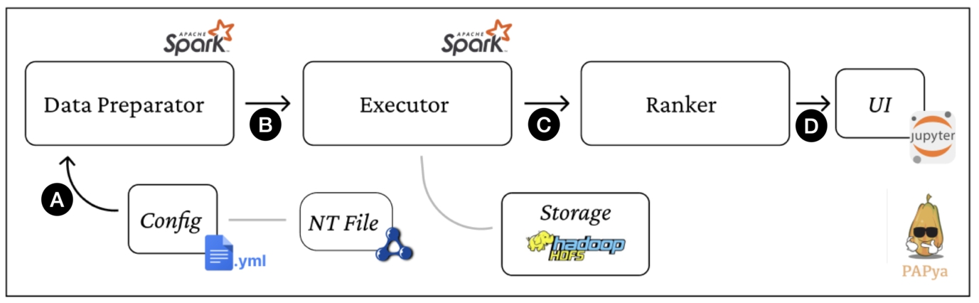
In this section, we present the requirement analysis for PAPAYA library and describe its architecture (Fig. 3). We elicit PAPAYA’s requirements based on the implementation challenges we discussed in the introduction and on the existing research efforts on benchmarking BD systems for processing and querying large RDF graphs [9,19,22,27,28]. Before delving into the requirements, it is also important to list the assumptions under which PAPAYA is designed. We derive the following assumptions from our work on the Bench-Ranking framework [19].
Fig. 3.
Papaya architecture and workflow.
A.1 Posthoc Performance Analysis of One-Time Query Processing: Bench-Ranking framework [19], wrapped in PAPAYA, only supports “One-Time” query processing of SPARQL queries mapped into SQL and runs on top of big relational management systems (e.g., Spark-SQL). This excludes the performance analyses done for continuous query processing [3].
A.2 Query workload includes only Conjunctive SPARQL SPJ queries: The query workload includes only Conjunctive SPARQL Select-Project-Join (SPJ) queries for which there exists an SQL translation for a given schema.
A.3 Query Engine is a black box: In PAPAYA, The query engine is treated as a black box, and thus the “pre-processing” query optimization phase is not part of the analysis. The query optimization is delegated to the Big data management systems’ optimizers (e.g., SparkSQL Catalyst).
4.1.Requirements
Given our assumptions, we can outline the requirements as follows:
R.1 Support for PPA: PAPAYA shall support the necessary abstractions required to support PPA. Moreover, by default, it shall support existing Bench-Ranking techniques in [19]. (O.0)
R.2 Independence from the Key Performance Indicators (KPIs): PAPAYA must enable PPA independently from the chosen KPI. In [19], we opted for query latency, yet one may need to analyze the performance in terms of other metrics (e.g., memory consumption). (O.2)
R.3 Independence from Experimental Dimensions: PAPAYA must allow the definition of an arbitrary number of dimensions, i.e., allow the definition of n-dimensional configuration space. (O.3)
R.4 Usability: PAPAYA prepares the experimental environment for processing large RDF datasets. Also, it supports decision-making, simplifying the performance data analytics. To this extent, data visualization techniques and a simplified API are both of paramount importance. (O.0)
R.5 Flexibility and Extensibility: PAPAYA should be extensible both in terms of architecture and programming abstractions to adapt to adding/removing configurations, dimensions, workload queries, ranking methods, evaluation metrics, etc. It also should decouple data and processing abstractions to ease the integration of new components, tools, and techniques. (O.1, O.3)
4.2.Architecture, abstractions, and internals
This section presents the PAPAYA’s main components and shows how they fulfill the requirements. Table 3 summarizes the requirements for challenges mappings alongside the PAPAYA solutions. PAPAYA allows its users to build an entire pipeline for querying big RDF datasets and analyzing the performance results. In particular, it facilitates building the experimental setting considering the configuration space (described in Definition 1) specified by users. This entails preparing and loading the graph data in a user-defined relational configuration space, then performing experiments (executing a query workload on top of a relational BD framework), and finally analyzing and providing prescriptions of the performance.
Table 3
Summary of challenges and requirements mapping along with PAPAYA solutions
| Challenges | Requirements | PAPAYA solutions |
| C.1: Experiments Preparation | R4, R5 | – Data Preparator that generates and loads graph data for distributed relational setups. |
| – User-defined YAML configurations files. | ||
| C.2: Portability and Usability | R2, R3, R4, R5 | – Data Preperator prepares graphs data ready for processing with any arbitrary relational BD system. |
| – Internals & abstractions enable plugin-in new modules and programmable artifacts. | ||
| – Checking performance replicability whilst configuration changes. | ||
| C.3: Flexibility and Extensibility | R1, R3, R5 | – Allow adding/excluding experimental dimensions. |
| – Allow adding new ranking algorithms. | ||
| – Flexibility in shortening and enlarging the configuration space. | ||
| C.4: Compoundness and Complexity | R1, R4 | – Interactive Jupyter Notebooks. |
| – Variety of data and ranking visualizations |
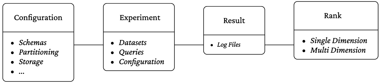
To achieve that, PAPAYA includes three core modules depicted in Fig. 3, i.e., the Data Preparator, the Executor, and the Ranker. Moreover, PAPAYA relies on few core abstractions depicted in Fig. 4, i.e., Configuration, Experiment, Result, and Rank. While detailing each module’s functionalities, we introduce PAPAYA workflow, which also appears in Fig. 3, starting with the input is a configuration file that points to the input N-Triple file with the RDF graph (Fig. 3 step (A)).
Fig. 4.
PAPAYA internal abstractions.
The first actor in the pipeline is the Data Preparator (DP), which prepares RDF graphs for relational processing. It takes as input a configuration file that includes experimental options of interest. The configuration file is represented by the Configuration abstraction (see Fig. 4), which enables extensibility (R.5). Specifically, the DP allows defining an arbitrary number of dimensions with as many options as specified (R.3). In particular, it considers the dimensions specified in [19] (R.1), i.e., relational schemas, storage format, and partitioning technique. Therefore, the DP automatically prepares (i.e., determines, generates, and loads) the RDF graph dataset with the specified configurations that adapt with the relational processing paradigm to the storage destination (e.g., HDFS). More specifically, DP currently includes four relational schemas commonly used for RDF processing, i.e., (a) ST, (b) VP, (d) ExtVP, and (e) WPT.66 For partitioning, DP currently supports three partitioning techniques, i.e., (i) horizontal partitioning (HP), (ii) subject-based partitioning (SBP), and predicate-based partitioning (PBP). Last but not least, DP enables storing data using four HDFS file formats (i) CSV or (ii) Avro, which are row-oriented, and (iii) ORC or (iv) Parquet, which are column-oriented storage formats [13].
The DP interface is generic, and the generated datasets are agnostic to the underlying relational system. The DP prepares RDF graph data for processing with different relational BD systems, especially SQL-on-Hadoop systems, e.g., SparkSQL, Hive, and Impala. Seeking scalability, the current DP implementation relies on SparkSQL, which allows implementation of RDF relational schema generation using the SQL transformations. Notably, Apache Hive or Apache Impala could be potential candidates for alternative implementation executors. However, SparkSQL also supports different partitioning techniques and multiple storage formats, making it ideal for our experiments [19].
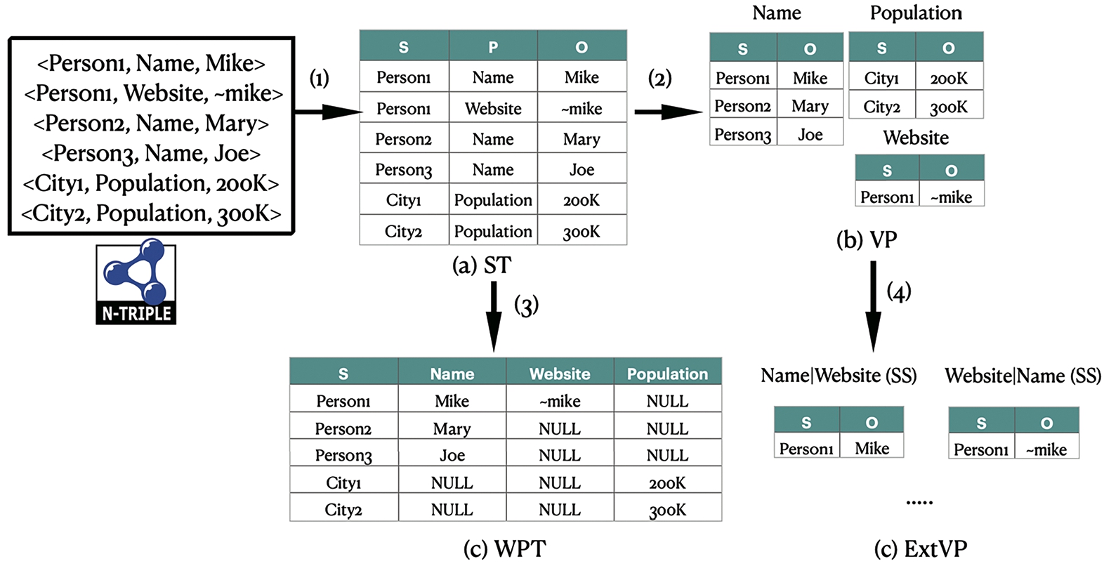
Figure 5 shows a sample of schema generation in PAPAYA DP component. First, the DP transforms the input RDF graph (N-Triples file(s)) into an ST table schema (i.e., Fig. 5 Step (1)), and then other schemas are generated using parameterized SQL queries.77 For instance, the VP and WPT schemas are generated using SQL queries given the ST table as a parameter (i.e., Fig. 5 Step (2), and (3), respectively). While, the ExtVP schema generation relies on VP tables to exist first (i.e., Step (4) in Fig. 5).
Fig. 5.
RDF relational schema transformations in PAPAYA data preparator.
The Executor is the following module in PAPAYA workflow, which is the system that is subject to experimentation (see Fig. 3 step B). For instance, in [9,19,21,28] the considered system is Apache SparkSQL. The executor offers an abstract API to be extended (R.5). In practice, it (i) starts the execution pipeline in the external system, (ii) it collects the performance logs (R.2), and currently, it persists them on a file system, e.g., HDFS. The Executor expects a set of experiments to run defined in terms of (i) a set of queries, (ii) an RDF dataset (size), and (iii) a configuration (defined in Definition 1). The Experiment abstraction is defined in Fig. 4. We decided to wrap the running experiments in a SparkSQL-based executor (SparkExecutor). The experiment specifications (alongside the configurations) are passed to this wrapper as parameters. It is worth mentioning that the Executor assumes the query workload is available in the form of SQL queries (Assumption A.2) running in a “One-Time” style [3] (Assumption A.1). In the current stage, PAPAYA does not support SPARQL query translation nor SQL query mappings, this work is left for the future roadmap of PAPAYA (see Section 6). It is also important to note that the current version of PAPAYA delegates the query optimization to the executor’s optimizer (Assumption A.3).
The results logs are then loaded by the Ranker component into python Dataframes to make them available for analysis (see Fig. 3 step (C)). The Ranker reduces the time required to calculate the rankings, obtain useful data visualizations, and determine the best-performing configurations while checking the performance replicability. To fulfill R.2, i.e., the Ranker component operates over a log-based structure whose schema shall be specified by the user in the input configurations. Moreover, to simplify the usage and the extensibility (R.5), we decoupled the performance analytics (e.g., ranking calculation) from its definitions and visualization. In particular, the Rank class abstraction reflects on the ranking function (Definition 3) that takes as input data elements and returns a ranking set. To fulfill R.4, a default data visualization for the rank shall be specified. However, this is left for the user to specify due to the specificity of the visualization.
The Rank call allows defining additional ranking criteria (R.5). In addition, to fulfill R.1, PAPAYA already implements SD as well as Multi-Dimensional (MD) criteria specified in [19].
PAPAYA allows its users to interact with the experimental environment (R.5) using Jupyter Notebook. To facilitate the analysis, it integrates data visualization (R.4) that can aid decision-making. Thus, the Rank class includes a specific method to implement, where to specify the default visualization.
Finally, to evaluate the raking criteria, we introduced in Section 3.2 the notions of coherence and conformance (R.1). Ranking criteria evaluation metrics are employed to select which ranking criterion is “effective” (i.e., if it is not suggesting low-performing configurations). In our experiments, we use such metrics by looking at all ranking criteria and comparing them with the results across different scales, e.g., dataset sizes (
5.PAPAYA in practice
In this section, we explain how to use PAPAYA in practice, showcasing its functionalities with a focus on performance data analysis, flexibility, and visualizations. In particular, we design our experiments in terms of (i) a set of SPARQL queries that we manually translated into SQL accordingly with the different relational schemas, (ii) RDF datasets of different sizes automatically prepared using our Spark-based DataPreparator, and (iii) a configuration based on three dimensions as in [19], i.e., schema, partitioning techniques, and storage formats.
In Bench-Ranking experiments [19], we used the
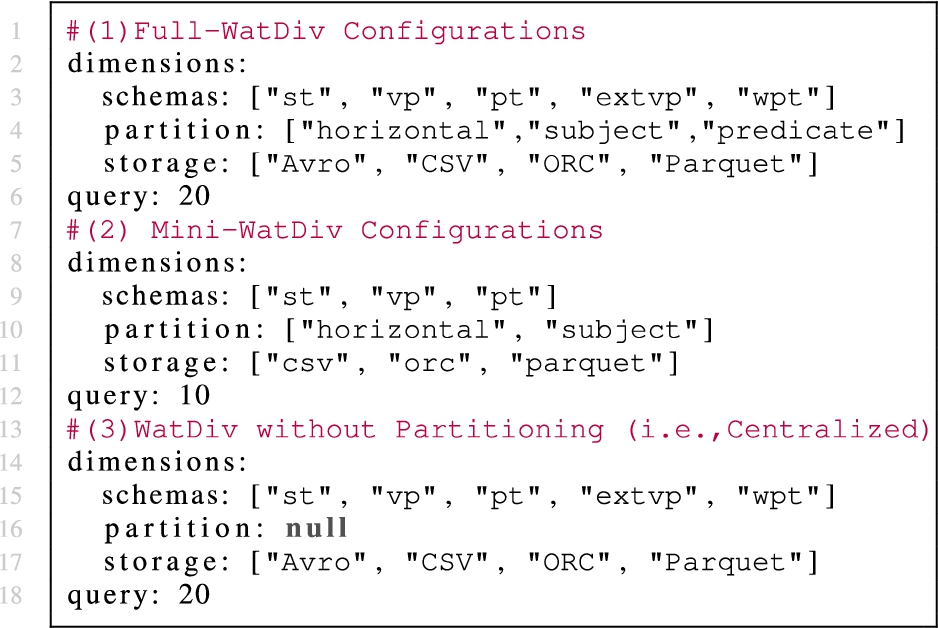
Listing 1 shows a full example of PAPAYA pipeline, starting by deciding the configurations (in terms of three dimensions and their options, e.g., list of schemas, partitioning techniques, storage formats to prepare, load, and benchmark) (Listing 1 lines 4–8). Then, an experiment is set up for running, defining the dataset size (e.g., “100M” triples), a list of queries to execute or exclude from the workload, and the configurations (Listing 1 line 10). An executor is defined for running the experiment along with the number of times experiments will be run (Listing 1 line 11). The results (runtime logs) are kept in log files in a specified path (e.g., HDFS or a local disk). The Bench-Ranking phase starts when we have the results in logs (Listing 1 line 13).1010 For instance, we call the SDRank (Listing 1 line 15) for calculating rank scores for the “schema” dimension, alongside specifying the number of queries (“q”), and number of options under this dimension (“d” in Equation (1)). The MD-Ranking(i.e., Pareto fronts) is applier in two ways. The first one is called
Listing 1.
Experiment design example in PAPAYA
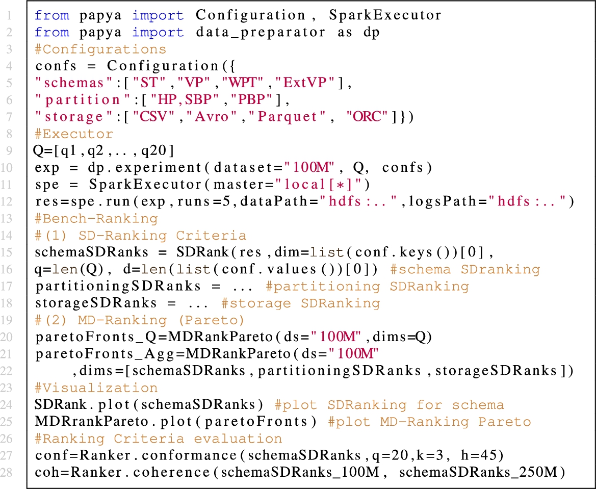
Table 4 shows the top-3 ranked configuration according to the various ranking criteria, i.e., Single-Dimension and Multi-Dimensional (Pareto) for the WatDiv datasets (i.e., 100M, 250M, 500M triples). In addition, Table 5 provides the ranking evaluation metrics (calculated according to Equations (2) and (3)).
Table 4
WatDiv best-performing (Top-3) configurations according to the SD and MD ranking criteria
| a.ii.3 | a.ii.3 | c.i.4 | c.ii.2 | a.ii.3 | a.ii.3 | a.ii.3 | c.ii.2 | d.iii.4 | d.iii.2 | c.ii.2 | c.ii.2 | |
| b.ii.2 | a.ii.4 | c.ii.2 | c.i.2 | c.ii.2 | c.ii.2 | a.i.3 | b.iii.3 | d.iii.1 | d.iii.3 | d.iii.3 | d.iii.3 | |
| a.i.3 | a.ii.2 | c.i.3 | b.ii.2 | b.ii.2 | b.ii.2 | b.ii.2 | c.ii.1 | d.iii.3 | d.iii.4 | b.ii.2 | b.ii.2 | |
| a.ii.3 | a.ii.3 | c.i.4 | c.i.4 | c.i.4 | c.i.4 | a.ii.3 | a.ii.1 | d.iii.4 | d.iii.2 | d.iii.3 | d.iii.3 | |
| a.i.3 | a.ii.4 | c.i.3 | c.ii.2 | b.ii.2 | b.ii.2 | a.i.3 | d.iii.3 | d.iii.3 | d.iii.3 | c.i.4 | c.i.4 | |
| c.i.4 | a.ii.2 | c.i.2 | c.i.2 | a.ii.3 | a.ii.3 | b.iii.2 | a.ii.2 | d.iii.2 | c.i.4 | a.iii.4 | a.iii.4 | |
| a.ii.3 | a.ii.3 | c.ii.4 | c.ii.3 | b.ii.2 | b.ii.2 | a.ii.3 | c.ii.2 | d.iii.2 | d.ii.2 | d.ii.2 | c.ii.3 | |
| a.i.3 | a.ii.4 | c.i.4 | c.ii.4 | c.ii.3 | c.ii.3 | a.i.3 | a.iii.2 | d.iii.4 | c.ii.3 | c.ii.3 | d.ii.2 | |
| c.i.3 | a.ii.2 | c.i.3 | c.i.3 | c.ii.4 | c.ii.4 | c.iii.2 | a.iii.4 | d.iii.1 | a.iii.4 | a.iii.4 | a.iii.4 | |
Table 5
Ranking coherence (Kendall distance, the lower the better) & conformance across WatDiv datasets (D1=100M, D2=250M, D3=500M)
| WatDivMini | WatDifull | |||||||||||
| Conformance | Coherence | Conformance | Coherence | |||||||||
| D1 | D2 | D3 | D1–D2 | D1–D3 | D2–D3 | D1 | D2 | D3 | D1–D2 | D1–D3 | D2–D3 | |
| 88.33% | 91.67% | 93.33% | 0.09 | 0.12 | 0.06 | 96.00% | 94.00% | 93.00% | 0.1 | 0.13 | 0.07 | |
| 38.33% | 13.33% | 5.00% | 0.14 | 0.14 | 0.14 | 73.00% | 39.00% | 36.00% | 0.09 | 0.28 | 0.17 | |
| 63.33% | 46.67% | 35.00% | 0.16 | 0.39 | 0.3 | 64.00% | 32.00% | 43.00% | 0.14 | 0.25 | 0.15 | |
| 95.00% | 98.33% | 95.00% | 0.14 | 0.25 | 0.14 | 92.00% | 98.00% | 98.00% | 0.1 | 0.15 | 0.07 | |
| 88.33% | 73.33% | 93.33% | 0.16 | 0.25 | 0.2 | 87.00% | 71.00% | 76.00% | 0.17 | 0.24 | 0.15 | |
| 88.33% | 73.33% | 93.33% | 0.2 | 0.24 | 0.17 | 89.00% | 84.00% | 76.00% | 0.15 | 0.22 | 0.13 | |
5.1.Rich visualizations
To fulfill R.4, PAPAYA decouples data analytics from visualizations. Meaning that the user can specify his/her visualizations of interest with the performance data. Nevertheless, PAPAYA still provides several interactive and extensible default visualizations that help practitioners rationalize the performance results and final prescriptions. In addition, visualizations are simple and intuitive for understanding several Bench-Ranking definitions, equations, and evaluation metrics. For instance, Fig. 6 (a-c) shows three samples of SD-ranking criteria plots. In particular, they show how many times a specific dimension’s (e.g., the schema in Fig. 6 (a)) alternatives/options (ST, VP, PT,..etc) achieve the highest or the lowest ranking scores. Figure 7 shows the SD ranking criteria w.r.t a simple geometrical representation (detailed in the following sections) that depicts the triangle subsumed by each dimension’s ranking criterion (i.e., Rs, Rp, and Rf). The triangle sides present the trade-off ranking dimensions and show that the SD-ranking criteria may only optimize towards a single dimension at a time. The MD-ranking criteria, i.e.,
Fig. 6.
Examples on SD rank scores over different dimensions (100M), the higher the better.
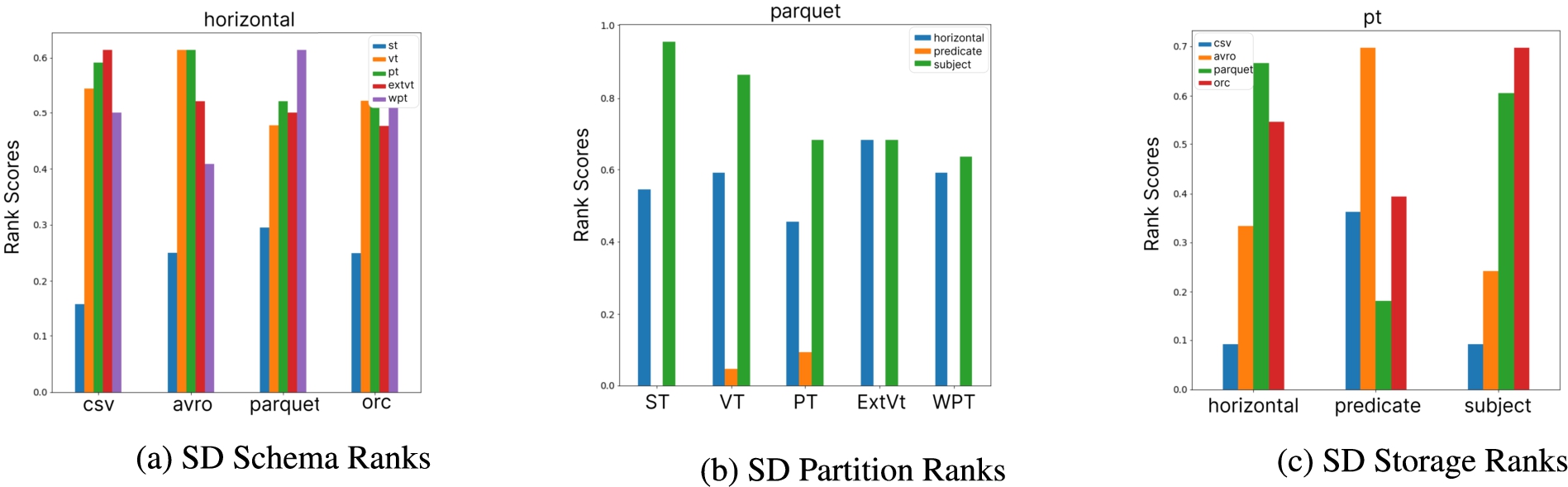
Fig. 7.
Dimensions trade-offs using single-dimensional ranking (
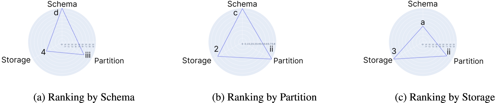
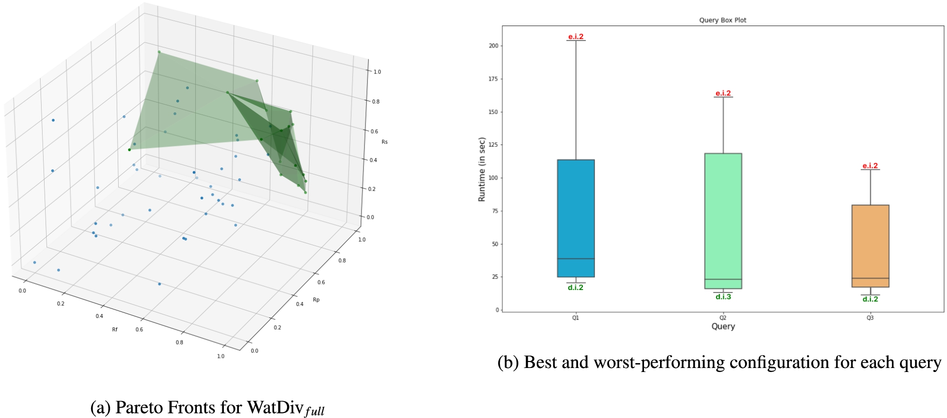
Fig. 8.
Pareto fronts, and queries best-worst configuration examples.
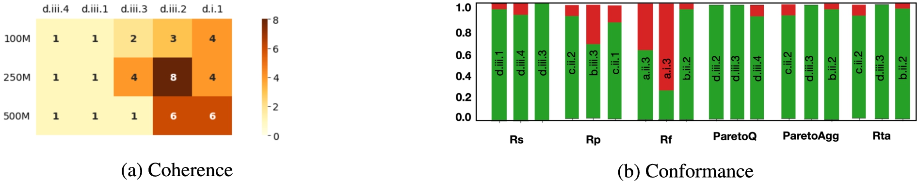
PAPAYA visualizations allow explaining the conformance and coherence results using simple plots. For instance, Fig. 9 (a) shows the coherence of the top-5 ranked configurations of the Rs criterion in the 100M dataset while scaling to the larger datasets, i.e., 250M and 500M. PAPAYA explains the conformance of the Bench-Ranking criteria by visualizing the conformance of the top-3 ranked configurations (or any arbitrary number of configurations) with the actual query rankings (Table 1). The green color represents the level of conformance, and the red depicts a configuration that is performing worse than the h worst rankings. Thus, this may explain why
Fig. 9.
Heatmap shows the coherence of the
Practitioners can also use PAPAYA visualizations for fine-grained ranking details. For instance, showing the best and worst configurations for each query (as shown in Fig. 8 (b) for example of three queries of the WatDiv workload). Such detailed visualizations could help the user rationalize the final prescriptions of PAPAYA.
5.2.PAPAYA flexibility & extensibility
Adding/Removing Configurations/Queries.
Listing 2.
YAML configuration file for various experiments in PAPAYA
To show an example of the extensibility of PAPAYA, we implement the Bench-Ranking criteria over a subset of the configurations and subset of the WatDiv benchmark tasks (i.e., queries); we call it
The right side of Table 4 shows the top-ranked three configurations according to the specified configurations. Intuitively, results differ according to the available ranked configuration space. For instance, with the inclusion of the ExtVP schema (i.e., ‘d’), it dominates instead of the PT schema (i.e., ‘c’) in
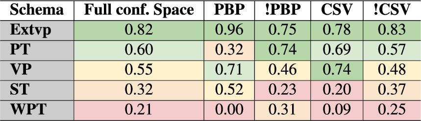
With such flexibility, PAPAYA also provides several dynamic views on the ranking criteria. For example, Table 6 shows the SD ranking of the schema dimension by changing the configuration space. Particularly, it shows how the global ranking of each relational schema (or any other specified dimension) could change by including/excluding configurations of the other dimensions. The table shows that the order of the global schema ranks changes by including all configurations (“Full Conf. Space”) than including/excluding the predicate partitioning or CSV format, i.e., “PBP/!PBP”, “CSV/!CSV”, respectively. For instance, the PT schema global ranking is interestingly oscillating with those changes in the available configurations.
Table 6
Schemas global ranking across various configurations
Adding/Removing Full Experimental Dimension. PAPAYA’flexibility extends to the experimental dimensions, i.e., it is possible to add/remove dimensions easily. For instance, we can fully exclude the partitioning dimension in case experiments are executed on a single machine (see Listing 2 lines 13–18). In [23], we run experiments on SparkSQL with different relational schemas and storage backends yet without data partitioning. Table 7 shows the best-performing (top-3) configurations in WatDiv experiments when excluding the partitioning dimension. Table 8 shows the conformance and coherence metrics’ results for the various ranking criteria.1313
Table 7
Best-performing configurations, excluding the partitioning dimension
| 100M | d.i.1 | a.i.3 | c.i.2 | c.i.2 |
| c.i.2 | b.i.2 | d.i.2 | b.i.2 | |
| d.i.2 | e.i.4 | d.i.4 | d.i.1 | |
| 250M | c.i.1 | a.i.3 | d.i.2 | d.i.2 |
| d.i.2 | e.i.4 | c.i.4 | c.i.1 | |
| c.i.3 | d.i.2 | c.i.2 | e.i.4 | |
| 500M | d.i.2 | a.i.3 | d.i.2 | d.i.2 |
| c.i.3 | d.i.2 | c.i.3 | a.i.3 | |
| c.i.1 | e.i.4 | c.i.4 | c.i.3 |
Table 8
Criteria evaluation (conform.ance, and coher.ence), excluding partitioning
| Metric | D | ||||
| Conform. | 100M | 97.50% | 67.50% | 95.00% | 92.50% |
| 250M | 97.50% | 30.00% | 100.00% | 97.50% | |
| 500M | 100.00% | 52.50% | 100.00% | 52.50% | |
| Cohere. | 100M–250M | 0.11 | 0.17 | 0.11 | 0.19 |
| 100M–500M | 0.28 | 0.16 | 0.30 | 0.18 | |
| 250M–500M | 0.17 | 0.08 | 0.15 | 0.09 |
Adding Ranking Criterion. PAPAYA abstractions enable users to plug in a new ranking criterion besides the already existing ones (i.e., the abstract Rank class, Section 4). Let’s assume we seek usage of a simple ranking criterion that leverages a geometric interpretation of the SD rankings of the three experimental dimensions based on the triangle area subsumed by each ranking criterion (
In Fig. 10, the triangle sides represent the SD-ranking dimensions’ rank scores. Thus, this criterion aims to maximize this triangle’s area (i.e., the blue triangle). The closer to the ideal (outer red triangle), the better it scores. In other words, the bigger the area of this triangle covers, the better the performance of the three ranking dimensions altogether. The red triangle represents the case with the maximum/ideal rank score, i.e.,
Fig. 10.
Triangle area criterion.
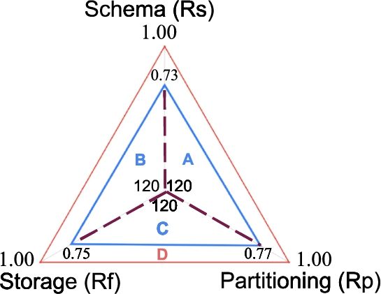
The formula (Cf. Equation (4)) computes the actual triangle area. Simply, it sums up the triangle area of the three triangles A, B, and C by two of its sides which are the rank scores of each dimension, i.e.,
Listing 3.
Plugin the triangle-area as new ranking criterion
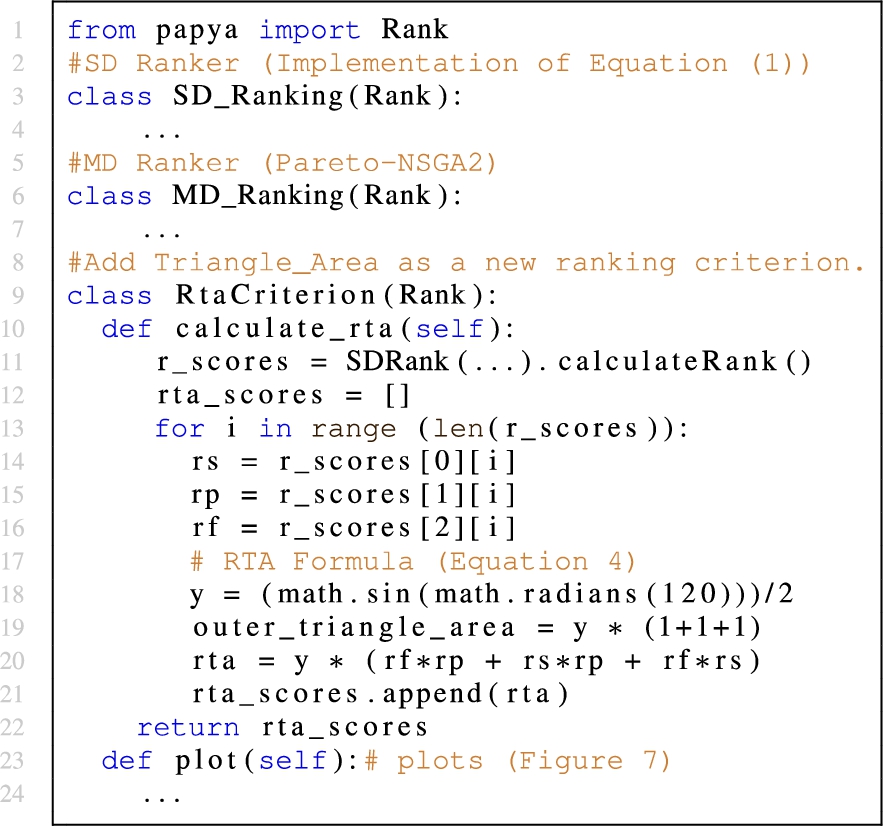
It is worth mentioning that the idea behind
5.3.Checking performance replicability
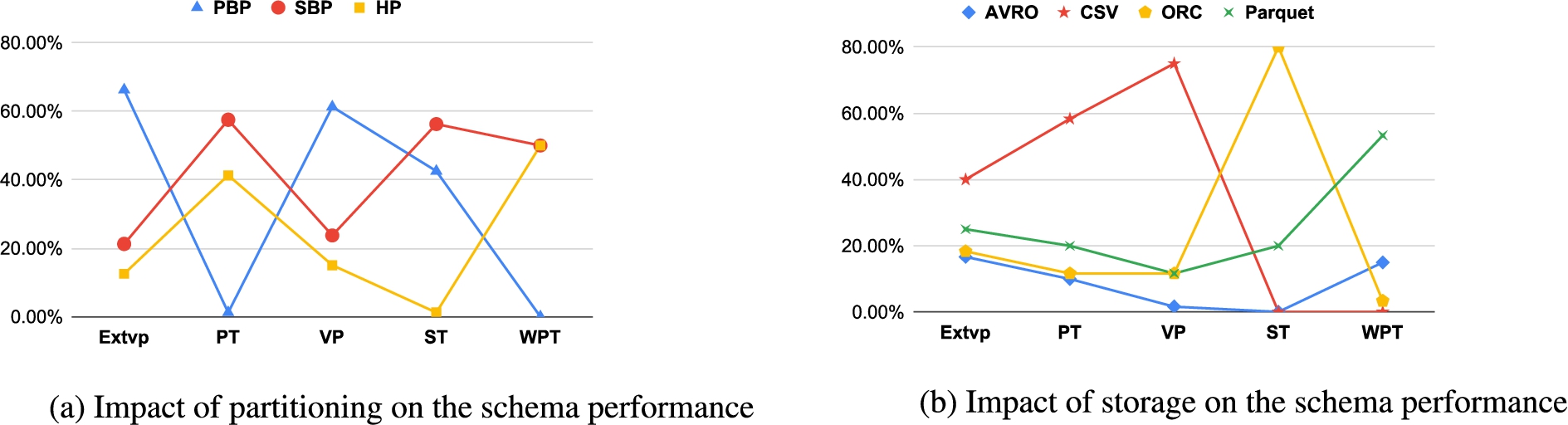
PAPAYA also activates the functionality of checking the BD system’s performance replicability when introducing different experimental dimensions. In particular, it enables checking the system’s performance with one specific dimension while changing the parameters of the other dimensions. For example, Figs 11 (a) and (b) respectively show the impact of the partitioning and storage on the performance of the schema dimension. The Figures show how the performance of the system with a configuration can significantly change with changing other dimensions.
Fig. 11.
Schema replicability across changing partitioning or storage formats.
PAPAYA can also check the performance replicability by comparing two configurations as discussed in [21]. For instance, PAPAYA can compare the schema optimizations (i.e., WPT, and ExtVP) w.r.t their baseline ones (i.e., PT, and VP) while introducing different partitioning techniques and various HDFS storage formats that are different from the baseline configurations [27,28].
Table 9 shows the effect of introducing partitioning techniques (right of the table) and different file formats (left of the table) different from the baseline configurations (i.e., Vanilla HDFS partitioning and Parquet as storage format). The trade-offs effect is evident in the replicability results. Indeed, WPT outperforms PT schema only with
Table 9
The replicability of schema advancements (i.e., WPT, ExtVP) VS. baselines (i.e., PT, VP), WatDiv 500M dataset
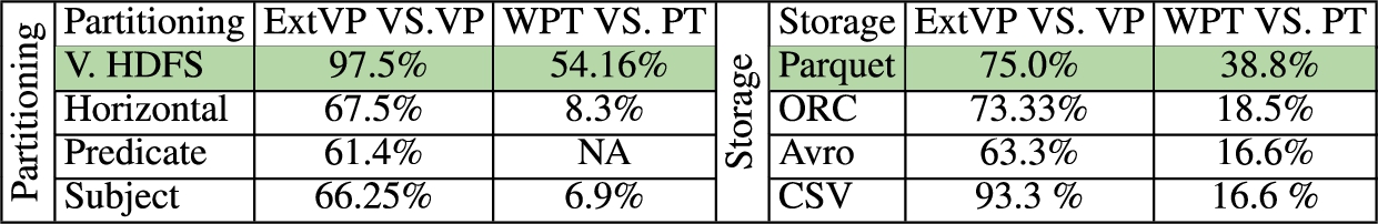
Table 10 provides a concise overview of the objectives, delineating the challenges encountered during their pursuit, and outlines the set of requirements necessary for accomplishing these objectives.
6.Conclusion and roadmap
Table 10
Summary of objectives, challenges, and requirements
| Objectives | Challenges | Requirements |
| O.0 | C.1, C.2 | R.2–R.5 |
| O.1 | C.2, C.3 | R.1–R.5 |
| O.2 | C.2, C.3, C.4 | R.1–R.5 |
| O.3 | C.2, C.3, C.4 | R.1–R.5 |
This paper presents PAPAYA, an extensible library that reduces the efforts needed to analyze the performance of BD systems used for processing large (RDF) graphs. PAPAYA implements the performance analytics methods adopted in [23,27,28] including an novel approach for prescriptive performance analytics we presented in [19].
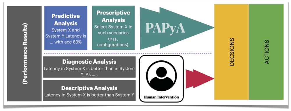
Inspired by Gartner’s analysis methodology [11], Fig. 12 reflects the amount of human intervention required to make a decision with the descriptive and diagnostic analyses of the performance results. Descriptive and diagnostic analytics are limited, and cannot guide practitioners directly to the best-performing configurations in a complex solution space. This is shown in this paper with the lack of performance replicability (shown Section 5.3). Indeed, the performance of the BD system is affected by changing the configurations, e.g., oscillating schema performance with changing partitioning, and storage options (Fig. 11). On the other side, PAPAYA aims to reduce the amount of work required to interpret performance data. It adopts the Bench-ranking methodology with which practitioners can easily decide the best-performing configurations given an experimental solution space with an arbitrary number of dimensions. Although descriptive discussions are limited, PAPAYA still provides several descriptive analytics and visualizations on the performance to explain the final decisions given by PAPAYA. PAPAYA also aims to reduce the engineering work required for building an analytical pipeline for processing large RDF graphs. In particular, PAPAYA prepares, generates, and loads data ready for big relational RDF graph analytics.
Fig. 12.
Performance analysis methodology, and how PAPAYA reduces human intervention in BD analytics.
PAPAYA is developed considering the ease of use and the flexibility aspects allowing extending the library with an additional arbitrary number of experimental dimensions to the solution space. Moreover, PAPAYA provides abstractions on the level of ranking criteria, meaning that the user can use his/her ranking functions for ranking the solution space. Seeking availability, we provide PAPAYA as an open-source library under MIT license and published at a persistent URI. PAPAYA’s GitHub repository includes tutorials and documentation on how to use the library.
As a maintenance plan, PAPAYA’s roadmap includes:
1. Covering the phase of query evaluation into PAPAYA pipeline. In particular, we plan to provide native support of SPARQL by incorporating native triple stores for query evaluation.
2. Incorporating SPARQL into SQL translation for a given schema, i.e., query translation is a schema-dependent task. This can be approached using advancements of R2RML mapping tools (e.g., OnTop) [8].
3. Wrapping other SQL-on-Hadoop executors to PAPAYA; thus, the performance of the engines could also be compared as well as enabling benchmarking of other KG data models (e.g., property graphs [17]) in PAPAYA.
4. Using orchestration tools (such as Apache Airflow) to monitor the PAPAYA pipelines.
5. Integrating PAPAYA with tools like gmark [7], which generates graphs and workloads, and ESPRESSO [20], which enables search and query functionalities over personal online datastores as well as personal KGs.
Notes
2 Cleaning Big Data: Most Time-Consuming, Least Enjoyable Data Science Task, Survey Says https://shorturl.at/wAQ47.
3 Due to space limits, we diagnose the WatDiv prescriptions results and evaluation metrics in Section 5 on the library GitHub page, mentioned below.
4 Pareto frontier aims at finding a set of optimal solutions if no objective can be improved without sacrificing at least one other objective.
5 Kendall is a standard measure to compare the outcomes of ranking functions.
6 Automating PT schema (“b” in Fig. 2) generation is not yet supported by the current PAPAYA DP.
7 schema SQL-based transformations are kept in the DP module on PAPAYA’s GitHub repository due to space limits.
8 Nonetheless, seeking conciseness, we keep
9 Benchmarks’ query workload (in SQL) and experiments runtimes: https://datasystemsgrouput.github.io/SPARKSQLRDFBenchmarking.
10 It is worth noting that the performance analyses, e.g., Bench-Ranking, could start directly if the performance data (logs) are already present.
11
12 Due to space limits, we keep other Pareto figures on the PAPAYA GitHub page.
13 Notably, the Rp and Rta criteria cannot be calculated when excluding the partitioning dimension.
Acknowledgements
We acknowledge support from the European Social Fund via IT Academy programme and the European Regional Development Funds via the Mobilitas Plus programme (grant MOBTT75).
References
[1] | D.J. Abadi, A. Marcus, S.R. Madden and K. Hollenbach, Scalable semantic web data management using vertical partitioning, in: VLDB, (2007) . |
[2] | I. Abdelaziz, R. Harbi, Z. Khayyat and P. Kalnis, A survey and experimental comparison of distributed SPARQL engines for very large RDF data, in: Proceedings of the VLDB Endowment, (2017) . |
[3] | M. Acosta, M.-E. Vidal and Y. Sure-Vetter, Diefficiency metrics: Measuring the continuous efficiency of query processing approaches, in: International Semantic Web Conference, (2017) , pp. 3–19. |
[4] | A. Akhter, A.-C.N. Ngonga and M. Saleem, An empirical evaluation of RDF graph partitioning techniques, in: European Knowledge Acquisition Workshop, (2018) . |
[5] | G. Aluç, O. Hartig, M.T. Özsu and K. Daudjee, Diversified stress testing of RDF data management systems, in: International Semantic Web Conference, Springer, (2014) , pp. 197–212. |
[6] | V.A.A. Ayala and G. Lausen, A flexible N-triples loader for hadoop, in: International Semantic Web Conference (P&D/Industry/BlueSky), (2018) . |
[7] | G. Bagan, A. Bonifati, R. Ciucanu, G.H. Fletcher, A. Lemay and N. Advokaat, gMark: Schema-driven generation of graphs and queries, IEEE Transactions on Knowledge and Data Engineering 29: (4) ((2016) ), 856–869. doi:10.1109/TKDE.2016.2633993. |
[8] | M. Belcao, E. Falzone, E. Bionda and E.D. Valle, Chimera: A bridge between big data analytics and semantic technologies, in: International Semantic Web Conference, Springer, (2021) , pp. 463–479. |
[9] | M. Cossu, M. Färber and G. Lausen, Prost: Distributed execution of SpaRQL queries using mixed partitioning strategies, (2018) , arXiv preprint arXiv:1802.05898. |
[10] | K. Deb, A. Pratap, S. Agarwal and T. Meyarivan, A fast and elitist multiobjective genetic algorithm: NSGA-II, IEEE Transactions on Evolutionary Computation 6: (2) ((2002) ), 182–197. doi:10.1109/4235.996017. |
[11] | J. Hagerty, Planning Guide for Data and Analytics, (2017) , [Online; accessed, 4-Sep-2021]. |
[12] | et al., SPˆ 2Bench: A SPARQL performance benchmark, in: ICDE 2009, Y.E. Ioannidis, D.L. Lee and R.T. Ng, eds, (2009) , pp. 222–233. |
[13] | T. Ivanov and M. Pergolesi, The impact of columnar file formats on SQL-on-hadoop engine performance: A study on ORC and Parquet, Concurrency and Computation: Practice and Experience ((2019) ), e5523. |
[14] | K. Lepenioti, A. Bousdekis, D. Apostolou and G. Mentzas, Prescriptive analytics: Literature review and research challenges, International Journal of Information Management 50: ((2020) ), 57–70. doi:10.1016/j.ijinfomgt.2019.04.003. |
[15] | M.R. Moaawad, H.M.O. Mokhtar and H.T. Al Feel, On-the-fly academic linked data integration, in: Proceedings of the International Conference on Compute and Data Analysis, (2017) , pp. 114–122. doi:10.1145/3093241.3093276. |
[16] | M.R. Moawad, M.M.M.Z.A. Maher, A. Awad and S. Sakr, Minaret: A recommendation framework for scientific reviewers, in: The 22nd International Conference on Extending Database Technology (EDBT), (2019) . |
[17] | M. Ragab, Large scale querying and processing for property graphs, in: DOLAP@EDBT/ICDT 2020, Copenhagen, Denmark, March 30, 2020, (2020) . |
[18] | M. Ragab, Towards prescriptive analyses of querying large knowledge graphs, in: New Trends in Database and Information Systems – ADBIS 2022 Short Papers, Doctoral Consortium and Workshops: DOING, K-GALS, MADEISD, MegaData, SWODCH, Turin, Italy, September 5–8, 2022, Proceedings, S. Chiusano, T. Cerquitelli, R. Wrembel, K. Nørvåg, B. Catania, G. Vargas-Solar and E. Zumpano, eds, Communications in Computer and Information Science, Vol. 1652: , Springer, (2022) , pp. 639–647. doi:10.1007/978-3-031-15743-1_59. |
[19] | M. Ragab, F.M. Awaysheh and R. Tommasini, Bench-ranking: A first step towards prescriptive performance analyses for big data frameworks, in: 2021 IEEE International Conference on Big Data (Big Data), IEEE Computer Society, Los Alamitos, CA, USA, (2021) , pp. 241–251. doi:10.1109/BigData52589.2021.9671277. |
[20] | M. Ragab, Y. Savateev, R. Moosaei, T. Tiropanis, A. Poulovassilis, A. Chapman and G. Roussos, ESPRESSO: A framework for empowering search on decentralized web, in: International Conference on Web Information Systems Engineering, Springer, (2023) , pp. 360–375. |
[21] | M. Ragab, R. Tommasini, F.M. Awaysheh and J.C. Ramos, An in-depth investigation of large-scale RDF relational schema optimizations using spark-SQL, in: Processing of Big Data (DOLAP) Co-Located with the 24th (EDBT/ICDT 2021), Nicosia, Cyprus, (2021) . |
[22] | M. Ragab, R. Tommasini, S. Eyvazov and S. Sakr, Towards making sense of spark-SQL performance for processing vast distributed RDF datasets, in: Proceedings of the International Workshop on Semantic Big Data@ Sigmod’20, New York, NY, USA, (2020) . ISBN 9781450379748. |
[23] | M. Ragab, R. Tommasini and S. Sakr, Benchmarking spark-SQL under alliterative RDF relational storage backends, in: QuWeDa@ ISWC, (2019) , pp. 67–82. |
[24] | M. Ragab, R. Tommasini and S. Sakr, Comparing schema advancements for distributed RDF querying using SparkSQL, in: Proceedings of the ISWC 2020 Demos and Industry Tracks, CEUR Workshop Proceedings, Vol. 2721: , CEUR-WS.org, (2020) , pp. 30–34. |
[25] | S. Sakr, A. Bonifati, H. Voigt, A. Iosup, K. Ammar, R. Angles, W. Aref, M. Arenas, M. Besta, P.A. Boncz et al., The future is big graphs: A community view on graph processing systems, Communications of the ACM 64: (9) ((2021) ), 62–71. doi:10.1145/3434642. |
[26] | N. Sambasivan, S. Kapania, H. Highfill, D. Akrong, P.K. Paritosh and L. Aroyo, “Everyone wants to do the model work, not the data work”: Data cascades in high-stakes AI, in: CHI’21: CHI Conference on Human Factors in Computing Systems, Virtual Event /, Yokohama, Japan, May 8–13, 2021, Y. Kitamura, A. Quigley, K. Isbister, T. Igarashi, P. Bjørn and S.M. Drucker, eds, ACM, (2021) , pp. 39:1–39:15. doi:10.1145/3411764.3445518. |
[27] | A. Schätzle, M. Przyjaciel-Zablocki, A. Neu and G. Lausen, Sempala: Interactive SPARQL query processing on hadoop, in: ISWC, (2014) . |
[28] | A. Schätzle, M. Przyjaciel-Zablocki, S. Skilevic and G. Lausen, S2RDF: RDF querying with SPARQL on spark, Proceedings of the VLDB Endowment 9: (10) ((2016) ), 804–815. doi:10.14778/2977797.2977806. |
[29] | R. Tommasini, M. Ragab et al., A first step towards a streaming linked data life-cycle, in: International Semantic Web Conference, (2020) . |
[30] | R. Tommasini, M. Ragab, A. Falcetta, E. Della Valle and S. Sakr, Bootstrapping the Publication of Linked Data Streams. |


