Towards counterfactual explanations for ontologies

Bellucci, Matthieu; Delestre, Nicolas; Malandain, Nicolas; Zanni-Merk, Cecilia

doi:10.3233/SW-243566

Towards counterfactual explanations for ontologies

Article type: Research Article

Authors: Bellucci, Matthieu^{; *} | Delestre, Nicolas | Malandain, Nicolas | Zanni-Merk, Cecilia

Affiliations: INSA Rouen Normandie, Univ Rouen Normandie, Université Le Havre Normandie, Normandie Univ, LITIS UR 4108, F-76000, Rouen, France

Correspondence: [*] Corresponding author. E-mail: [email protected].

Keywords: Counterfactual explanations, explainability, ontology, knowledge graph, artificial intelligence

DOI: 10.3233/SW-243566

Journal: Semantic Web, vol. Pre-press, no. Pre-press, pp. 1-26, 2024

Published: 8 March 2024

Get PDF

Abstract

Debugging and repairing Web Ontology Language (OWL) ontologies has been a key field of research since OWL became a W3C recommendation. One way to understand errors and fix them is through explanations. These explanations are usually extracted from the reasoner and displayed to the ontology authors as is. In the meantime, there has been a recent call in the eXplainable AI (XAI) field to use expert knowledge in the form of knowledge graphs and ontologies. In this paper, a parallel between explanations for machine learning and for ontologies is drawn. This link enables the adaptation of XAI methods to explain ontologies and their entailments. Counterfactual explanations have been identified as a good candidate to solve the explainability problem in machine learning. The CEO (Counterfactual Explanations for Ontologies) method is thus proposed to explain inconsistent ontologies using counterfactual explanations. A preliminary user study is conducted to ensure that using XAI methods for ontologies is relevant and worth pursuing.

1.Introduction

Explainability has recently become a critical factor in the development of artificial intelligence (AI) algorithms because of their increasing application in sensitive domains as well as our day-to-day life. A notorious example is the use of AI algorithms for loan decisions [27]. The opacity of popular AI solutions hinders the ability of the customer or even the banker to understand and explain the decision. Consequently, the criteria that led to the final decision are unknown and may be discriminatory. Furthermore, it prevents the customer from identifying the requirements necessary to obtain the loan. The field of explainable AI (XAI) has started to address this desire for explainability but is heavily focused on explaining machine learning algorithms. This field explores the different types of explanations and how to generate them to explain AI systems. One type of explanation, named counterfactual explanations, was recently identified as an ideal candidate to explain the outcome of an AI system [16,28,35]. It consists in answering the question “Why did P happen rather than Q?” [28]. To determine the answer to such questions in an AI system, the XAI community is designing new explanation techniques that focus on explaining machine learning models.

In the meantime, it was discussed that the level of explainability of most AI systems could be increased by applying knowledge representations and particularly Semantic Web technologies [8,18,29]. Furthermore, Lecue [18] argued that every subdomain of the AI field could benefit from explanations, including the Knowledge Representation and Reasoning (KRR) domain. In particular, ontologies are widely used in medicine or the web, as demonstrated by ongoing projects such as the Gene Ontology [4] or DBpedia [19]. They are able to represent knowledge and infer new facts and thus also require some explanations to understand and debug them [12]. There already exists some explanation techniques for ontologies, but all provide the same type of explanations intended solely for ontology authors.

The explainability of ontologies is confronted with the same issues as XAI, with a similar goal. Both seek to provide understandable explanations of decisions made by an algorithm. However, explanation techniques specific to ontologies lack in variety and are not intended for the end-users i.e. domain experts or laypersons. In this paper, we aim to tackle this problem by designing a method to generate counterfactual explanations for OWL ontologies, that is inspired from the existing approaches for machine learning. Providing intuitive explanations to laypersons and domain experts could help ontologies gain popularity and be used as trustworthy decision-support systems. Moreover, it can serve as an additional tool to debug and repair ontologies in a different manner than the current explanation techniques, as it was discussed that ontology authors still struggle to carry out this task [31]. This work also preemptively addresses the upcoming issue of explaining new explainable AI systems that are based on ontologies. Finally, this work is an opportunity to explore the challenges of adapting an explanation method from machine learning to ontologies.

Explanations in OWL ontologies are necessary to help a designer or a user understand entailments, debug and repair an ontology [12]. Since OWL ontologies are based on Description Logics, the current solutions extract explanations about entailments directly from the logical reasoner that produced these entailments. They identify the axioms of the ontology that led to a specific entailment, along with the logical steps applied to produce the entailment. The resulting explanations help the ontology designers to determine and fix the faulty axioms. However, a general issue with these methods is that they are often very large and are presented in a technical language, making the explanations difficult to understand for a layperson or domain expert. The problem of generating explanations that are adapted to non AI experts is addressed by the XAI field, but few techniques from this field are applicable to non machine learning systems. Among these techniques, counterfactual explanations are being heavily studied because they replicate a form of reasoning used by humans to explain. Moreover, they have been described as ideal candidates to solve the explainability problem because they are technically feasible, psychologically relevant, and compliant with recent legislation such as GDPR [16,30]. A variety of methods to generate these explanations have been proposed to explain machine learning systems. The community has formulated a theoretical framework to define what a counterfactual explanation is in the context of machine learning, along with several metrics to assess the quality of the explanations. These methods all solve an optimization problem with regard to these metrics in order to identify the best explanations. Yet, scholars voiced concerns as most of this framework was built based on intuition of what a good explanation is. There is a lack of user studies to test these intuitions and evaluate the relationship between the metrics and the users’ appreciation of the explanations.

Our goal is to design a method that generates Counterfactual Explanations for Ontologies (CEO). Considering the absence of prior work with the same purpose, we propose a theoretical framework that facilitates the adaptation of XAI techniques to ontologies. The introduced CEO method is based on this framework and is intended as a prototype that demonstrates that it is possible to generate such explanations for ontologies. Then, we conduct two experiments to validate the CEO method. The first experiment uses objective metrics to evaluate the ability of the method to generate good counterfactuals. It also measures the execution time of the method and assesses its scalability. The second experiment is a preliminary user study designed to prepare for a large-scale user study that will evaluate the method on subjective metrics and thus avoid relying on intuition. This preliminary study is conducted on a small ontology and seeks to verify that the method behaves as expected, ensure that the explanations are relevant and useful, and finally identify shortcomings that would skew the results of a larger user study.

The paper is structured as follows: Section 2 presents the related literature on generating counterfactual explanations for machine learning and the existing techniques to explain ontologies. Afterward, details about our approach to design counterfactuals for ontologies are described in Section 3. The theoretical framework to generate counterfactuals for ontologies is presented in Section 4. Section 5 introduces the CEO method that is based on this novel framework. Then, the two experiments are presented in Section 6. To conclude this article, the contributions, results, and future directions are discussed in Section 7.

2.Related work

To our knowledge, generating counterfactual explanations for OWL ontologies has not been attempted before. Consequently, we observed two categories of related work in the literature: those that seek to explain OWL ontologies; and those that generate counterfactual explanations for other types of AI systems, especially machine learning models.

2.1.Explaining OWL ontologies

Explanations in OWL ontologies are necessary to help a designer or a user understand entailments, debug, and repair an ontology [12]. Since OWL ontologies are based on description logics, it is possible to extract some explanations of these entailments by using a reasoner. Methods to generate explanations are divided into two types: black-box and glass-box methods [14]. According to [25], glass-box methods introduce significant modifications to description logic reasoners with the goal of using available internal information for a fast computation of diagnoses. Black-box methods use a reasoner as an oracle to check if some set of axioms is consistent. We note that this terminology is specific to logical reasoners and will not be used outside this section to avoid any ambiguity.

The simplest type of explanation that can be extracted from the reasoner is logical proof. They display each step of the reasoning process that resulted in a specific entailment. The main issue with such explanations is that they become difficult to understand when they get very large [1]. As a response to this problem, another form of explanation called justifications is introduced [17]. They are also called MUPS for Minimal Unsatisfiability-Preserving sub-TBoxes. They consist in finding the smallest sets of axioms necessary for a given entailment to hold. However, as Alrabbaa et al. [2] mentioned, justifications can still be very large and thus suffer from the same issue as proofs.

In order to overcome these issues, interactive debugging tools have been proposed. OntoDebug [25] implements this idea. Its goal is to ask the user for additional knowledge that can reduce the length of proofs and justifications. However, Coetzer and Britz [7] have shown that the debugging approach of OntoDebug can lead to unintuitive results. Despite all the efforts in the development of debugging tools, ontology authors still struggle to debug and repair their ontologies [31].

The explainability of OWL ontologies is confronted with the same issues as XAI, with a similar goal. Both seek to provide understandable explanations of decisions made by an algorithm. In the XAI field, such algorithms are machine learning algorithms whereas for OWL ontologies, they are reasoners. Interestingly, there is some shared terminology, e.g. glass-box, and black-box, that also share the same notions. Finally, as Lecue [18] advocated, ontologies could benefit from the advances in XAI in the same manner as the XAI field benefits from the knowledge-representation and reasoning domain. Indeed, in the majority of the reviewed literature on OWL explanations, the explanations are made only for domain experts and ontology authors. Providing explanations to laypersons could help ontologies gain popularity and be used as trustworthy decision-support systems.

Our contribution also extracts information from the reasoner to generate explanations. It focuses on explaining inconsistencies caused by the ABox and assumes that the TBox is always consistent. Instead of seeking the axioms responsible for an inconsistency, it proposes modifications to assertions in the ABox that remove the inconsistency. Therefore, the output of this explanation is a list of possible modifications that are usually shorter in size than justifications and do not necessitate any expertise in logical reasoning.

2.2.Counterfactual explanations

Counterfactual thinking is a well-known reasoning method for humans. In a psychology bulletin, Roese [24] defines it as “mental representations of alternatives to the past”. It consists in altering some factual antecedent to an event and assessing the consequences of that alteration. In the following, the terms counterfactual explanations, counterfactuals, and CF are used interchangeably.

A classical example of counterfactual explanations is the loan approval example [30]. Suppose a bank’s customer seeks a loan. The loan approval system uses a classifier, which studies the customer’s file. This file contains information on the customer’s identity and financial situation. In particular, four features are studied: income, credit score, level of education, and the age of the customer. In the case of machine learning, the input vector would be (Income,CreditScore,Education,Age). When the customer is denied the loan by this system, they may ask for some explanations about this decision: “Why was the loan denied?” and “What can I do differently so that the loan will be approved in the future?”. The first question can be answered using current explainability methods. A probable answer to that first question might be “Your income is too low”. The second question requires a counterfactual explanation: what are the smallest changes that the customer can make in order to change the outcome i.e. get the loan. A possible counterfactual may be: “Your income should be of $40K instead of $30K”. Another could be: “Your level of education should be a master’s degree instead of a bachelor’s and your income should increase by $4K.” These formulations allow the customer to choose between different paths to get the loan. This also allows them to understand which variables in their file are the most important for the model.

Stepin et al. [28] compare counterfactual explanations to contrastive explanations. Contrastive explanations explain an event P by answering the question “Why did P happen rather than Q?”. Given multiple contrastive explanations, the explainee will have sufficient information to make abductive inferences about the event P. Thus we argue that counterfactuals are contrastive explanations about a fact or event that occurred. According to Stepin et al. [28], counterfactuals provide explanatory alternatives to how things would stand if a different decision had been made at some points.

Verma et al. [30] briefly compiled works on counterfactuals in fields like philosophy, psychology and social sciences. These articles tend to say that counterfactuals are an ideal method of explanation. Keane et al. [16] also surveyed the literature and drew the same conclusions. They collected evidence from the literature that counterfactuals are technically feasible, psychologically relevant, and GDPR-compliant. Because of these findings, counterfactual explanations have recently been identified as a good candidate to solve the XAI problem.

2.3.Generating counterfactuals for machine learning

According to [16,30], the generation of counterfactual explanations for machine learning models are all based on the same approach, that was first described by Wachter et al. [35]. Wachter et al. [35] introduced a machine learning oriented definition for counterfactuals: “Score p was returned because variables V had values (v1,v2,…) associated with them. If V instead had values (v1′,v2′,…), and all other variables had remained constant, score p′ would have been returned”. They proposed a generation method that relies on solving an optimization problem under specific constraints that are motivated by psychological studies. The main constraints given by Wachter et al. [35] are the following:

Proximity	Counterfactuals should be in close possible worlds i.e. they should alter values as little as possible.
Sparsity	It ensures that the minimum amount of variables are changed while the others remain constant. They state that it is highly desirable to create human-understandable counterfactuals.
Diversity	They argued that it is more informative to provide a diverse set of counterfactual explanations as it gives the user multiple different sets of actions to change the model’s outcome.

Most methods that followed Wachter et al.’s [35] work have adopted the same idea to generate counterfactuals, i.e. solve an optimization problem under specific constraints. Additional constraints have later been proposed to enhance the quality of counterfactuals. Verma et al. [30] reviewed the literature on counterfactual explanations for machine learning. They enumerated recurring desired properties along with their related mathematical constraints and showed how to include them in an optimization problem.

Let x be an input vector and f a machine learning model. The main goal of a counterfactual explanation is to find modifications on x to get the desired outcome yˆ with yˆ≠f(x) i.e. find every counterfactual xˆ where f(xˆ)=yˆ. This can be formulated as an optimization problem (see Equation (1)). Constraints are added to this problem by a simple addition operation.

(1)argminxˆ(f(xˆ)−yˆ)2

2.3.1.Validity

Validity of a counterfactual corresponds to whether the solution xˆ returned by the optimization problem has the expected outcome ([30,35]), i.e. a counterfactual xˆ is valid iff f(xˆ)=yˆ. In [20], Mothilal et al. consider a CF valid if f(xˆ)≠f(x). The choice of validity definition is made based on the user’s expectations. In this paper, the first definition is adopted.

2.3.2.Proximity

Proximity is a measure of the distance between the original input x and a CF xˆ. This property is used in every CF method. Verma et al. [30] associate proximity with validity, which emphasizes the importance of this property.

(2)argminxˆ(f(xˆ)−yˆ)2+d(x,xˆ)

Equation (2) plugs a distance constraint into the main optimization problem to ensure the proximity property. The function d is a distance metric. Many different distances have been proposed for counterfactuals. The feature vector x may contain numerical and categorical features which need to be processed differently. Let X=X1×⋯×XJ be the feature space of the input x. To deal with these different feature types, the distance metric d aggregates the distances between each feature as such: d(x,xˆ)=agg(δ) where δ=(δ1,…,δJ) and agg is a function such that agg:X→R+ Each component δj represents the distance between xj and xˆj. Finally, each δj needs to be computed based on the type of xj.

The MACE method [15] imposes that δj∈[0,1]. Among all the categorical features, the MACE method distinguishes a subset of features called ordinal that represents ordered categories. Equation (3) shows how each δj is computed. As a reminder, I[xj≠xˆj] returns 1 if xj≠xjˆ and 0 otherwise.

(3)δj=|xj−xˆj|/Rjif xj numerical or ordinal. Rj is the range of the feature xj.I[xj≠xˆj]if xj is categorical.

Once δ is computed, MACE uses the distance function defined by Equation (4).

(4)d(x,xˆ)=α‖δ‖0+β‖δ‖1+γ‖δ‖∞

The authors of MACE use these different norms to ensure desirable properties. The 0-norm restricts the number of features that change and therefore ensures the sparsity of the CF. To ensure proximity, they use the 1-norm to restrict the average change distance and the ∞-norm to restrict the maximum change. This proximity metric is also used by the GeCo method [26]. Slightly different proximity metrics are discussed in [20,26].

2.3.3.Sparsity

Sparsity corresponds to the number of features that have been modified to create the counterfactual from the original input. In several papers, researchers advocate for short explanations, i.e. sparse CF ([20,30,35]). However, Keane et al. [16] argue that this condition is based on intuition and some loosely related psychological studies on working memory limitations. An appropriate level of sparsity is yet to be defined. This is apparent in a user study by Förster et al. [10], which demonstrated that users sometimes prefer longer explanations rather than shorter ones. They explain this finding with the fact that too short explanations may fail to incorporate the most important aspects and leave too many causes unexplained. They also mention that the ideal length depends on the context and the user. Humans generally prefer short explanations. However, in some cases such as scientific explanations, longer explanations are preferred.

Verma et al. [30] add a penalty function to encourage sparsity in the optimization problem, as shown in Equation (5).

(5)argminxˆ(f(xˆ)−yˆ)2+d(x,xˆ)+g(xˆ−x)

In this equation, g is the penalty function that encourages sparsity. The 0-norm or 1-norm is traditionally used ([30,35]). Many scholars integrate the sparsity constraint directly into the proximity metric, as MACE [15] demonstrates. Indeed, in Equation (4), the 0-norm is already included. Adding another constraint with the same effect may be redundant.

The DiCe method [20] does not include sparsity in the optimization problem because their formulation of this property is not convex. Instead, they encourage sparsity in the generated counterfactuals by conducting a post-hoc operation where they restore the value of continuous numerical features to their original values greedily, until the predicted class changes.

2.3.4.Feasibility

Feasibility and plausibility are properties that appear in many papers. Schleich et al. [26] describe feasibility as a measure of whether a user could realistically achieve the changes made in the counterfactual. For instance, the Age variable can only increase in a feasible CF, since it is not possible to become younger. They define plausibility as a measure of whether the counterfactual makes sense in the real world. For instance, recommending an Age of 200 years old is not plausible.

Keane et al. [16] criticize these notions as they are not clearly defined in the literature. The main goal of these notions is to make sure that counterfactuals are realistic and fair. There are many existing methods to ensure plausibility and feasibility, the following appear the most in current works:

– Some scholars argue that a counterfactual is feasible and/or plausible if it follows the training data distribution ([15,30]) or stays within the range of a given feature ([36]). The idea is that a counterfactual would be unrealistic if it resulted in a combination that is far from the training data distribution. Looking back to the loan application example presented in Section 2.2, a customer of 18 years old with a high school diploma is denied a loan. A counterfactual requiring this customer to get a doctorate and be 20 years old is unrealistic. Firstly, because it is not feasible for this particular customer since getting a doctorate would necessitate more than two years. Secondly, it is highly improbable in general to have a doctorate at this age. Therefore, such datapoint is not in the training data distribution and the CF is neither plausible nor feasible.
– The notion of actionability of a feature is discussed in the literature ([15,20,28]). Non-actionable features are features that should not be modified for various reasons. An example of non actionable feature is the birthplace of a person. The birthplace cannot be modified. Moreover, if a CF modifies it, this shows that the model is discriminatory. Hence, a feasible CF is a CF that does not modify any non-actionable feature.
– User-defined constraints are implemented in the latest methods ([15,20,22,26]). The user or a domain expert can determine specific constraints to generate plausible and feasible explanations. The main issue is that those constraints need to be enunciated in a way that can be utilized by a given method. GeCo [26] defines a plausibility and feasibility constraint language (PLAF) to enable experts to easily insert those constraints in the optimization problem. DiCe [20] allows the user to define ranges for specific features. They also propose to incorporate domain knowledge in the form of pairs of features and their relation. For example, it is possible to say that when Education increases in a CF, then the Age should also increase. These constraints must be respected for a CF to be feasible.

We argue, that feasibility and plausibility are not always desirable. Indeed, avoiding these properties may reveal unexpected yet pertinent information about the model. Especially concerning fairness. Mothilal et al. [20] show counterfactuals on the COMPAS dataset that have not been filtered to be feasible or plausible. It reveals that changing only the race of the individual changes the outcome, which in turn lets the users understand that the model is not fair.

2.3.5.Diversity

Diversity refers to the distance between two counterfactuals. Verma et al. [30] highlight that most proposed algorithms return a single counterfactual for a given input. This implies that the optimization problem needs to be solved multiple times to get multiple counterfactuals. Moreover, providing multiple different counterfactuals is beneficial for the user since it helps further understand what the model observed as well as provides multiple paths to modify the outcome ([20,26,35]). To do so, the DiCe method [20] adds a diversity term to maximize in the optimization problem and generates a set of counterfactuals instead of a single one. Another way to generate multiple diverse counterfactuals is proposed in the GeCo [26] method, which uses a genetic algorithm to solve the optimization problem, that outputs a set of good counterfactuals. The most diverse counterfactuals are then selected, based on a particular diversity metric. Diversity being the distance between counterfactuals, it is analogous to the proximity metric. Any proximity measure can be utilized by replacing the original input with a counterfactual.

2.3.6.Evaluation

Finally, these methods must be evaluated on real datasets to assess their quality. The most used method of evaluation uses objective metrics as proxies of the quality of a counterfactual. Förster et al. [10] deplore the lack of user studies in XAI. Keane et al. [16] declare that only 31% of the papers on CF they reviewed contained user evaluations. Stepin et al. [28] make the same observation, only 3 papers out of 31 propose a user study to evaluate their method, while 21 of them use an objective method. Unfortunately, conducting valuable user studies is complex and costly especially when domain experts are required [6]. That is why most papers use objective metrics as proxies of the quality of CF. These metrics are usually validity, proximity, sparsity, feasibility, and diversity ([15,26,30]. Authors set a particular proximity metric to evaluate their method against others, which may advantage their method but allows for a normalized comparison. However, some methods cannot use different proximity metrics. When trying to compare their GeCo method, Schleich et al. [26] could not use their proximity metric because the MACE and DiCE methods do not support combinations of Lp-norms. The other evaluation metrics can be computed post hoc and do not pose this issue.

In recent years, many methods to generate counterfactuals for machine learning have been designed. They all attempt to solve the optimization problem. Scholars have applied different strategies to find solutions to this problem that also satisfy the other desired properties discussed above. According to Guidotti [11], two major strategies are commonly applied: the resolution of the problem with optimization algorithms and the resolution via a heuristic search. Heuristic search is more efficient than the other approach but returns sub-optimal solutions. Both strategies attempt to minimize a loss or cost function. Our proposed method to generate counterfactuals for ontologies is inspired by these related works for machine learning. Yet, as machine learning and ontologies have different goals and functioning, the approach must be adapted accordingly. For instance, only a heuristic search method is applicable since there are little to no continuous values in ontologies.

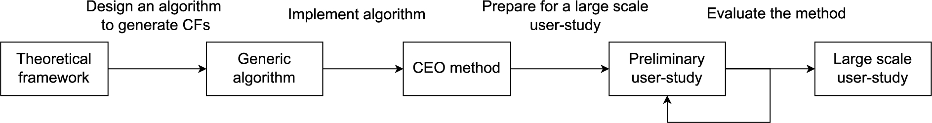
Fig. 1.

Flowchart of our approach to generate counterfactuals for ontologies.

3.Approach

Our main objective is to generate counterfactual explanations for OWL ontologies to explain entailments or inconsistencies. To the best of our knowledge, this goal was never explored before. Our approach, presented in Fig. 1, follows the same steps as similar methods for machine learning. The design of a theoretical framework that connects the concepts of machine learning to OWL ontologies is key to being able to adapt XAI methods to OWL ontologies. Once this framework is introduced, we can devise a generic algorithm to generate counterfactuals that is similar to the one applied in machine learning. Nevertheless, some challenges arise due to the fundamental differences between machine learning and ontologies. These challenges are studied and addressed in order to design the resulting CEO method. Finally, we intend to evaluate this method by conducting a rigorous large-scale user study. Due to the cost and complexity of such a study, we intend to run one or several preliminary user studies to detect issues in the study methodology and in the method that may hinder the quality of the large-scale study. A first iteration of such a preliminary study is presented and discussed in this paper.

Our overall approach replicates the approach followed by the XAI community to design counterfactuals for machine learning. An input and output are expected for the proposed method to function. These notions do not have an equivalent notion for ontologies. Hence, our approach will allow us to achieve the goal of generating counterfactuals for ontologies but may not fully take advantage of the mechanisms of ontologies.

The generic algorithm to generate counterfactuals follows the same mechanism as heuristic search methods i.e. explore the space of all possible counterfactuals and identify the best candidates according to a set of desired properties. The search space of candidate counterfactuals is defined and a heuristic is introduced to find the best candidates within this search space without exploring it entirely. The implementation of this algorithm is faced with several challenges such as the computation of the proximity metric and the design of an efficient heuristic. A proximity metric represents the difficulty of going from the original input to the counterfactual [20]. Determining such distance for entities of an ontology was already studied in the literature by using similarity metrics. We discuss the possible choices of such similarity metrics later in the paper. Regarding the design of a heuristic search, we represent the space of all possible counterfactuals (i.e. the search space) as a graph. Nodes are counterfactuals and edges represent elementary operations to go from one counterfactual to the other. This representation enables the use of graph edit distances to compute the different metrics.

The resulting CEO method is evaluated with two experiments. The first experiment uses objective metrics and particularly focuses on measuring the execution time required to generate the counterfactuals. The well-known Pizza ontology1 1 is employed as it fully exploits the possibilities of OWL ontologies. Moreover, its application domain does not require experts to understand and validate the explanations. The second experiment is a user study to assess the quality and relevance of the explanations. As discussed in Section 2, user studies are crucial to adequately evaluate the quality of an explanation method. However, conducting such a study is complex and expensive [6]. To circumvent this issue, our approach is to conduct several inexpensive small-scale studies to identify issues in the proposed method and the study methodology. A first preliminary user study on a musical instruments ontology is presented in this paper. The application domain of this ontology is chosen based on our easy and inexpensive access to domain experts. Due to its scale, the results cannot be generalized and may not be representative of the behavior of the method on other ontologies. Nevertheless, we expect that the results of these preliminary studies will provide enough feedback to detect problems in the explanations or methodology that are independent of the particular domain of application. This feedback will allow the preparation of a high-quality large-scale user study which will make the most of the resources allocated to it.

4.Theoretical framework to generate counterfactuals for OWL ontologies

We set to create counterfactual explanations for OWL ontologies based on the current works in machine learning. The first task is to map the definitions of desired properties seen in Section 2.2 to the OWL ontologies domain. This mapping paves the way for our method described in Section 5. We use the OWL2 language as defined in [33] and its mapping to RDF Graphs given in [34]. For ease of reading, an ontology’s class defined in its TBox is written as Class. Any term defined in the OWL2 specification [33], the RDF specification [32] or the mapping from OWL2 to RDF [34] is written in italics.

First, the problem is reformulated, then the desired properties of a counterfactual, i.e. validity, proximity, sparsity, feasibility, and diversity, are defined for OWL ontologies.

4.1.Problem formulation

The CF problem in machine learning is the following. Given a model f and an input vector x, a counterfactual of x is a vector xˆ such as f(x)≠f(xˆ). Specifically, only the supervised classification problem is studied. Let Co be the original class predicted by f(x) and Cd be the desired modified outcome. In the loan application example described in Section 2.2, Co corresponds to the class Denied, and the desired outcome Cd is the class Approved. The classifier f becomes an OWL ontology O. Indeed, both the classifier’s trained parameters and the ontology contain knowledge under different forms.

Any input vector can be seen as an individual defined in the ontology’s ABox. Each feature of this input vector corresponds to an assertion. Therefore, the input vector corresponds to the set of assertions that share the same sourceIndividual. With the RDF Graphs representation, each assertion is a triple of the form (subject−predicate−object) [32]. Since every assertion of this set shares the same sourceIndividual, these assertions can be rewritten as RDF triples where their Subject is the same. Finally, this enables the representation of this set of assertions as a star graph, where nodes are the objects of these assertions and edges are their predicates. The center node is the shared individual. This RDF graph corresponds to the input vector x. In the remainder of this paper, this type of graph is named an Individual Knowledge Graph or IKG. Let I be an IKG, the individual at the center of this IKG is noted Ic. Assertion, RDF triple, or triple will also be used interchangeably from now on. Let I be an IKG containing the triple (Ic−rdf:type−Co). The IKG Iˆ is a counterfactual of the IKG I if it contains the triple (Iˆc−rdf:type−Cd) and not the triple (Iˆc−rdf:type−Co).

Fig. 2.

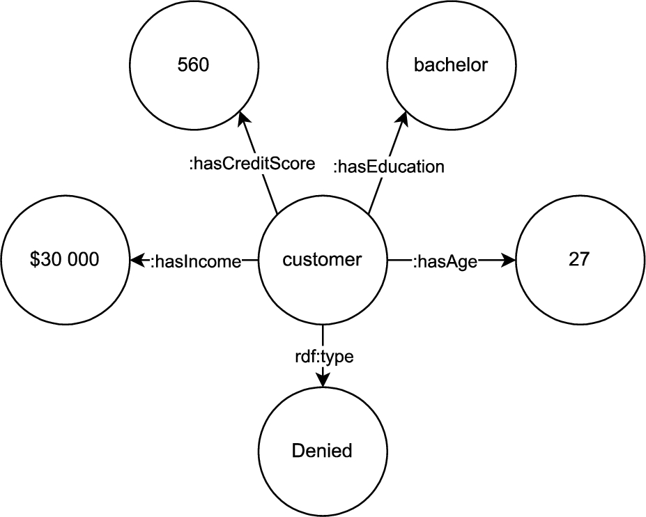
An IKG representing a customer classified as Denied with Income=$30K, CreditScore=560, Education=bachelor and Age=27.

A graphical representation of an IKG is proposed in Fig. 2. The subject of this IKG is the customer of the bank. Every assertion in the ontology that has this particular customer as subject is represented in the IKG, in the form of RDF triples.

4.2.Properties definition

Now that the definition of a counterfactual for an OWL ontology has been given, the different properties seen in Section 2.2 can be applied. In this section, I is the original IKG of class Co, that is to say I contains the triple (Ic−rdf:type−Co). It is assumed that if an IKG contains the triple (Ic−rdf:type−C), then it also contains every triple where the object is a parent of C. Equivalently, if an IKG does not contain the triple (Ic−rdf:type−C), then it does not contain any triple where the object is a subclass of C.

Validity	Based on the definition for machine learning, a counterfactual is valid if the outcome is the one expected. Therefore, we consider a counterfactual Iˆ valid if: – It contains the triple (Iˆc−rdf:type−Cd). – It does not contain the triple (Iˆc−rdf:type−Co). – The ontology is consistent after adding the IKG Iˆ to its ABox.
Proximity	Proximity is a measure of the distance between the original input and its counterfactual. In the literature, the problem of measuring the distance between two semantic entities has already been explored. Similarity functions are preferred to distances because they do not need to verify the triangle inequality. Similarities based on description logics are discussed in [21]. Euzenat et al. [9] present the OLA similarity which first encodes an ontology as a labeled graph; the similarity between two nodes of this graph depends on the similarity of the terms (labels, names…), the similarity of the neighbors and the similarity of other local descriptive features. Hu et al. [13] introduce the notion of signature vectors. The idea is to decompose a concept C into a set of primitive concepts and attribute a weight to each of these primitive concepts based on their number of occurrences in C. This concept C can now be represented as a vector where each feature is a primitive concept and the value of the feature is the importance of this primitive concept for C. Computing the similarity between two concepts is equivalent to computing the similarity between their signature vectors. The principal challenge of this method is to define those primitive concepts. For each ontology, primitive concepts must be defined which can be an arduous task for large ontologies. Finally, S. Ontañón [21] discusses the “edge counting” distance, first introduced by Rada et al. [23]. This distance is applicable to taxonomies and hierarchies. The taxonomy is seen as a tree where the parent relation defines the edge between the elements in the tree. The distance is simply the number of edges that must be traversed to go from one element of the tree to another. Overall, there exists a large choice of semantic similarity metrics, each adapted to specific use cases.
Sparsity	Sparsity is the number of features modified on the original input to get the counterfactual. For IKGs, the definition remains the same, it is the number of assertions of the original IKG that have been modified to get the CF.
Feasibility	Feasibility or plausibility is the measure of how realistic and achievable a counterfactual is. Because ontologies use domain knowledge, an unrealistic counterfactual should not be consistent with the ontology. Thus the consistency of the ontology reflects the plausibility of the counterfactual. Nevertheless, the issue of actionability persists. A CF is not feasible if it modifies non-actionable features. That is why we propose to flag some predicates as non-actionable in the ontology. For instance, a triple (Ic−:hasRace−Caucasian) should not be modified since race is a protected feature. Any triple with this predicate is not actionable, therefore, the predicate definition should reflect this non-actionability. One way to do so that is used in the CEO method is to consider non-actionable predicates as subclasses of an abstract class `NonActionable`
Diversity	Diversity being the distance between two counterfactuals, the similarity function used for proximity can be applied to two counterfactuals to compute the diversity.

5.Counterfactual explanations for OWL ontologies

The CEO method takes an IKG I as input and seeks a set of valid counterfactuals, as defined in Section 4. In the current state of our method, only ClassAssertions and ObjectPropertyAssertions are observed. A new set of ClassAssertions is decided by the user. The set of ClassAssertions of I is then replaced by the user-defined set. The new IKG resulting from this replacement is called Iˆ and is considered the closest counterfactual from I. However, it is likely that these changes render the ontology inconsistent. The method seeks appropriate modifications of the ObjectPropertyAssertions in Iˆ to make the ontology consistent with the changes in ClassAssertion. The CEO method is a black-box method according to the definition given for OWL explainability methods in Section 2.1. Indeed, it uses the reasoner as an oracle to check whether the addition of an IKG renders the ontology inconsistent.

A major difference between supervised classification and OWL ontology reasoning is that supervised classification requires an input with a fixed set of features. An OWL ontology reasoner does not impose a specific set of assertions to make inferences. To do so, those reasoners use the open-world assumption which considers that non-specified assertions are unknown. Thus, the open-world assumption should be taken into account when generating counterfactuals for OWL ontologies. Removing or adding assertions may provide additional information to the user and should be included in the method. Different sets of modifications, insertions, and removals are found by the method, sorted based on a set of metrics and proposed to the user as counterfactual explanations. Specifically, the generic algorithm to generate counterfactuals is decomposed into four parts:

1. Generate a set of candidate counterfactuals.
2. Remove nonvalid and non-feasible candidates.
3. Compute proximity and sparsity on the set of valid candidates.
4. Return the valid candidates to the user, sorted by proximity and sparsity.

The CEO method which implements each step is further discussed in this section. First, a simplification is made about the subject of every triple. In the definition of an IKG in Section 4, the subject of any triple in an IKG I is an individual noted Ic. It can be argued that for any counterfactual Iˆ of I, Ic=Icˆ. Indeed, this individual is the only constant thing between the original IKG and its counterfactual. For instance, let Ic be the bank’s customer from the loan application example in Section 2.2. The counterfactual provides possible modifications of assertions to obtain the loan. The customer may be told to modify their Income or their Education but it does not make sense to modify the nature of the customer, i.e. the subject of these assertions. This is why, from now on, the individual subject of an IKG is considered constant and is noted Ic in every case.

5.1.Counterfactuals search space

Some counterfactual methods propose to define the search space for counterfactuals ([15,26]) and then compute the different metrics for the counterfactuals in this search space. In the case of OWL ontologies, this space can be represented as a directed graph.

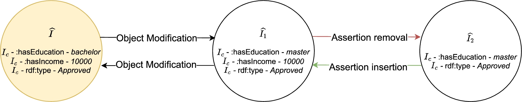
Let Ω=(V,E) be the graph representing the search space. V is a set of IKGs that are the nodes of this graph. E is the set of directed edges that link one IKG to another. Three elementary operations are defined on an IKG:

Object modification	This operation consists in modifying the ClassAssertions of an object in a triple.
Assertion removal	This operation consists in removing an assertion from an IKG.
Assertion insertion	This operation consists in adding an assertion to an IKG.

Two IKGs are connected in the graph if and only if a single elementary operation is needed to go from one IKG to the other. For instance, let Iˆ={(Ic−:hasEducation−bachelor),(Ic−:hasIncome−10000)} and I1ˆ={(Ic−:hasEducation−master),(Ic−:hasIncome−10000)}. This graph is represented in Fig. 3. Iˆ and I1ˆ are connected in Ω because a single object modification needs to be applied to go from Iˆ to Iˆ1, namely changing bachelor to master. Let Iˆ2={(Ic−:hasEducation−master)}. In this case, Iˆ and I2ˆ are not connected because more than one elementary operation should be applied. But I1ˆ and I2ˆ are connected because only an assertion removal connects them, namely removing the :hasIncome assertion. Each elementary operation has an inverse operation as can be seen in Fig. 3. The inverse operation of object modification is itself. The inverse of assertion removal is assertion insertion and vice versa.

Fig. 3.

Representation of a subgraph of Ω.

5.2.Exploring the search space

The graph Ω contains all possible IKGs, making it complex to compute. Moreover, only a fraction of the IKGs in this graph are valid. Therefore, the graph can be generated in an optimized manner, by avoiding non-valid IKGs. As a reminder, a counterfactual of the IKG I is an IKG that contains the triple (Ic−rdf:type−Cd) and not the triple (Ic−rdf:type−Co) where Co is the class of the original IKG and Cd is the desired class of the counterfactuals. Let CA(I) be the set of ClassAssertions of the IKG I, OA(I) the set of ObjectPropertyAssertions of I and DA(I) the set of DataPropertyAssertions of I. The simplest counterfactual of an IKG I is Iˆ and is defined in Equation (6). It is unlikely that this counterfactual is consistent and therefore valid, but it is the closest to the original IKG I. Thus, this IKG is an ideal starting point to explore the graph Ω.

(6)CA(Iˆ)=CA(I)∖{(Ic−rdf:type−Co)}∪{(Ic−rdf:type−Cd)}OA(Iˆ)=OA(I)DA(Iˆ)=DA(I)

Algorithm 1

Algorithm to generate a relevant sub-graph of Ω

Algorithm 1 is proposed to generate Ω. The graph is created with Iˆ as the starting node. Nodes that are connected with Iˆ by assertion removal operation are explored and added to Ω until consistent ones are found, with the findRemovalNeighbors function. Once these consistent nodes are known, the generateAncestors and generateDescendants functions are invoked on every explored node. These functions generate new nodes and edges by inserting back the removed assertions and modifying the class of their objects. The class of the objects must remain within the range of the predicate of the assertions.

This algorithm guarantees to obtain at least a consistent CF. In the worst case, this CF is an IKG with no assertion. Intuitively, the algorithm searches for faulty assertions that provoke inconsistencies, by removing them. When a consistent IKG is found, this means that every faulty assertion has been removed. These faulty assertions are added back one by one with modifications on their objects to fix the inconsistency.

However, the number of candidate counterfactuals explored by Algorithm 1 in the worst case is exponential with the number of assertions in the original IKG. Therefore, this algorithm does not scale up well with large ontologies. Moreover, a reasoner is called for every node generated. When the number of entities in the ontology increases, the reasoning time and the number of candidate counterfactuals to explore also increase.

5.3.Computing metrics in the graph

This graph representation enables the use of a graph edit distance to measure proximity.

(7)GED(I1,I2)=min(e1,…,ek)∈P(I1,I2)∑i=1kc(ei)

The graph edit distance written as GED(I1,I2) is defined in Equation (7), where P(I1,I2) is the set of edit paths transforming I1 to I2 and c(e) is the cost of each elementary operation. The cost for each elementary operation must be defined. Let cm(e) be the cost for a class modification operation, cr(e) for assertion removal operation and ci(e) for assertion insertion. We argue that for a given assertion, the cost of removing this assertion should be greater than modifying it. Likewise, inserting this assertion should cost more than removing the given assertion. This choice is justified by the feasibility and comprehensibility of an operation. The original IKG directly represents the real world therefore it is feasible.

Modifying the original assertions lowers the feasibility as it strays further away from the real-world example. This decrease is proportional to the similarity of the modified assertion with the original one. It represents the effort that the user has to make to go from their starting point to the new class. Removing an assertion removes any information about the changes to achieve, the user loses information about what and how they should change concerning the assertion. Finally, inserting an assertion requires the user to achieve something that was absent from their starting point, which may lead to unfeasible or incomprehensible requests. For instance, the assertion (customer−:hasEducation−bachelor) is studied. Modifying the class of the object means that the customer should change its education level, the greater the change is, the less feasible it is. Removing this assertion removes information about the change they must achieve. They should perhaps lose their degree, which is not feasible, or change their degree in an unknown way. Removing an assertion leads to incomprehensible but not necessarily unfeasible changes. Finally, inserting an education level is difficult to comprehend. The education level was missing from the original input, adding it may not make sense depending on the reason for its original absence. Moreover, achieving this change might not be feasible based on the customer status.

Arguably, adding an insertion should be costlier than removing an assertion, which should be costlier than modifying an assertion. The following costs are proposed:

Class modification	The cost is the similarity measure between the original class and the modified class.
Assertion removal	The cost is greater than the cost of any class modification on this assertion.
Assertion insertion	The cost is greater than the cost of removing this assertion.

Equation (8) is the proposed cost function, where sim is a similarity measure for two assertions and A is the space of all possible assertions.

(8)c(e)=sim(a1,a2)if e is a class modification operation from assertions a1 to a2maxa∈Asim(a1,a)+1if e is an assertion removal operationwhere a1 is the studied assertion.maxa∈Asim(a1,a)+2if e is an assertion insertion operationwhere a1 is the studied assertion.

Proximity is the similarity between any counterfactual and the original input I. Since the GED only allows to compute similarity between nodes in the graph, the original input is replaced by Iˆ which is considered the closest counterfactual from I. Thus, proximity of a counterfactual Iiˆ is GED(Iˆ,Iiˆ), with the cost function defined in Equation (8).

It is also possible to compute sparsity in the same manner, with a different cost function. Indeed, an edge of the graph is an elementary operation on one assertion. Therefore, the shortest path between two IKGs contains one edge per modified assertion. The length of this path is equal to the number of modified assertions. Thus, the GED with ∀e,c(e)=1 as cost function is a measure of sparsity. Finally, a similarity measure should be defined to compare two objects of an assertion.

5.4.Assertions similarity

In Section 4.1, an IKG is defined as a set of assertions sharing the same sourceIndividual. The proximity metric for machine learning computes the distance between each feature and then aggregates these distances to get the proximity. The same idea can be applied to an IKG, by comparing assertions together. This raises the issue of comparing two assertions. The methodology of proximity for machine learning could be applied, i.e. decompose the triple, measure the distance between each element of the triple, and aggregate these distances. However, in the case of counterfactuals, we will show that the distance between triples can be simplified into the distance between the objects.

Problem simplification The predicate of an RDF triple represents the nature of the relation between the subject and the object. Can a distance between two predicates be defined and is it sensible to compare two triples of different predicates? For instance, what is the distance between the predicates rdf:type and :hasAge? In machine learning, only the same features were compared. Hence, only similarity between triples with the same predicate is defined.

In the introduction of Section 5, it was argued that the sourceIndividual remains the same for counterfactuals. Likewise, only triples with the same predicate should be compared. Therefore, measuring the similarity between two triples can be simplified into measuring the similarity between the respective objects of these triples. The subject of any triple in an IKG is an individual. According to the mapping of OWL2 to RDF [34], assertions that have an individual as subject can be of the following types: SameIndividual, DifferentIndividual, ClassAssertion, ObjectPropertyAssertion and DataPropertyAssertion. Therefore, the possible types of objects are classes, individuals, and literals. The SameIndividual and DifferentIndividual assertions are not of interest for counterfactuals and are therefore removed from IKGs. DataPropertyAssertions have literals as objects. Similarity measures between literals such as strings or numbers already exist. ObjectPropertyAssertions require a similarity between two individuals. However, an ObjectProperty is defined with a Domain and a Range which are classes. The individual must belong to this Range, thus it must have a ClassAssertion. That is why the same similarity will be used for classes and individuals.

Edge-counting similarity The edge-counting similarity measure proposed by Rada et al. [23] is a good choice for computing similarities between classes because of its simplicity to understand and visualize. This similarity measure is based on hierarchical is-a relations. In OWL ontologies, such hierarchy is obtained with the SubClassOf relation. A hierarchy tree is created where the edges are the SubClassOf relation and the nodes are classes. The similarity between two classes is the length of the shortest path from one class to the other in this tree.

Concerning individuals, three cases are possible:

– If the individual is not subject of any ClassAssertion, then the class used is owl:Thing which is the root of the tree.
– If the individual is subject of a single ClassAssertion, this class is used to measure the similarity with another individual.
– If the individual is subject of multiple ClassAssertions, then the similarity between each class is calculated and the smallest one is kept.

This particular similarity measure is used to compute the weight of the edges associated to class modification operations for the graph edit distance described in Section 5.3.

In conclusion, the CEO method takes an IKG as input and a set of desired classes given by the user. A subgraph of all possible counterfactuals is generated in a way that guarantees at least one valid counterfactual. Invalid and unfeasible counterfactuals are removed from the set of candidate counterfactuals. Specifically, non-actionable assertions are assertions that have an ObjectProperty which is a SubClassOf an abstract property named NonActionable. If an assertion with this predicate is modified, the CF is considered unfeasible. Then, the proximity and sparsity are computed for every valid and feasible counterfactual. Finally, the counterfactuals are sorted by proximity and sparsity and displayed to the user. Since proximity and sparsity have the same order of magnitude, they are added together to get the ranking of counterfactuals.

6.Experiments

In order to validate the CEO method and identify points of improvement, two experiments are conducted. The first experiment focuses on measuring the execution time of the CEO method and whether it returns the expected results. The second experiment is a small-scale user study designed to verify the relevance and comprehensibility of the explanations. This user study is a preliminary to a larger user study, the intent is to detect issues in the method and the survey methodology that would hinder a larger scale and expensive user study.

6.1.Experiment on execution time

This first experiment is focused on studying the execution time of the CEO method. Four cases are generated with the Pizza ontology.2 2 Each case represents a pizza of a specific class (e.g. vegetarian pizza) paired with assertions such as the toppings or the base. The goal is to understand how the CEO method behaves with a different number of faulty and correct assertions. Specifically, we monitor the running time of each step of the heuristic in relation to the number of candidate counterfactuals explored. Moreover, we declare some counterfactuals that we expect e.g. change meat topping to vegetable topping to obtain a vegetarian pizza. The rank of these expected counterfactuals is monitored to verify that they are generated by the method and are among the counterfactuals with the lowest proximity.

6.1.1.Test cases and results

Let Co={MeatyPizza}, Cf={VegetarianPizza}, Af a set of faulty assertions that will produce inconsistencies with Cf and Ac a set of correct assertions that will not lead to inconsistencies. The CEO method is applied to generate a set of valid counterfactuals, with I=Co∪Af∪Ac as the input IKG, Co as the set of classes to change and Cf as the foil (i.e. desired) set of classes.

Case 1: One faulty assertion The first case is an individual that has only one faulty assertion.

Ac=∅Af={(i−:hasTopping−chickenTopping)}

We expect the counterfactuals to modify chickenTopping into vegetableTopping or cheeseTopping. The CEO method generated 41 valid counterfactuals out of 52 explored candidates. The proximity of the expected results was tied with 5 other counterfactuals and was the second smallest proximity. The counterfactual with the smallest proximity modifies chickenTopping to pizzaTopping which could represent any topping. The second smallest proximity corresponds to a modification of chickenTopping to direct subclasses of PizzaTopping e.g. CheeseTopping, FruitTopping or VegetableTopping. The counterfactual with the highest proximity is the only one that deletes the assertion.

Case 2: One faulty and one correct assertion This second example adds a correct assertion to the previous case.

Ac={(i−:hasTopping−mozzarellaTopping)}Af={(i−:hasTopping−chickenTopping)}

We expect the counterfactuals to leave the assertion in Ac untouched and to modify chickenTopping into vegetableTopping or cheeseTopping. The CEO method generated 348 valid counterfactuals out of 911 explored candidates. We note that the amount of explored and valid counterfactuals drastically increased compared to the previous case. The ranking is similar to the last case for the first 41 counterfactuals, meaning that the expected counterfactuals ended up at the same rank with the same proximity. The CEO method tested almost every combination of pairs of toppings resulting in this increase in the number of counterfactuals generated.

Case 3: Two faulty assertions To assess the impact of faulty assertions, we propose an example that also has two assertions similar to the previous one, but both assertions are now faulty. Therefore, we set Ac and Af as follows.

Ac=∅Af={(i−:hasTopping−chickenTopping),(i−:hasTopping−hamTopping)}

We expect the counterfactuals to change both assertions into any combination of vegetableTopping and cheeseTopping. The CEO method generated 317 valid counterfactuals out of 1160 explored candidates. Compared to the previous case, more counterfactuals were explored but fewer were valid. It can be explained by the increased difficulty to get the individual consistent since both assertions are faulty. The number of explored counterfactuals did not change significantly because the assertions are of the same nature resulting in the same combinations to explore. The first 40 counterfactuals in the ranking have modified one topping into the abstract class pizzaTopping while exploring every valid topping on the other assertion. Thus, our expected counterfactuals are not in these 40 counterfactuals. The rest of the assertions are similar to the last case, with every valid combination of two toppings.

Case 4: One faulty topping, one faulty base We propose an additional test case that differs from the other in the nature of the assertions. The aim is to test the influence of the predicate on the number of counterfactuals explored.

Cf={VegetarianPizza,RealItalianPizza}Ac=∅Af={(i−:hasBase−deepPanBase),(i−:hasTopping−chickenTopping)}

The RealItalianPizza class imposes that the base is of class ThinAndCrispyBase. The number of counterfactuals explored is proportional to the number of classes in the range of a predicate. The predicate :hasBase has only three classes in its range. Therefore, a decrease in the number of explored counterfactuals should be observed. The expected counterfactual is the modification of deepPanBase to thinAndCrispyBase and the modification of chickenTopping to vegetableTopping.

The CEO method generated 123 valid counterfactuals out of 208 nodes explored which validates our expectations. The 10 best-ranked counterfactuals modify the topping with different classes while always changing the base from deepPanBase to the abstract pizzaBase, except for the tenth counterfactual which changes the base to the expected thinAndCrispyBase. Then, every possible combination of base and topping is generated. Abstract classes (e.g. PizzaTopping or PizzaBase) are attributed a lower proximity which favors them in the ranking. The expected counterfactual is found by the method but ranked at the 42nd position.

Finally, we note that running these examples allowed us to identify design issues in the Pizza ontology.3 3 These issues are intentional as the initial goal of the Pizza ontology is to act as a tutorial that highlights typical design errors that can be made when building an ontology. Nevertheless, the CEO method showed its ability to detect such issues.

6.1.2.Analysis

The experiments showed that the expected counterfactuals are always generated but not always well-ranked. The computation of proximity favors these abstract classes as they systematically have the lowest proximity and thus highest rankings. This is due to the computation of proximity which uses the edge-counting dissimilarity measure. This dissimilarity penalizes classes that have the same level of abstraction. For instance, the dissimilarity between the classes ParmezanTopping and MozzarellaTopping is 2. Yet, they are both direct subclasses of CheeseTopping which should make them highly similar. The edge-counting dissimilarity favors parent classes, the dissimilarity between CheeseTopping and any direct subclass is always 1. As a result, abstract classes lead to low proximity.

Consequently, the top counterfactual is always too abstract to the point that it does not provide any relevant information. In the studied cases, the top counterfactual always modified the faulty assertions to pizzaTopping, meaning that the meat should be replaced by anything. Users who are not experts in ontologies or who do not know the functioning of the CEO method may be confused by this counterfactual. Giving the information that meaty toppings are problematic and should be replaced with any topping that isn’t meaty may be more valuable to the user.

Fig. 4.

Bar plot of the detailed execution time for each example.

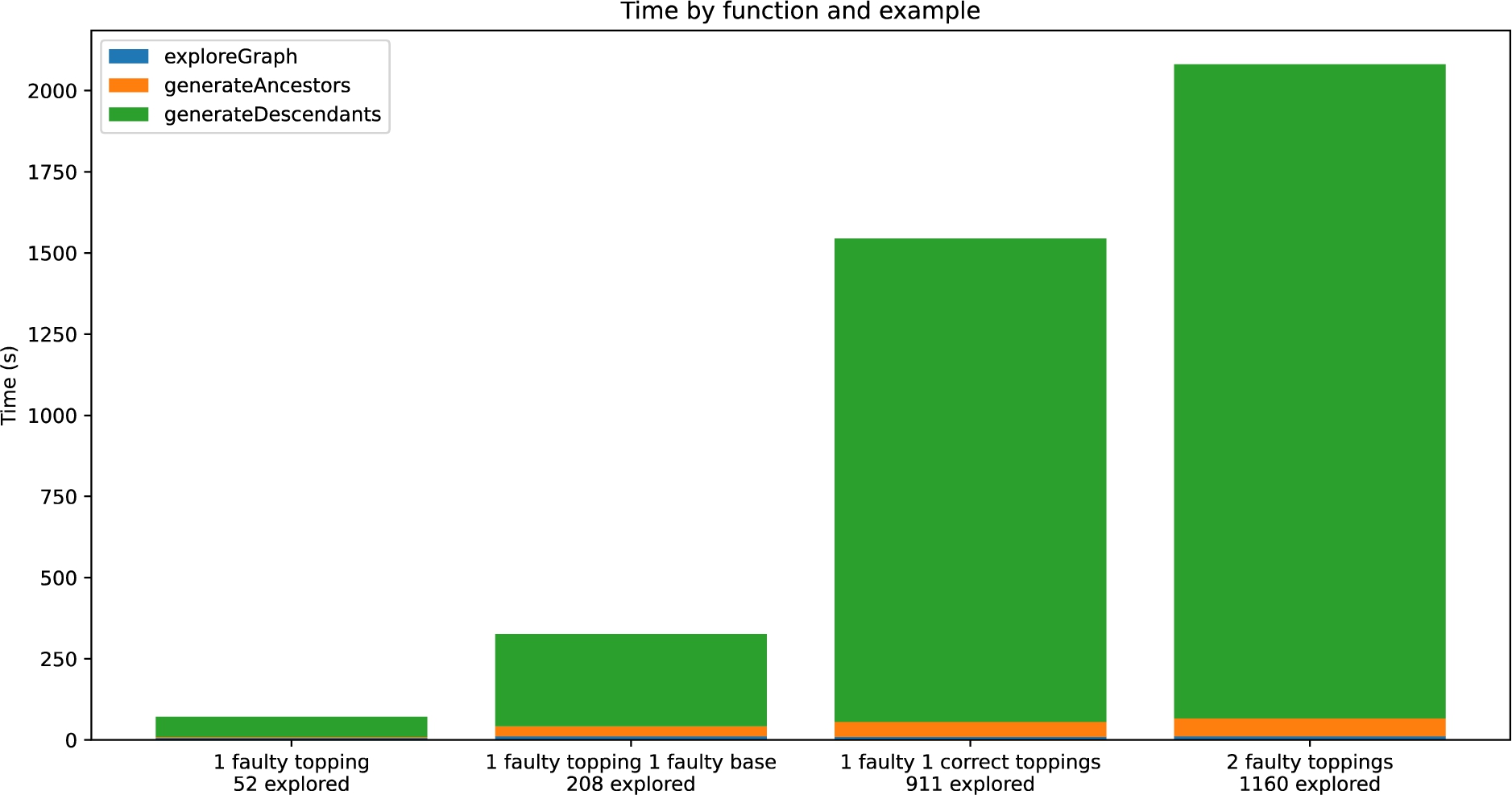
The execution time observed in these test cases is not satisfactory. Figure 4 demonstrates that the last step of the CEO method represents approximately 90% of the total execution time. The execution time is tightly linked to the number of explored nodes. The heuristic seeks every consistent combination of assertion modifications. The number of possible modifications for one assertion is dictated by the number of defined classes within the range of the assertion’s predicate. In the Appendix, we pose the formula to calculate the size of the search space based on the number of classes within the range of each assertion’s predicate. Cases 3 and 4 illustrate the consequence of the size of the search space on the number of explored nodes The range of the predicate :hasBase contains 3 classes, while the range of :hasTopping has 52 classes. The size of the search space for case 3 is 2809 while for case 4 it has a size of 212. The difference in search space explains the difference in scale in the execution time. More than 90% of this time is spent by the logical reasoner4 4 which is called for every explored counterfactual.

Overall, the CEO method generates valid counterfactuals, including the expected ones. Nevertheless, it faces the same problem as heuristic-based machine learning counterfactual methods i.e. a high execution time due to large search spaces. In its current state, the CEO method does not take diversity into account when exploring the search space. Maximizing diversity might be a way to decrease the number of explored counterfactuals without hindering the quality of the proposed counterfactuals. Regarding the execution time, further investigations to reduce it should be conducted. A possible direction is to explore ways to reduce the number of calls to the logical reasoner and optimize the execution time of the logical reasoner. The heuristic may also be tuned to limit the number of counterfactuals explored. For instance, the user may choose to ignore certain classes to decrease the size of the search space e.g. ignore leaf classes such as ArtichokeTopping or CaperTopping to focus on their parent class VegetableTopping.

6.2.Preliminary user study

The evaluation of the explanations generated by the CEO method requires a user study as the quality of an explanation is mostly subjective. We discussed in Section 3 that a large-scale user study is expensive and complex to conduct. Therefore, the quality of the survey and the method that is evaluated should be flawless to avoid wasting resources. In this section, we conduct a preliminary user study that mimics this large-scale user study but with reduced expenses and complexity. The intent is to discover potential issues with the method and survey methodology. The goal of the user study is to verify the relevance and comprehensibility of the explanations. In this preliminary study, the experimental context described in [5] is used.5 5 This choice is motivated by privileged access to experts in this domain.

An ontology is created, based on a simple hierarchy of musical instruments families. There are 17 classes that each represent a musical instrument. 5 object properties are used in the class definition of these instruments: the texture, the mechanism, the type of mouthpiece for wind instruments, the shape, and the presence of visible strings. Several convolutional neural networks with the ResNet50 architecture, pretrained on the ImageNet dataset have been finetuned on 4000 pictures of musical instruments. One of those models detects the type of instrument while the others detect each object property defined in the ontology of musical instruments. The results of these models are added to the ontology as an IKG. If the ontology is inconsistent after these additions, that means that the instrument detected is not consistent with the properties detected. The study follows up on this idea and proposes counterfactual explanations to render the prediction consistent. For instance, a harpsichord is detected as well as pedals and a wooden texture. This is not consistent with the ontology because a harpsichord does not have pedals. The goal of the CEO method is to propose modifications for these inconsistent assertions so that the user understands which properties were wrong and how to change them.

Fig. 5.

Description and the first four explanations of the first case of the survey.

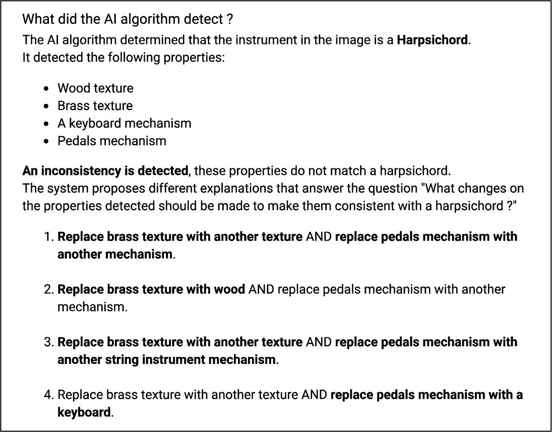
Fig. 6.

Input image of the first case of the survey.

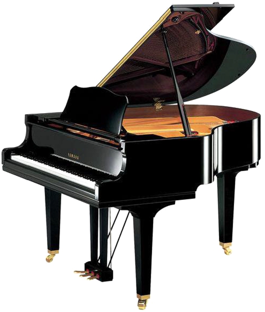
At the beginning of the survey, the users are first presented a description of this system, what its goal is, and how it works. Then, an image is presented with the output of the machine learning models. Figure 5 shows the description of the output of the models for the first case of the survey and the explanations, with Fig. 6 as the input image. It is explained that the results are not consistent with expert knowledge and finally, a question is formulated: “What changes on the properties detected should be made so that the ontology is consistent?”. A set of valid and feasible counterfactuals is generated and sorted by proximity and sparsity. The first ten counterfactuals are proposed to the user, hiding the rest of the generated set. A counterfactual is presented as a text telling the user which changes to make in no particular order. An example of a counterfactual given to a user is the following: “Replace brass metal texture with wood AND remove pedals mechanism”.

Then, the user answers two questions:

1. Which explanation did the user prefer?
2. Which explanations seemed relevant to the user?

These questions enable the evaluation of the quality of explanations and the quality of the proximity metric. Ideally, the preferred explanations are within the first explanations because they are sorted by proximity and sparsity. The last question permits to plot the ROC curve (Receiver Operating Characteristics) which represents the number of relevant explanations on the y-axis and the amount of non-relevant explanations on the x-axis. The Area Under the Curve (AUC) for the ROC curve is used in information retrieval to measure the capacity of a system to rank the relevance of documents [3]. In this study, the AUC ROC is a measure of the quality of the ranking of explanations, therefore is a proxy measure of the quality of the proximity and sparsity metrics.

The user study was conducted on a sample of six domain experts, i.e. experienced musicians. Nine different examples were presented. To identify issues with the explanations and methodology, a discussion took place with each expert after the survey in order to get their feedback.

6.2.1.Results

Results are combined in Tables 1 and 2. Table 1 shows the rank of the preferred explanations and the percentage of experts that chose them, the percentage of relevant explanations, and finally the average AUC ROC for each case. The AUC ROC is calculated based on the answer of each expert, and then the average of these scores is displayed in the table. Table 2 shows key statistics for each rank of explanation. A consensus is reached when 50% or more agree on the preferred explanation.

Table 1

Results of the user study for each case presented to six domain experts

Case	Preferred explanations (% who chose it)	% of relevant explanations	Average AUC ROC
1	2nd (16.7%), 3rd (16.7%), 7th (50%), 8th (16.7%)	70%	0.77
2	5th (16.7%), 10th (83.3%)	90%	0.55
3	1st (33.3%), 3rd (50%), none (16.7%)	22%	0.93
4	6th (33.3%), 7th (16.7%), 8th (33.3%), 10th (16.7%)	80%	0.55
5	2nd (83.3%), none (16.7%)	20%	0.96
6	3rd (16.7%), 8th (16.7%), 9th (50%), none (16.7%)	50%	0.76
7	1st (16.7%), 3rd (50%), 9th (16.7%), none (16.7%)	40%	0.87
8	7th (33.3%), 8th (66.7%)	80%	0.65
9	1st (16.7%), 3rd (66.7%), 9th (16.7%)	20%	0.78

Table 2

Results of the user study for each rank of explanation

Explanation ranking	1st	2nd	3rd	4th	5th	6th	7th	8th	9th	10th
Proportion of relevance	9/9 (100%)	7/9 (78%)	7/9 (78%)	4/9 (44%)	3/9 (33%)	4/9 (44%)	4/9 (44%)	4/9 (44%)	3/9 (33%)	2/9 (22%)
Number of consensus	0/9 (0%)	1/9 (11%)	3/9 (33%)	0/9 (0%)	0/9 (0%)	0/9 (0%)	1/9 (11%)	1/9 (11%)	1/9 (11%)	1/9 (11%)
Occurrences of preference	4	6	12	0	1	2	6	8	5	6

The first observation from Table 1 is that the quality of the explanations is highly dependent on the case. Indeed, the amount of relevant explanations varies from 20% up to 90%. Cases 3, 5, and 9 are the only ones to include an assertion about the shape of the instrument. Experts have identified a flaw in the ontology concerning the shape property based on the generated explanations. The poor relevance of these cases can therefore be attributed to this error. Table 3 is the same as Table 2 without cases 3, 5, and 9 which may bias the analysis of preferences since only the first three explanations were relevant.

Table 3

Results of the user study for each rank of explanation after removing cases 3, 5, and 9

Explanation ranking	1st	2nd	3rd	4th	5th	6th	7th	8th	9th	10th
Proportion of relevance	6/6 (100%)	6/6 (100%)	5/6 (83%)	4/6 (67%)	3/6 (50%)	4/6 (67%)	4/6 (67%)	4/6 (67%)	3/6 (50%)	2/6 (33%)
Number of consensus	0/6 (0%)	0/6 (0%)	1/6 (16.7%)	0/6 (0%)	0/6 (0%)	0/6 (0%)	1/6 (16.7%)	1/6 (16.7%)	1/6 (16.7%)	1/6 (16.7%)
Occurrences of preference	1	1	5	0	1	2	6	8	4	6

The AUC ROC is always greater than 0.5 which indicates that the relevant explanations are not packed at the bottom of the ranking. Table 3 also shows that the proposed explanations are relevant in more than 50% of cases, except for the tenth explanation. However, the top explanations are not preferred by the experts. Because of the small sample size, the occurrences of preference for each rank are also displayed in Tables 2 and 3. This measure is the number of times it was preferred by any expert in every case. It does not take into account when experts did not have a preferred explanation, which happened in cases 3, 5, 6, and 7. The last four explanations stand out as being the most preferred, by cumulating a total of 24 preferences over 34 votes.

Concerning the content of the explanations, the first explanations are the most abstract. They successfully identify the faulty assertions but give a generic change, such as “replace wood by another texture” or “replace the strings by another mechanism”. Preferred explanations are rarely in the top ranks because experts sought more specific changes that have the same level of abstraction as the original assertion. The other explanations are grouped by possible modifications on one assertion. For instance, in case 1, the 3rd to 6th explanations only explore modifications to the mechanism without modifying the other assertions. Finally, removal operations are usually positioned at the bottom of the ranking because of the way the cost of these operations is computed. However, as Table 3 demonstrates, experts prefer explanations at the bottom of the ranking.

Overall, the experts complained that the survey necessitated an important cognitive effort and struggled to interpret the explanations. They argued that the way of presenting the explanations was problematic and suggested an interactive interface rather than a simple text. Nevertheless, they unanimously found that counterfactual explanations are useful to understand a decision process. They also pointed out some issues in several explanations that come from flaws in the design of the ontology. Finally, they deplored the absence of assertion insertions that could have been highly relevant in some cases. For instance, wind instruments always have a mouthpiece. When a mouthpiece was not present in the original IKG, it was not present in the counterfactuals either. Experts expected the addition of a mouthpiece in these cases.

6.2.2.Analysis

The main point of this study was to assess whether the proposed explanations are relevant to identify issues in the CEO method that would alter the results of a larger-scale survey. Four cases had less than 50% relevant explanations and three among them were justified because of a faulty axiom in the ontology. Ontologies are designed with domain experts, therefore using the CEO method during the design phase can prove useful to detect errors. Indeed, the automatic exploration of candidate counterfactuals may create unexpected individuals that a human would not have tested. However, the current exploration algorithm is computationally costly since the number of counterfactuals generated scales exponentially with the number of assertions in the original IKG.

The valid candidates generated and presented to the users are mostly relevant and the AUC ROC scores show good results. This would indicate that the proximity and sparsity metrics functioned as desired. However, the preferred explanations are mostly at the bottom of the ranking. This is an issue because experts complained that there were too many explanations for each case. If 5 explanations were retained instead of 10, the best explanations would have been missed. Likewise, the best explanations may not be present in the 10 explanations shown, since more than 10 valid candidates were generated for most cases. Therefore, the chosen proximity metric is not adequate to sort the explanations for this particular application.

Two problems with the proximity metric have been identified. First, explanations with the lowest proximity are the most abstract which is not what experts expect. They prefer to be shown classes that have the same depth as the original class. The similarity metric that compares two assertions should be modified to walk the hierarchical tree breadth-first instead of depth-first. Secondly, explanations with assertion removals are ranked at the bottom because of the design of the cost function. Yet it was shown that the bottom explanations are the most preferred. In some cases, the removal of an assertion was the expected explanation by the experts. The cost function for assertion removal should be modified to prevent relevant removals from being placed in the bottom explanations. These changes are relevant to this particular ontology. For other ontologies and applications, different similarities may be better suited. Finding a similarity suited for an application is a challenge that needs to be addressed to apply the CEO method.

Another issue of the current sorting system is that there are groups of counterfactuals that modify the same assertion. In Section 2.2, the notion of diversity was introduced. Adding diversity to the sorting system may alleviate this problem. Still, diversity is analogous to proximity and is exposed to the same issue which is the choice of a similarity metric. Furthermore, there is a risk that a high-quality explanation will not be displayed because it is too similar to a lower-quality explanation that got a better ranking. Before adding a diversity constraint, a satisfying proximity must be found. That is why diversity was not included in the current version of CEO.

As was pointed out by the experts, the lack of assertion insertion is problematic. Some explanations could have greatly benefited from such operations. The generation of the subgraph Ω must be reworked to include assertion insertions efficiently. Likewise, some counterfactuals are not explored and thus the best explanations may be missing from the set of valid and feasible counterfactuals. The impact of this issue is hard to measure since it is not possible to know if the best explanations have been explored. A cause of confusion for the experts was the meaning of removing an assertion. For them, removing an assertion meant that it is absent from the instrument. But with the open-world assumption, removing an assertion means that it is unknown, not missing. A way to render removal assertions more intuitive is to add NegativeObjectPropertyAssertions to the IKG when a removal operation is done. Thus removing an assertion will have the same meaning for the user and the OWL ontology. Similarly, the CEO method does not handle DataPropertyAssertions which may be needed in some applications such as the loan approval example described in Section 2.2.

To address the complexity of understanding the counterfactual explanations, their presentation should be reworked. An interactive interface that allows the user to see and visualize the explanations in the graph may decrease their cognitive effort to understand the explanations. Representing the graph of possible counterfactuals may also solve the problem of diversity, by visually identifying clusters of nodes that all modify the same assertion in different ways. This interface may also allow the user to modify key elements of the CEO method such as the similarity metric. A new user study should be conducted to verify this hypothesis.

6.3.Discussion

The conducted experiments demonstrated that the CEO method achieves our goal of generating counterfactuals for ontologies. The analysis of the execution time revealed that, in its current state, the execution time of the CEO method scales worse than linearly with the size of the search space. The size of the search space is linked to the size of the ontology; the method would not execute in a reasonable time for a large ontology. Other explanation methods for ontologies only run the logical reasoner a few times ([1,7]), whereas the CEO method calls it for every explored counterfactual. Hence, it is not yet adequate for debugging large ontologies. Still, this method is useful to explain the entailments to laypersons, unlike the existing explanation methods. Execution time is not a crucial factor in choosing explanation methods, which is why it was not a major focus of the CEO method.

The preliminary user study was conducted with a small sample size of six domain experts on a single ontology. Thus, the results may not be representative of the actual quality of the method, and a large user study on multiple ontologies with more subjects is required. Nevertheless, it uncovered several issues in the CEO method and the study methodology that would have impacted a larger user study. Namely, the proximity metric and ranking system that displays similar and abstract explanations. Similarly, the removal of an assertion is not intuitive and complicates the comprehension of the counterfactuals. These observations from the user study are aligned with our observations on the execution time experiment on a different ontology. Furthermore, the quantity and presentation of the explanations should be improved to facilitate their comprehension.

7.Conclusion

In this paper, counterfactual explanations for ontologies were studied, inspired by the literature on counterfactuals for machine learning. As a result, the Counterfactual Explanations for Ontologies (CEO) method was presented. It is divided into 4 steps. First, a graph of candidate counterfactuals is generated, then these counterfactuals are filtered to keep only the valid and feasible ones. Afterward, proximity and sparsity metrics are computed with a graph edit distance to finally present the explanations sorted based on these metrics. Each step is independent from one another. This renders the CEO method highly modular and adaptable. Choices for each step must be made based on the application. For instance, a tradeoff between computation time and the number of explanations generated must be made for the graph generation method. Likewise, concerning the proximity, an adapted similarity must be chosen. This modularity is both an advantage and a drawback. Indeed, the CEO method can be tailored to each user which is encouraged to improve explainability. However, it requires making informed choices for each step which makes it complex to implement. Two experiments on the CEO method were conducted. The first experiment focused on measuring execution time and ensuring that the expected counterfactuals are generated. The results demonstrated that the CEO method succeeds in identifying the expected counterfactuals. However, its execution time is high as the scaling is not linear with the size of the ontology. Although the process of generating explanations is not time-sensitive, the scalability of the method does not allow to apply it on large ontologies.

The second experiment is a preliminary user study intended to prepare for a larger-scale study. The domain of application of this experiment was motivated by our inexpensive and easy access to experts in this domain. The experiment was conducted on a musical instrument classification task, with the goal of verifying the relevance and quality of generated explanations. Six experts filled out a survey to assess the quality and relevance of explanations. The results of this method should not be used to compare CEO with different methods as the small sample size may skew the results. Likewise, the results should not be generalized to other ontologies. Nonetheless, this preliminary user study identified several problems regarding the CEO method and the study methodology that could have negatively impacted the results of a large-scale user study. Several points of improvement regarding the comprehensibility and quality of the explanations were identified. The proximity metric and the chosen similarity are not adequate for the tasks of the experiments. Moreover, some machine learning methods look for the most diverse explanations, which is not yet applied in the CEO method. It may help to find a variety of ideal explanations that are not too similar. Overall, the surveyed experts found the explanations overwhelming, due to the high number of presented explanations, the way they were presented, and the counter-intuitive nature of the removal operation.

Some choices in the implementation of the CEO method also lead to limitations. Insertion operations are not explored as they would significantly increase the size of the search space and consequently increase the execution time. Likewise, some types of assertions are not yet handled, namely DataPropertyAssertions and NegativeObjectPropertyAssertions. Handling these assertions may improve the compatibility of this method with a larger set of applications and improve the intuitiveness of the counterfactuals.

In future work, we plan to conduct a large-scale user study on multiple ontologies. Beforehand, the observed issues must be addressed. The addition of a diversity constraint will be explored to avoid groups of similar counterfactuals in the presented explanations. A positive side-effect of this addition will be to enable the decrease of the number of presented explanations without compromising on their relevance. In the meantime, other proximity metrics will be investigated to develop a library of proximity metrics that are suited for different tasks and audiences. Particularly, a variation of the edge-counting similarity that favors classes with the same depth will be investigated, as well as other classes of similarity metrics that were seen in the literature. The ability to handle new types of assertions will be added, especially NegativeObjectPropertyAssertions that may be used to address the intuitiveness problem of the removal operations. Regarding execution time, different heuristics to explore the graph more efficiently will be explored. Furthermore, in the presented CEO method, only hierarchical relations are exploited while the rest of the TBox is unused to explore the graph. Exploiting the TBox may reduce computation time without hindering the quality and diversity of explanations. Doing so may also facilitate the exploration of assertion insertions which is lacking in the current version.

Finally, other rounds of similar preliminary user studies will be required to ensure that the proposed improvements correctly address the issues. The large-scale user study will evaluate the quality and relevance of the explanations for multiple audiences e.g. ontologists, domain experts, or laypersons. Likewise, several tasks, application domains, and ontology sizes will be used to evaluate the ability of the CEO method to be compatible with most ontologies.

Notes

1 https://protege.stanford.edu/ontologies/pizza/pizza.owl

2 https://protege.stanford.edu/ontologies/pizza/pizza.owl

3 https://protege.stanford.edu/ontologies/pizza/pizza.owl

4 We used the Pellet reasoner for the experiments.

5 Code, ontology and evaluation data of this experiment are available at this link: https://github.com/matt-bellucci/CEO.

Appendices

Appendix

AppendixSize of the search space

The search space Ω is defined as the set containing every possible counterfactual of an individual. The current heuristic to explore this space does not insert new assertions to create counterfactuals. Therefore, the search space contains every combination of modification and deletion operations on the set of assertions of the original IKG. We note N the number of modifiable assertions of the original IKG i.e. every assertion except ClassAssertions. The total number of possible modifications for a single assertion is defined by the number of classes in the predicate’s range. Let ni be the number of classes in the predicate’s range for the i-th assertion.

Let us consider the case where N=2. The search space contains every possible modification of the two assertions, every possible modification on one assertion and the deletion of the other, and the deletion of both assertions.

(9)|Ω|=1︸Two deletions+n1+n2︸Deletion of one assertion+n1×n2︸No deletion

Equation (9) shows the size of the search space when N=2. There is only one combination when every assertion is deleted, n1 modifications when the second assertion is deleted, n2 modifications when the first assertion is deleted and n1×n2 modifications when both assertions are kept. We can apply the same reasoning for an undefined number of assertions.

(10)|Ω|=1︸Deletion of all N assertions+∑i=1Nni︸Deletion of N−1 assertions+∑(k1,k2)∈CN2nk1×nk2︸Deletion of N−2 assertions+⋯+∑(k1,…,kN−1)∈CNN−1∏j=1N−1nkj︸Deletion of 1 assertion+∏j=1Nnj︸No deletion

Equation (10) shows the intuitive formula of the search space. The first term is always 1 and corresponds to the deletion of all assertions. The second term corresponds to every combination for the deletion of every assertion but one. The third term calculates every combination of two assertions for every possible pair of assertions, where CNk represents the set of combinations of k assertions picked from a set of N assertions. For instance, C32 is the set of all possible unordered pairs picked from a set of three elements e.g. {(AB),(AC),(BC)}. In general, each term of Equation (10) corresponds to the number of possible counterfactuals for a given number of deleted assertions.

(11)|Ω|=∑i=0N∑(k1,…,ki)∈CNi∏j=1inkj

Equation (11) is the formula to calculate the size of the search space Ω. However, this formula is tricky to compute and we propose an alternative formula. We observe when rearranging Equation (10) that a pattern emerges as shown in Equation (12).

(12)|Ω|=1+n1+n2(1+n1)+n3(1+n1+n2(1+n1))+⋯

Let σ be a series defined as:

(13)σ(k)=1if k=01+n1if k=1nk∑i=1k−1σ(i)if k>1

Theorem A.1.

∀N⩾1∈N,|Ω|=∑i=1Nσ(i)

Proof.

We will prove this statement by induction.

Base case

For N=1, |Ω|=1+n1.

∑i=11σ(i)=σ(1)=1+n1=|Ω|

Inductive step

Suppose the theorem holds for all values of N up to some t, t⩾1. Let us verify the theorem for N=t+1.

∑i=1t+1σ(i)=σ(t+1)+∑i=1tσ(i)=nt+1∑i=1tσ(i)+∑i=1tσ(i)=(1+nt+1)∑i=1tσ(i)=(1+nt+1)∑i=0t∑(k1,…,ki)∈Cti∏j=1inkj=∑i=0t∑(k1,…,ki)∈Cti∏j=1inkj︸Combinations without (t+1)-th assertion+nt+1∑(k1,…,ki)∈Cti∏j=1inkj︸Combinations with at least the (t+1)-th assertion=∑i=0t+1∑(k1,…,ki)∈Ct+1i∏j=1inkj=|Ω|

So the theorem holds for N=t+1. By the principle of mathematical induction, the theorem holds for all N∈N.

□

We can now compute the size of the search space by calculating and summing up each term of the series σ.

References

[1]	C. Alrabbaa, F. Baader, S. Borgwardt, P. Koopmann and A. Kovtunova, Finding small proofs for description logic entailments: Theory and practice (extended technical report), in: LPAR-23: 23rd International Conference on Logic for Programming, Artificial Intelligence and Reasoning, Vol. 73: , (2020) , pp. 32–67. doi:10.29007/nhpp.
[2]	C. Alrabbaa, S. Borgwardt, T. Friese, P. Koopmann, J. Méndez and A. Popovič, On the eve of true explainability for OWL ontologies: Description logic proofs with Evee and Evonne, Proc. DL 22: ((2022) ).
[3]	M.-R. Amini and E. Gaussier, Recherche d’information: Applications, modèles et algorithmes-Fouille de données, décisionnel et big data, Editions Eyrolles, (2013) .
[4]	M. Ashburner, C.A. Ball, J.A. Blake, D. Botstein, H. Butler, J.M. Cherry, A.P. Davis, K. Dolinski, S.S. Dwight, J.T. Eppig, M.A. Harris, D.P. Hill, L. Issel-Tarver, A. Kasarskis, S. Lewis, J.C. Matese, J.E. Richardson, M. Ringwald, G.M. Rubin and G. Sherlock, Gene ontology: Tool for the unification of biology, Nature Genetics 25: (1) ((2000) ), 25–29. doi:10.1038/75556.
[5]	M. Bellucci, N. Delestre, N. Malandain and C. Zanni-Merk, Combining an explainable model based on ontologies with an explanation interface to classify images, Procedia Computer Science 207: ((2022) ), 2395–2403. doi:10.1016/j.procs.2022.09.298.
[6]	M. Chromik and M. Schuessler, A taxonomy for human subject evaluation of black-box explanations in XAI, Exss-atec@ iui 94: ((2020) ), https://ceur-ws.org/Vol-2582/paper9.pdf.
[7]	S. Coetzer and K. Britz, Debugging classical ontologies using defeasible reasoning tools, in: Frontiers in Artificial Intelligence and Applications, IOS Press, (2021) . doi:10.3233/faia210374.
[8]	A. d’Avila Garcez and L.C. Lamb, Neurosymbolic AI: The 3rd Wave, (2020) .
[9]	J. Euzenat, C. Allocca, J. David, M. d’Aquin, C. Le Duc and O. Sváb-Zamazal, Ontology distances for contextualisation, Contract, INRIA, (2009) , euzenat2009b. https://hal.inria.fr/hal-00793450.
[10]	M. Förster, M. Klier, K. Kluge and I. Sigler, Evaluating explainable artifical intelligence – what users really appreciate, in: Proceedings of the 28th European Conference on Information Systems (ECIS), (2020) .
[11]	R. Guidotti, Counterfactual explanations and how to find them: Literature review and benchmarking, (2022) . doi:10.1007/s10618-022-00831-6.
[12]	M. Horridge, Justification based explanation in ontologies, PhD thesis, The University of Manchester, United Kingdom, (2011) .
[13]	B. Hu, Y. Kalfoglou, H. Alani, D. Dupplaw, P. Lewis and N. Shadbolt, Semantic metrics, in: Managing Knowledge in a World of Networks, Springer, Berlin Heidelberg, (2006) , pp. 166–181. doi:10.1007/11891451_17.
[14]	A. Kalyanpur, B. Parsia, E. Sirin and J. Hendler, Debugging unsatisfiable classes in OWL ontologies, Journal of Web Semantics 3: (4) ((2005) ), 268–293. doi:10.1016/j.websem.2005.09.005.
[15]	A.-H. Karimi, G. Barthe, B. Balle and I. Valera, Model-agnostic counterfactual explanations for consequential decisions, in: Proceedings of the Twenty Third International Conference on Artificial Intelligence and Statistics, S. Chiappa and R. Calandra, eds, Proceedings of Machine Learning Research, Vol. 108: , PMLR, (2020) , pp. 895–905, https://proceedings.mlr.press/v108/karimi20a.html.
[16]	M.T. Keane, E.M. Kenny, E. Delaney and B. Smyth, If only we had better counterfactual explanations: Five key deficits to rectify in the evaluation of counterfactual XAI techniques, in: Proceedings of the 30th International Joint Conference on Artificial Intelligence (IJCAI-21), August, 2021, (2021) .
[17]	P. Lambrix, Completing and debugging ontologies: State of the art and challenges, (2019) .
[18]	F. Lecue, On the role of knowledge graphs in explainable AI, Semantic Web 11: (1) ((2020) ), 41–51. doi:10.3233/SW-190374.
[19]	J. Lehmann, R. Isele, M. Jakob, A. Jentzsch, D. Kontokostas, P.N. Mendes, S. Hellmann, M. Morsey, P. van Kleef, S. Auer and C. Bizer, DBpedia – a large-scale, multilingual knowledge base extracted from Wikipedia, Semantic Web 6: (2) ((2015) ), 167–195. doi:10.3233/sw-140134.
[20]	R.K. Mothilal, A. Sharma and C. Tan, Explaining machine learning classifiers through diverse counterfactual explanations, in: Proceedings of the 2020 Conference on Fairness, Accountability, and Transparency, ACM, (2020) . doi:10.1145/3351095.3372850.
[21]	S. Ontañón, An overview of distance and similarity functions for structured data, Artificial Intelligence Review 53: (7) ((2020) ), 5309–5351. doi:10.1007/s10462-020-09821-w.
[22]	R. Poyiadzi, K. Sokol, R. Santos-Rodriguez, T.D. Bie and P. Flach, FACE, in: Proceedings of the AAAI/ACM Conference on AI, Ethics, and Society, ACM, (2020) . doi:10.1145/3375627.3375850.
[23]	R. Rada, H. Mili, E. Bicknell and M. Blettner, Development and application of a metric on semantic nets, IEEE Transactions on Systems, Man, and Cybernetics 19: (1) ((1989) ), 17–30. doi:10.1109/21.24528.
[24]	N.J. Roese, Counterfactual thinking, Psychological Bulletin 121: (1) ((1997) ), 133–148. doi:10.1037/0033-2909.121.1.133.
[25]	K. Schekotihin, P. Rodler and W. Schmid, OntoDebug: Interactive ontology debugging plug-in for protégé, in: Lecture Notes in Computer Science, Springer International Publishing, (2018) , pp. 340–359.
[26]	M. Schleich, Z. Geng, Y. Zhang and D. Suciu, GeCo: Quality counterfactual explanations in real time, (2021) .
[27]	R. Srinivasan, A. Chander and P. Pezeshkpour, Generating user-friendly explanations for loan denials using gans, (2019) , arXiv preprint arXiv:1906.10244.
[28]	I. Stepin, J.M. Alonso, A. Catala and M. Pereira-Farina, A survey of contrastive and counterfactual explanation generation methods for explainable artificial intelligence, IEEE Access 9: ((2021) ), 11974–12001. doi:10.1109/access.2021.3051315.
[29]	I. Tiddi, F. Lécué and P. Hitzler, Knowledge Graphs for EXplainable Artificial Intelligence, Studies on the Semantic Web, IOS Press, Vol. 47: , Incorporated, (2020) . ISBN 9781643680804.
[30]	S. Verma, J. Dickerson and K. Hines, Counterfactual explanations for machine learning: A review, (2020) .
[31]	M. Vigo, S. Bail, C. Jay and R. Stevens, Overcoming the pitfalls of ontology authoring: Strategies and implications for tool design, International Journal of Human–Computer Studies 72: (12) ((2014) ), 835–845. doi:10.1016/j.ijhcs.2014.07.005.
[32]	W3C, Resource Description Framework (RDF) model and syntax specification, (1999) , online; accessed on 11-November-2022.
[33]	W3C, OWL 2 Web Ontology Language structural specification and functional-style syntax, (2012) , online; accessed on 11-November-2022.
[34]	W3C, OWL 2 Web Ontology Language mapping to RDF graphs, (2012) , online; accessed on 11-November-2022.
[35]	S. Wachter, B. Mittelstadt and C. Russell, Counterfactual explanations without opening the black box: Automated decisions and the GDPR, Harv. JL & Tech. 31: ((2017) ), 841.
[36]	A. White and A. d’Avila Garcez, Measurable counterfactual local explanations for any classifier, (2019) .