
DIAERESIS: RDF data partitioning and query processing on SPARK
Abstract
The explosion of the web and the abundance of linked data demand effective and efficient methods for storage, management, and querying. Apache Spark is one of the most widely used engines for big data processing, with more and more systems adopting it for efficient query answering. Existing approaches exploiting Spark for querying RDF data, adopt partitioning techniques for reducing the data that need to be accessed in order to improve efficiency. However, simplistic data partitioning fails, on one hand, to minimize data access and on the other hand to group data usually queried together. This is translated into limited improvement in terms of efficiency in query answering. In this paper, we present DIAERESIS, a novel platform that accepts as input an RDF dataset and effectively partitions it, minimizing data access and improving query answering efficiency. To achieve this, DIAERESIS first identifies the top-k most important schema nodes, i.e., the most important classes, as centroids and distributes the other schema nodes to the centroid they mostly depend on. Then, it allocates the corresponding instance nodes to the schema nodes they are instantiated under. Our algorithm enables fine-tuning of data distribution, significantly reducing data access for query answering. We experimentally evaluate our approach using both synthetic and real workloads, strictly dominating existing state-of-the-art, showing that we improve query answering in several cases by orders of magnitude.
1.Introduction
The prevalence of Linked Open Data, and the explosion of available information on the Web, have led to an enormous amount of widely available RDF datasets [8]. To store, manage and query these ever increasing RDF data, many RDF stores and SPARQL engines have been developed [2] whereas in many cases other non RDF specific big data infrastructures have been leveraged for query processing on RDF knowledge graphs. Apache Spark is a big-data management engine, with an ever increasing interest in using it for efficient query answering over RDF data [1]. The platform uses in-memory data structures that can be used to store RDF data, offering increased efficiency, and enabling effective, distributed query answering.
The problem. The data layout plays an important role for efficient query answering in a distributed environment. The obvious way of using Spark for RDF query answering is to store all triples as a single large file in HDFS, loaded at query answering in the main memory search for the corresponding answers. However, using this approach, query answering usually needs to access a large volume of data for retrieving the required information. This results in poor query answering performance.
The elusive solution: simplified horizontal and vertical partitioning. As this problem has already been recognized by the research community, many approaches have responded, by offering solutions that partition data, trying to minimize data access when answering SPARQL queries [1]. To achieve this, most of the Spark-based RDF query answering approaches exploit simplistic horizontal and/or vertical partitioning of triples (e.g. creating a partition for every predicate, precomputing and storing one join step). The idea behind all those approaches is that they try to minimize data access and to collocate data that are usually queried together. However, although the aforementioned partitioning techniques are successful in optimizing fragments or certain categories of SPARQL queries, they fail to have a wider impact on all query categories, resulting in poor overall performance improvement for query answering.
Our solution. To address these problems, we introduce DIAERESIS, showing how to effectively partition data, balancing data distribution among partitions and reducing the size of the data accessed for query answering and thus, drastically improve query answering efficiency. The core idea is to identify important schema nodes as centroids, then to distribute the other nodes to the centroid that they mostly depend on, and, finally, assign the instance nodes to the corresponding schema nodes. Finally, a vertical sub-partinioning step further minimizes the accessed data during query answering.
More specifically our contributions are the following:
– We introduce DIAERESIS, a novel platform that accepts as input an RDF dataset, and effectively partitions data, by significantly reducing data access during query answering.
– We view an RDF dataset as two distinct and interconnected graphs, i.e. the schema and the instance graph. Since query formulation is usually based on the schema, we primarily generate partitions based on schema. To do so, we first select the top-k most important schema nodes as centroids and assign the rest of the schema nodes to the centroid they mostly depend on. Then, individuals are instantiated under the corresponding schema nodes producing the final dataset partitions.
– To identify the most important nodes, we use the notion of betweenness as it has been shown to effectively identify the most frequently queried nodes [26], adapting it to consider the individual characteristics of the RDF dataset as well. Then, to assign the rest of the schema nodes to a centroid, we define the notion of dependence. Using dependence, we assign each schema node to the partition with the maximum dependence between that node and the corresponding partition’s centroid. In addition, the algorithm tries to balance the distribution of data in the available partitions. This method in essence tries to put together the nodes that are usually queried together, while maintaining a balanced data distribution.
– Based on the aforementioned partitioning method, we implement a vertical sub-partitioning scheme further splitting instances in the partition into vertical partitions – one for each predicate, further reducing data access for query answering. An indexing scheme on top ensures quick identification of the location of the queried data.
– Then, we provide a query execution module, that accepts a SPARQL query and exploits the generated indexes along with data statistics for query formulation and optimization.
– Finally, we perform an extensive evaluation using both synthetic and real workloads, showing that our method strictly outperforms existing approaches in terms of efficiency for query answering and size of data loaded for answering these queries. In several cases, we improve query answering by orders of magnitude when compared to competing methods.
Overall in this paper we present a new partitioning technique for SPARK, which has been designed specifically for improving query answering efficiency by reducing data visited at query answering. We experimentally show that indeed our approach leads to superior query answering performance. The remaining of this paper is structured as follows: In Section 2, we elaborate on preliminaries, and in Section 3, we present related work. We define the metrics used for partitioning in Section 4. In Section 5 we describe our methodology for partitioning and query answering. Section 6 presents our experimental evaluation, and finally Section 7 concludes the paper.
2.Preliminaries
2.1.RDF & RDF schema
In this work, we focus on datasets expressed in RDF, as RDF is among the widely-used standards for publishing and representing data on the Web. Those datasets are based on triples of the form of (s p o), which record that
In order to impose typing on resources, we consider three disjoint sets of resources: classes
An RDF dataset can be represented as a labeled directed graph. Given a set A of labels, we denote by
In this work, we separate between the schema and the instances of an RDF dataset, represented in separate graphs (
Formally:
Definition 1
Definition 1(RDF dataset).
An RDF dataset is a tuple
– The schema graph
– The instance graph
– A labeling function
– A function
Next, we denote as
Definition 2
Definition 2(Schema and Instance Node).
Given an RDF dataset
Moreover, we use
Definition 3
Definition 3(Path).
A path from
Moreover, we denote with
2.2.Querying
For querying RDF datasets, W3C has proposed SPARQL [33]. Essentially, SPARQL is a graph-matching language. A SPARQL query Q defines a graph pattern P that is matched against an RDF graph G. This is done by replacing the variables in P with elements of G such that the resulting graph is contained in G. The most basic notion in SPARQL is a triple pattern, i.e., a triple where every part is either an RDF term or a variable. One or more triple patterns form a basic graph pattern (BGP). Two example BGP queries are presented in the sequel, the first one asking for the persons with their advisors and persons that those advisors teach, whereas the second one asks for the persons with their advisors and also the courses that those persons take.
Q1: SELECT * WHERE{?x advisor ?w. ?w teacherOf ?y.}
Q2: SELECT * WHERE{?x advisor ?w. ?x takesCourse ?y.}
The result of a BGP is a bag of solution mappings where a solution mapping is a partial function μ from variable names to RDF terms. On top of these basic patterns, SPARQL also provides more relational-style operators like optional and filter to further process and combine the resulting mappings, negation, property paths, assignments, aggregates, etc. Nevertheless, it is commonly acknowledged that the most important aspect for efficient SPARQL query answering is the efficient evaluation of the BGPs [29], on which we focus on this paper. As such our system supports conjunctive SPARQL queries with no path expression, leaving the remaining fragments for future work.
Common types of BGP queries are star queries and chain queries. Star queries are the ones characterized by triple patterns sharing the same variable on the subject position. Q2 of the previous example is a star query. On the other hand, chain queries are formulated using triple patterns where the object variable in one triple pattern appears as a subject in the other, and so on. For example, the join variable can be on the object position in one triple pattern, and on the subject position in the other, as shown in Q1. Snowflake queries are combinations of several star shapes connected by typically short paths, whereas as complex, we characterize queries that combine the aforementioned query types.
2.3.Apache Spark
Apache Spark [34] is an in-memory distributed computing platform designed for large-scale data processing. Spark proposes two higher-level data access models, GraphX and Spark SQL, for processing structured and semi-structured data. Spark SQL [3] is Spark’s interface that enables querying data using SQL.
It also provides a naive query optimizer for improving query execution. The naive optimizer pushes down in the execution tree the filtering conditions and additionally performs join reordering based on the statistics of the joined tables. However, as we will explain in the sequel in many cases the optimizer was failing to return an optimal execution plan and we implemented our own procedure.
Spark by default implements no indexing at all. It loads the entire data file in main memory splitting then the work into multiple map-reduce tasks.
Applying Spark SQL on RDF requires a) a suitable storage format for the triples and b) a translation procedure from SPARQL to SQL.
The storage format for RDF triples is straightforward and usually refers to a three-column table
The translation procedure from SPARQL to SQL depends on data placement (and indexing) available and is usually custom-based by each system. The main idea however here is to map each triple pattern in a SPARQL query to one or more files, execute the corresponding SQL query for retrieving the results for the specific triple pattern, and then join the results from distinct triple patterns. Filtering conditions can be executed on the result or pushed at the selection of the data from the various files to reduce intermediate results. We detail the DIAERESIS translation process in Section 5.2.
3.Related work
In the past, many approaches have focused on efficiently answering SPARQL queries for RDF graphs. Based on the storage layout they adopt, a recent survey [7], classifies them to a) the ones using a large table storing all triples (e.g., Virtuoso, DistRDF); b) the ones that use a property table (e.g., Sempala, DB2RDF) that usually contains one column to store the subject (i.e. a resource) and a number of columns to store the corresponding properties of the given subject; c) approaches that partition vertically the triples (e.g., CliqueSquare, Prost, WORQ) adopting two column tables for the representation of triples; d) the ones being graph based (e.g., TRiaD, Coral); d) and the ones adopting custom layouts for data placement (e.g. Allegrograph, SHARD, H2RDF). For a complete view on the systems currently available in the domain the interested reader is forwarded to the relevant surveys [2,7].
As in this work we specifically focus on moving a step forward the solutions on top of Spark, in the remainder of this section we only focus on approaches that try to exploit Spark for efficient query answering over RDF datasets. A preliminary survey on that area is also available in the domain [1].
Using default Spark policy. Many of the works available for Spark, adopt the naive policy of storing the entire dataset in a big file and focusing on the query optimization step. P-Spar(k)ql [11] tries to optimize and parallelize the query plan using GraphX, whereas Bahrami et al. [4] use GraphFrames for pruning the query-specific search space. S2X [28] is another approach that uses GraphX, where the basic idea is that every vertex in the graph stores the variables of a query where it is a possible candidate for and query evaluation proceeds by matching all triple patterns of a BGP independently, and then exchange messages between adjacent vertices to validate the match candidates. Although DIAERESIS also implements query optimization based on data statistics, our main contribution lies in the intelligent data partitioning scheme implemented.
Implementing partitioning schemes. HAQWA [10] was the first approach that tried to process RDF data on top of Apache Spark. Data allocation is performed based on a two-step procedure. In the first step, hash-based partitioning is executed on the triple subjects. This fragmentation ensures that star-shaped queries can be computed locally, but no guarantees are provided for other query types. In the second step, data are allocated according to the analysis of frequent queries executed over the dataset. At query time, the system decomposes a query pattern into a set of local sub-queries that can be locally evaluated.
In SPARQLGX [12], RDF datasets are vertically partitioned. As such, a triple (s p o) is stored in a file named p whose content keeps only s and o entries. By following this approach, the memory footprint is reduced and the response time is minimized when queries have bound predicates. As an optimization in query execution, triple patterns are reordered based on data statistics.
S2RDF [29] presents an extended version of the classic vertical partitioning technique, called ExtVP. Each ExtVP table is a set of sub-tables corresponding to a vertical partition (VP) table. The sub-tables are generated by using right outer joins between VP tables. More specifically, the partitioner pre-computes semi-join reductions for subject-subject (SS), object-subject (OS) and subject-object (SO). For query processing, S2RDF uses Jena ARQ to transform a SPARQL query to an algebra tree and then it traverses this tree to produce a Spark SQL query. As an optimization, an algorithm is used that reorders sub-query execution, based on the table size and the number of bound variables.
Another work that is focusing on query processing is [25] that analyzes two distributed join algorithms, partitioned join and broadcast join offering a hybrid strategy. More specifically, the authors exploit a data partitioning scheme that hashes triples, based on their subject, to avoid useless data transfer and use compression to reduce the data access cost for self-join operations.
PRoST [9] stores RDF data twice, partitioned in two different ways, both as Vertical Partitioning and Property Tables. It takes the advantage of both storage techniques with the cost of additional storage overhead. Specifically, the advantage of the property tables, when compared to the vertical partitioning, is that some joins can be avoided when some of the triple patterns in a query share the same subject -star queries. It does not maintain any additional indexes. SPARQL queries are translated into Join Tree format in which every node represents the VP table or PT’s subquery’s patterns. It makes use of a statistics-based query optimizer. The authors of PRoST report that PRoST achieves similar results to S2RDF. More precisely, S2RDF outperforms in all query categories since its average execution times are better in all categories. In most of the cases (query categories), S2RDF is three times faster than PRoST.
More recently, WORQ [23] presents a workload-driven partitioning of RDF triples. The approach tries to minimize the network shuffling overhead based on the query workload. It is based on bloom joins using bloom filters, to determine if an entry in one partition can be joined with an entry in a different one. Further, the bloom filters used for the join attributes, are able to filter the rows in the involved partitions. Then, the intermediate results are materialized as a reduction for that specific join pattern. The reductions can be computed in an online fashion and can be further cached in order to boost query performance. However, this technique focuses on known query workloads that share the same query patterns. As such, it partitions the data triples by the join attributes of each subquery received so far.
Finally, Hassan & Bansal [14–16] propose a relational partitioning scheme called Property Table Partitioning that further partitions property tables into subsets of tables to minimize query input and join operations. In addition, they combine subset property tables with vertical partitions to further reduce access to data. For query processing, an optimization step is performed based on the number of bound values in the triple queries and the statistics of the input dataset.
Table 1
Characteristics of the Spark-based RDF systems
| System | Query processing | Partitioning |
| S2X [28] | Graph Iterations | Default |
| Bahrami et al. [4] | Pruning Query Space | Default |
| P-Spar(k)ql [11] | Parallel Query Plan | Default |
| HAQWA [10] | RDD API | Hash / query aware |
| SPARQLGX [12] | RDD API | Vertical |
| S2RDF [29] | Spark SQL | Extended vertical |
| Naacke et. al [25] | Hybrid | Hash-sbj |
| WORQ [23] | Dataset API | Workload join keys |
| S3QLRDF [14–16] | Spark SQL | Subset property table & vertical |
| DIAERESIS | Spark SQL | Dependency aware + vertical |
Comparison with DIAERESIS. The general goal of all approaches mentioned before is to improve query performance by exploiting in-memory data parallelization. To this purpose, most of the works end-up using simplistic vertical or horizontal partitioning schemes. However, simplistic partitioning schemes do not succeed to reduce significantly the data access on a query and to exploit the fact that usually many nodes are queried together. This has been recognized by latest works in the area, such as S2RDF [29], WORQ [23] and S3QLRDF [15,16]. WORQ is based on known workloads in order to keep together nodes that are frequently accessed together, whereas DIAERESIS is workload agnostic and works independently of the available workload. S2RDF keeps join reductions up to a data size threshold, which is simple but not effective enough and can easily lead to a large storage overhead. On the other hand, S3QLRDF approach is optimized for star queries, in essence, pre-computing large fragments of star queries. However, the result tables are sparse containing many NULL values which can on one hand significantly increase data size and on the other hand introduce delays in query evaluation (in many complex queries as shown in [15] S3QLRDF falls behind S2RDF).
To the best of our knowledge, DIAERESIS is the only Spark-based system able to effectively collocate data that are frequently accessed together, minimizing data access, keeping a balanced distribution, while boosting query answering performance, without requiring the knowledge of the query workload. An overview of all aforementioned approaches is shown in Table 1, showing the query processing technology and the partitioning method adopted. In addition, we added DIAERESIS in the last line of the table, to be able to directly compare other approaches with it.
4.Identifying centroids & dependence (first-level partition)
To achieve efficient query answering, distributed systems attempt to parallelize the computation effort required. Instead of accessing the entire dataset, targeting the specific data items required for each computational node can further optimize query answering efficiency. Among others, recent approaches try to accomplish this by employing data partitioning methods in order to minimize data access at querying, or precomputing intermediate results so as to reduce the number of computational tasks. In this work we focus on the former, providing a highly effective data partitioning technique.
Since query formulation is usually based on schema information, our idea for partitioning the data starts there. The schema graph is split into sub-graphs, i.e., first-level partitions. Our partition strategy follows the K-Medoids method [19], selecting the most important schema nodes as centroids of the partitions, and assigning the rest of the schema nodes to the centroid they mainly depend on in order to construct the partitions. Then we assign the instances in the instance graph in the partition that they are instantiated under.
To identify the most important schema nodes, we exploit the Betweenness Centrality in combination with the number of instances allocated to a specific schema node. Then, we define dependence, which is used for assigning the remaining schema nodes (and the corresponding instances) to the appropriate centroid in order to formulate the partitions.
Example 4.1.
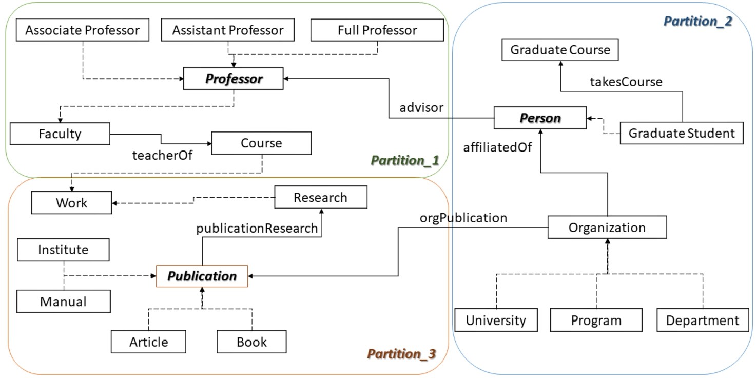
As a running example, Fig. 1 presents a fragment from the LUBM ontology and shows the three partitions that are formulated (
Fig. 1.
Dependence aware partitioning example for LUBM subset.
4.1.Importance measure for identifying centroids in the schema graph
Many measures have been produced for assessing the importance of the nodes in a knowledge graph and various notions of importance exist. When trying to group nodes from an RDF dataset, that are frequently queried together, according to our past exploration on centrality measures, the Betweenness Centrality (
In detail, the Betweenness Centrality of a schema node is equal to the number of the shortest paths from all schema nodes to all others that pass through that schema node. Formally:
Definition 4
Definition 4(Betweenness Centrality).
Let
Calculating the Betweenness for all nodes in a graph requires the computation of the shortest paths between all pairs of nodes. The complexity of the Brandes algorithm [6] for calculating it, is
As data distribution should also play a key role in estimating the importance of a schema node [31], we combine the value of
As such, the importance (
Definition 5
Definition 5(Importance Measure).
Let
REVFor calculating the number of instances of all schema nodes, we should visit all instances once, and as such the complexity of this part is
4.2.Assigning nodes to centroids using dependence
Having a way to assess the importance of the schema nodes using IM, we are next interested in identifying how to split data into partitions, i.e., to which partition the remaining schema nodes should be assigned. In order to define how dependent two schema nodes are, we introduce the Dependence measure.
Our first idea in this direction comes from the classical information theory, where infrequent words are more informative than frequent ones. The idea is also widely used in the field of instance matching [30]. The basic hypothesis here is that the greater the influence of a property on identifying a corresponding node, the fewer times the range of the property is repeated. According to this idea, we define Cardinality Closeness (
Definition 6
Definition 6(Cardinality Closeness of two adjacent schema nodes).
Let
The constant
Example 4.2.
Assume for example the schema nodes
Having defined the Cardinality Closeness of two adjacent schema nodes, we proceed further to identify the dependence. As such, we calculate the Dependence between two schema nodes, combining their Cardinality closeness, the IM of the schema nodes and the number of edges between them. Formally:
Definition 7
Definition 7(Dependence between two schema nodes).
Let
Intuitively, as we move away from a node, the dependence becomes smaller by calculating the differences of
Example 4.3.
Note also, that
5.DIAERESIS partitioning and query answering
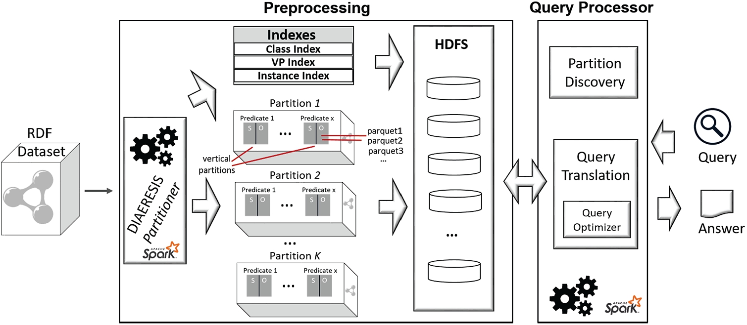
Figure 2 presents an overview of the DIAERESIS architecture, along with its internal components. Starting from the left side of the figure, the input RDF dataset is fed to the DIAERESIS Partitioner in order to partition it. For each one of the generated first-level partitions, vertical partitions are created and stored in the HDFS. Along with the partitions and vertical partitions, the necessary indexes are produced as well. Based on the available partitioning scheme, the DIAERESIS Query Processor receives and executes input SPARQL queries exploiting the available indexes. We have to note that although schema information is used to generate the first-level partitions, in the sequel the entire graph is stored in the system including both the instance and the schema graph. In the sequel, we will analyze in detail the building blocks of the system.
Fig. 2.
DIAERESIS overview.
5.1.The DIAERESIS partitioner
This component undertakes the task of partitioning the input RDF dataset, initially into first-level partitions, then into vertical partitions, and finally to construct the corresponding indexes to be used for query answering. Specifically, the Partitioner uses the Dependency Aware Partitioning (DAP) algorithm in order to construct the first-level partitions of data focusing on the structure of the RDF dataset and the dependence between the schema nodes. In the sequel, based on this first-level partitioning, instances are assigned to the various partitions, and the vertical partitions and the corresponding indexes are created.
5.1.1.Dependency aware partitioning algorithm
The Dependency Aware Partitioning (DAP) algorithm, given an RDF dataset V and a number of partitions k, splits the input dataset into k first-level partitions. The partitioning starts from the schema and then the instances follow. The algorithm splits the schema graph into sub-graphs, called first-level partitions, and then assigns the individuals in the partitions that they are instantiated under. Specifically, it uses the Importance Measure (IM) for identifying the partition’s centroids, and the Dependence for assigning nodes to the centroids where they belong. Depending on the characteristics of the individual dataset (e.g. it might be the case that most of the instances fall under just a few schema nodes), data might be accumulated into one partition, leading to data access overhead at query answering, as large fragments of data should be examined. DAP tries to achieve a balanced data distribution by reducing data access and maintaining a low replication factor.
Algorithm 1
DAP(V, k)
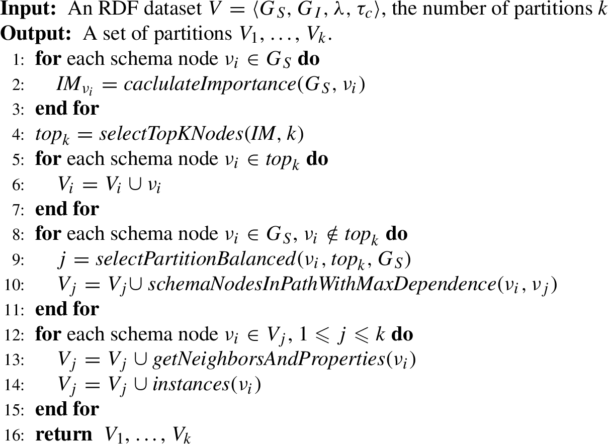
This is implemented in Algorithm 1, which starts by calculating the importance of all schema nodes (lines 1–3) based on the importance measure (IM) defined in Section 4.1, combining the betweenness centrality and the number of instances for the various schema nodes. Then, the k most important schema nodes are selected, to be used as centroids in the formulated partitions (line 4). The selected nodes are assigned to the corresponding partitions (lines 5–7). Next, the algorithm examines the remaining schema nodes in order to determine to which partition they should be placed based on their dependency on the partitions’ central nodes.
Initially, for each schema node, the dependence between the selected node and all centroids is calculated by the
However, we are not only interested in placing the selected schema node to the identified partition, but we also assign to that partition, all schema nodes contained in the path which connects the schema node with the selected centroid (line 10).
Then, we add the direct neighbors of all schema nodes in each partition along with the properties that connect them (line 13). Finally, instances are added to the schema nodes they are instantiated under (line 14). The algorithm terminates by returning the generated list of first-level partitions (line 16) containing the corresponding triples that their subject and object are located in the specific partitions.
Note that the aforementioned algorithm introduces replication (lines 12–15) that comes from the edges/properties that connect the nodes located in the different partitions. Specifically, besides allocating a schema node and the corresponding instances to a specific partition, it also includes its direct neighbors that might originally belong to a different partition. This step reduces access to different partitions for joins on the specific node.
Complexity. To identify the complexity of the algorithm, we should first identify the complexity of the various components involved. Assume
5.1.2.Vertical partitioning
Besides first-level partitioning, the DIAERESIS Partitioner also implements vertical sub-partitioning to further reduce the size of the data touched. Thus, it splits the triples of each partition produced by the DAP algorithm, into multiple vertical partitions, one per predicate, generating one file per predicate. Each vertical partition contains the subjects and the objects for a single predicate, enabling at query time a more fine-grained selection of data that are usually queried together. The vertical partitions are stored as parquet files in HDFS (see Fig. 2). A direct effect of this choice is that when looking for a specific predicate, we do not need to access the entire data of the first-level partition storing this predicate, but only the specific vertical partition with the related predicate. As we shall see in the sequel, this technique minimizes data access, leading to faster query execution times.
5.1.3.Number of first-level partitions
As already presented in Section 5.1.1, the DAP algorithm receives as an input the number of first-level partitions (k). This determines data placement and has a direct impact on the data access for query evaluation and the replication factor.
Based on the result data placement, as the number of partitions increases, the triples in the dataset might increase as well due to the replication of the triples that have domain/range in different partitions.
Theorem 1.
Let
Proof.
The theorem is immediately proved by construction (Lines 12–15 of the algorithm) as increasing the k will result in more schema nodes being split between the increased number of partitions, replicating all instances that span across the partitions. □
Interestingly, as the number of first-level partitions increases, the average number of data items located in each partition is reduced or at least stays the same since there are more partitions for data to be distributed in. Further, the data in the vertical sub-partitions decreases as well, i.e., even though the total number of triples might increase, on average, the individual subpartitions of
Theorem 2.
Let
Proof (sketch).
In order to prove this theorem, assume a partitioning for an RDF dataset
1. SC is placed in a partition where more schema nodes have one or more of the same predicates as SC. In this case, the number of triples of the vertical sub-partitions increases as more triples are added by the other schema nodes that have the same properties. However, although this happens locally, the schema node that is now in the same partition as SC is removed from the partition it was in the
2. SC is placed in a partition where fewer or the same schema nodes have one or more of the same predicates as SC. In this case, the number of triples of the vertical sub-partitions for SC is reduced or at least stays the same as in the
The aforementioned theorem has a direct impact on query evaluation as it actually tells us that if we increase k, the average data stored in the vertical sub-partitions, will be reduced or at least stay the same. This is verified also in the experimental evaluation (Section 6.2.3) showing the direct impact of k on both data replication and data access and as a result in query efficiency.
5.1.4.Indexing
Next, in order to speed up the query evaluation process, we generate appropriate indexes, so that the necessary sub-partitions are directly located during query execution. Specifically, as our partitioning approach is based on the schema of the dataset and data is partitioned based on the schema nodes, initially, we index for each schema node the first-level partitions (Class Index) it is primarily assigned to and also the vertical partitions (VP Index) it belongs. For each instance, we index also the schema nodes under which it is instantiated (Instance Index). The VP Index is used in case of a query with unbound predicates, in order to identify which vertical partitions should be loaded, avoiding searching all of them in a first-level partition.
The aforementioned indexes are loaded in the main memory of Spark as soon as the query processor is initialized. Specifically, the Instance Index, and the VP Index are stored in the HDFS as parquet files and loaded in the main memory. The Class Index is stored locally (txt file) since the size of the index/file is usually small and is also loaded in main memory at query processor initialization.
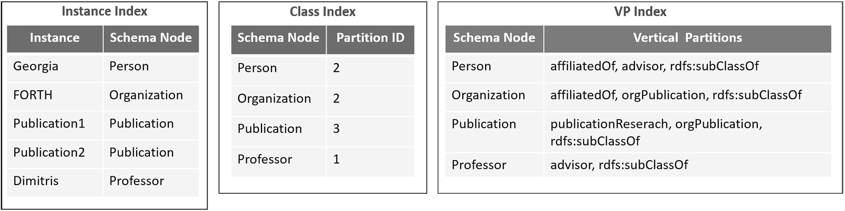
Example 5.1.
Fig. 3 presents example indexes for our running example. Assuming that we have five instances in our dataset, the Instance Index, shown in the figure (left), indexes for each instance the schema node to which it belongs. Further, the Class Index records for each schema node the first-level partitions it belongs, as besides the one that is primarily assigned, it might also be allocated to other partitions as well. Finally, the VP Index contains the vertical partitions that the schema nodes are stored into (for each first-level partition). For example, the schema node Organization (along with its instances) is located in Partition-2 and specifically its instances are located in the vertical partitions affiliatedOf, orgPublication and rdfs:subClassOf.
Fig. 3.
Instance, class and VP indexes for our running example.
5.2.Query processor
In this section, we focus on the query processor module, implemented on top of Spark. An input SPARQL query is parsed and then translated into an SQL query automatically. To achieve this, first, the Query Processor detects the first-level and vertical partitions that should be accessed for each triple pattern in the query, creating a Query Partitioning Information Structure. This procedure is called partition discovery. Then, this Query Partitioning Information Structure is used by the Query Translation procedure, to construct the final SQL query. Our approach translates the SPARQL query into SQL in order to benefit from the Spark SQL interface and its native optimizer which is enhanced to offer better results.
5.2.1.Partition discovery
Algorithm 2
PartitionDiscovery(query, classIndex, instanceIndex, VPIndex, stats)
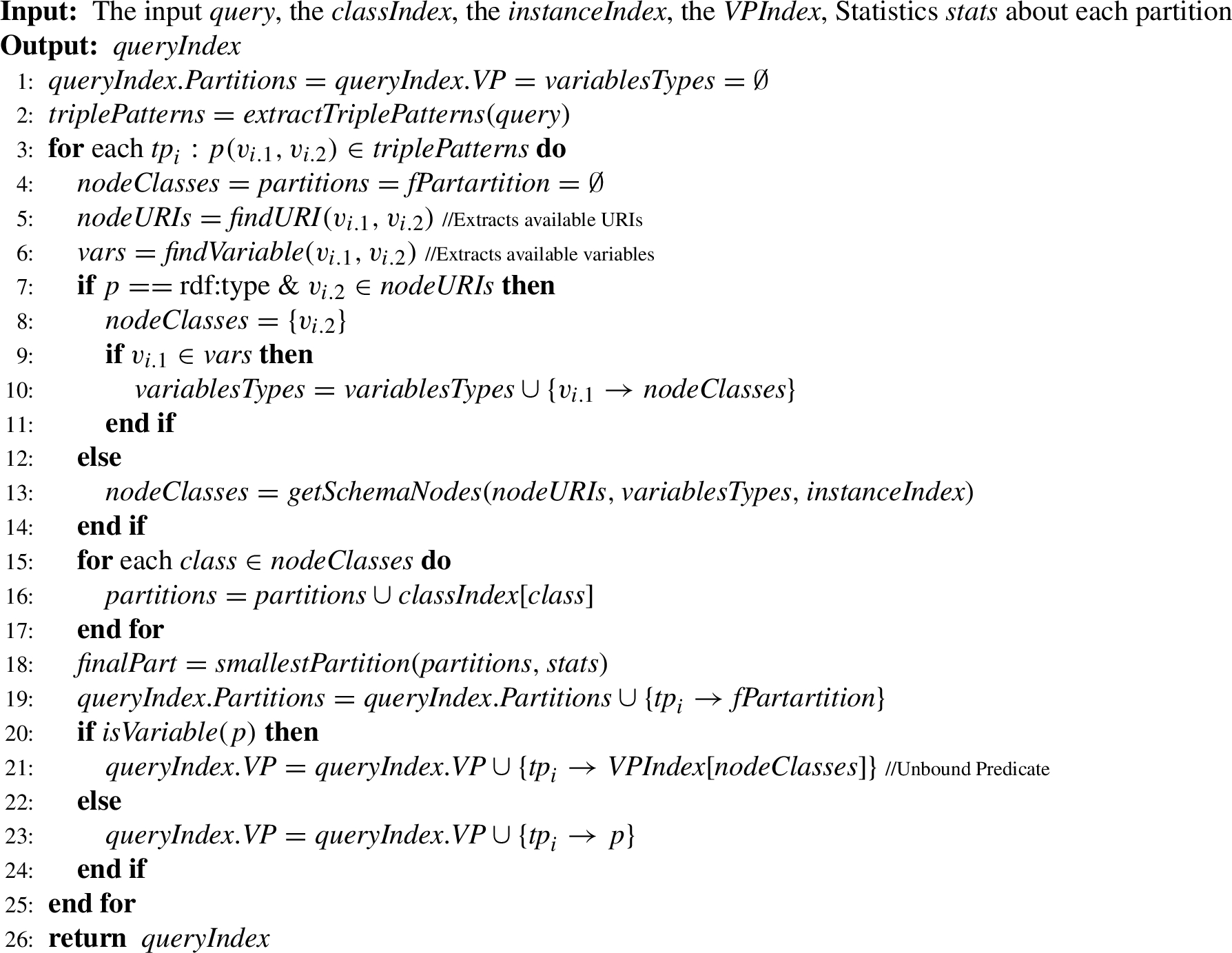
In the partition discovery module, we create automatically an index of the partitions that should be accessed for answering the input query, called Query Partitioning Information Structure. Specifically, we detect the fist-level partitions and the corresponding vertical partitions that include information to be used for processing each triple pattern of the query, exploiting the available indexes.
The corresponding algorithm, shown in Algorithm 2, takes as input a query, the indexes (presented in Section 5.1.4), and statistics on the size of the first-level partitions estimated during the partitioning procedure and returns an index of the partitions (first-level and vertical partitions) that should be used for each triple pattern.
The algorithm starts by initializing the variables
For each triple pattern the following variables are initialized (line 4):
While parsing each triple pattern, the node URIs (
A step further, the triple pattern is located in the vertical partition identified by the predicate of the triple pattern (lines 20–24). Specifically, in the case that the predicate of the triple pattern is a variable (we have an unbound predicate), the VP Index is used to obtain the set of vertical partitions based on the schema nodes (
Fig. 4.
Constructing query partitioning information structure.
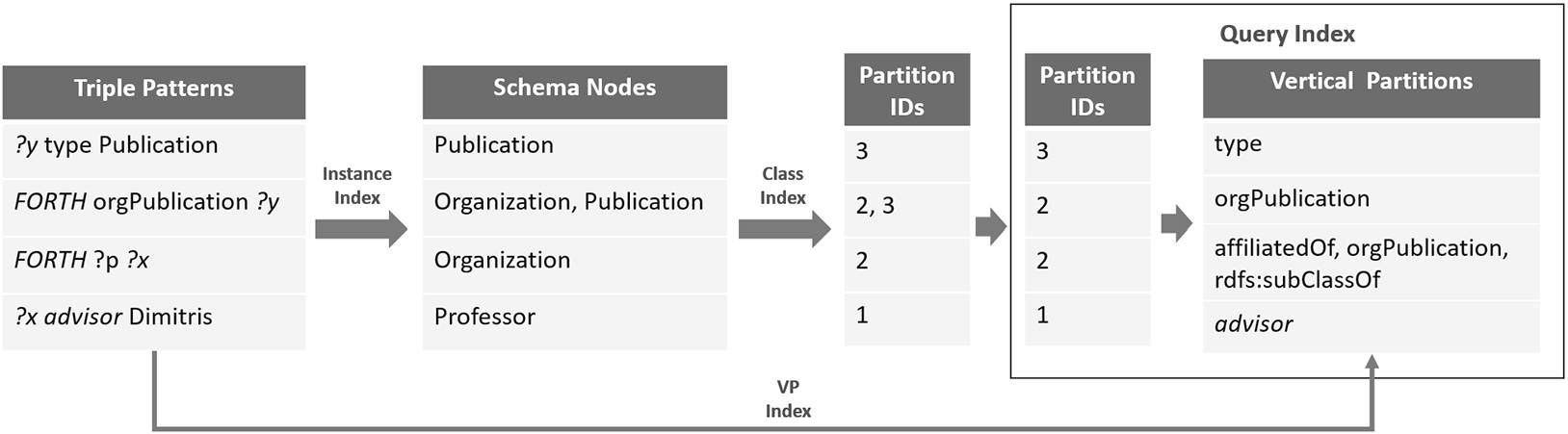
Example 5.2.
The creation of Query Partitioning Information Structure for a query is a three-step process depicted in Fig. 4. On the left side of the Figure, we can see the four triple patterns of the query. The first step is to map every triple pattern to its corresponding schema nodes. If a triple pattern contains an instance then the Instance Index is used to identify the corresponding schema nodes. Next by using the Class Index (Fig. 3), we find for each schema node the partitions where it is located in (Partitions IDs in Fig. 4). Finally we select the smallest partition in terms of size, for each schema node based on statistics collected for the various partitions. For example, for the second triple pattern (FORTH orgPublication ?y) we only keep the partition 2 since it is smaller than partition 3. For each one of the selected partitions, we finally identify the vertical partitions that should be accessed, based on the predicates of the corresponding triple patterns. In case of an unbound predicate, such as in the third triple pattern of the query (FORTH ?p ?x) in Fig. 4, the VP Index is used to identify the vertical partitions in which this triple pattern could be located based on its first-level partition (Partition ID:2). The result Query Partitioning Information Structure for our running example is depicted on the right of Fig. 4.
5.2.2.Query translation & optimization
In order to produce the final SQL query, each triple pattern is translated into one SQL sub-query. Each one of those sub-queries specifically involves a vertical sub-partitioning table based on the predicate name – the table name in the “FROM” clause of the SQL query. For locating this table the Query Partitioning Information Structure is used. Afterward, all sub-queries are joined using their common variables.
Finally, in order to optimize query execution we disabled default query optimization by Spark as in many cases the returned query plans were not efficient and we implemented our own optimizer. Our optimizer exploits statistics recorded during the partitioning phase, to push joins on the smallest tables – in terms of rows – to be executed first, further boosting the performance of our engine. The query translation and optimization procedures are automatic procedures performed at query execution.
Fig. 5.
Query translation.
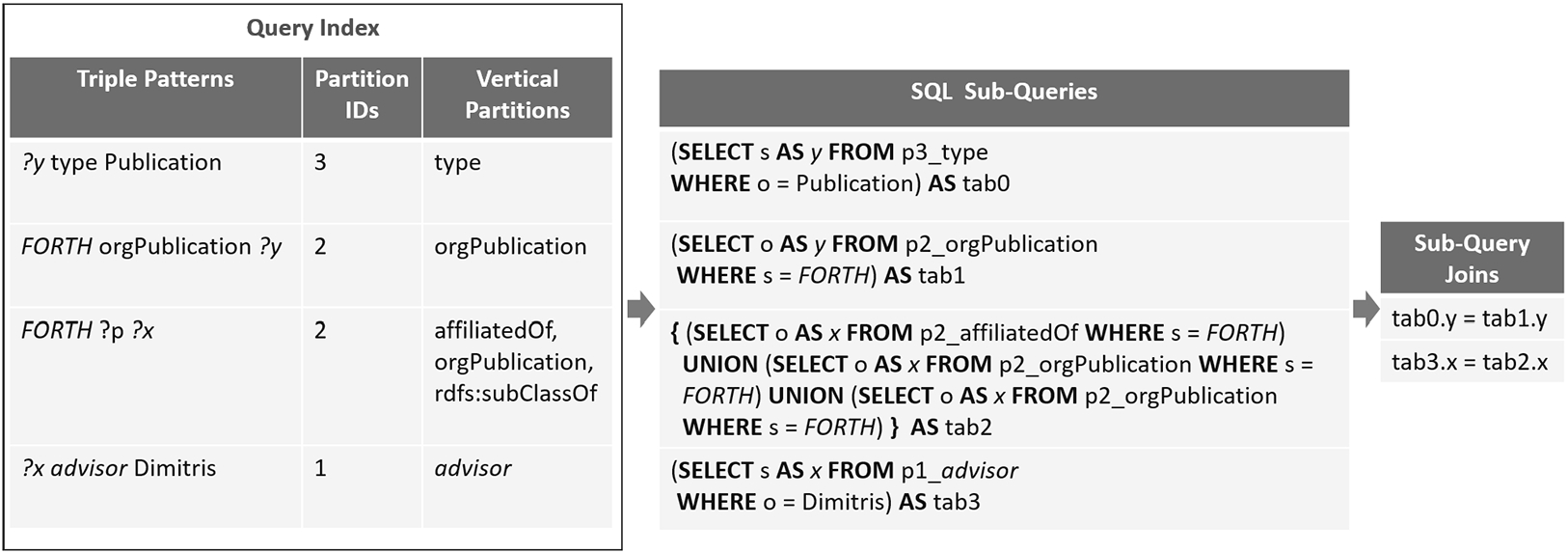
Example 5.3.
In Fig. 5, an example is shown of the query processor module in action. The input of the translation procedure is the Query Partitioning Information Structure of Fig. 4. Each triple pattern is translated into an SQL query, based on the corresponding information for the first-level and vertical partitions (SQL Sub-Queries in Fig. 5) that should be accessed. The name of the table of each SQL query is the concatenation of the first-level and the vertical partitions. In case of an unbound predicate, such as the third triple pattern, the sub-query asks for more than one table based on the vertical partitions that exist in the Query Partitioning Information Structure for the specific triple pattern. Finally, sub-queries are reordered by the DIAERESIS optimizer that pushes joins on the smallest tables to be executed first – in our example the p3_type is first joined with p2_orgPublication.
6.Evaluation
In this section, we present the evaluation of our system. We evaluate our approach in comparison to three query processing systems based on Spark, i.e., SPARQLGX [12], S2RDF [29], and WORQ [23], using two real-world RDF datasets and four versions of a synthetic dataset, scaling up to 1 billion triples.
6.1.System setup
LUBM. The Lehigh University Benchmark (LUBM) [13] is a widely used synthetic benchmark for evaluating semantic web repositories. For our tests, we utilized the LUBM synthetic data generator to create four datasets of 100, 1300, 2300, and 10240 universities (LUBM100, LUBM1300, LUBM2300, LUBM10240) occupying 2.28 GB, 30.1 GB, 46.4 GB, 223.2 GB, and consisting of 13.4M triples, 173.5M triples, 266.8M triples, and 1.35B triples respectively. LUBM includes 14 classes and 18 predicates. We used the 14 queries provided by the benchmark for our evaluation, each one ranging between one to six triple patterns. We classify them into three categories, namely, star, chain, snowflake, and complex queries.
SWDF. The Semantic Web Dog Food (SWDF) [24] is a real-world dataset containing Semantic Web conference metadata about people, papers, and talks. It contains 126 classes, 185 predicates, and 304,583 triples. The dataset occupies 50 MB of storage. To evaluate our approach, we use a set of 278 BGP queries generated by the FEASIBLE benchmark generator [27] based on real query logs. In the benchmark workload, all queries include unbound predicates. Although our system is able to process them, no other system was able to execute them. As such, besides the workload with the unbound predicates (noted as SWDB(u)), we also replaced the unbound predicates with predicates from the dataset (noted as SWDF(b)) to be able to compare our system with the other systems, using the aforementioned workload.
DBpedia. Version 3.8 of DBpedia, contains 361 classes, 42,403 predicates, and 182,781,038 triples. The dataset occupies 29.1 GB of storage. To identify the quality of our approach, we use a set of 112 BGP queries generated again by the FEASIBLE benchmark generator based on real query logs. As it is based on real query logs the query workload here is closer to the queries of real users instead of focusing on the system’s choke points – usually the focus of the synthetic benchmarks. As such they contain a smaller number of triple patterns as reported also by relevant papers in the domain [5].
All information about the datasets is summarized in Table 2. Further, all workloads along with the code of the system are available in our GitHub repository.11
Table 2
Dataset statistics
| Dataset | #Triples | Size (.nt) | #Classes | #Predicates |
| LUBM 100 | 13,405,381 | 2.28 GB | 14 | 18 |
| LUBM 1300 | 173,546,369 | 30.1 GB | 14 | 18 |
| LUBM 2300 | 266,814,882 | 46.4 GB | 14 | 18 |
| LUBM 10240 | 1,340,300,979 | 223.2 GB | 14 | 18 |
| SWDF | 304,583 | 49.2 MB | 126 | 185 |
| DBpedia | 182,781,038 | 29.1 GB | 361 | 42,403 |
6.1.1.Setup
Our experiments were conducted using a cluster of 4 physical machines that were running Apache Spark (3.0.0) using Spark Standalone mode. Each machine has 400 GB of SSD storage, and 38 cores, running Ubuntu 20.04.2 LTS, connected via Gigabit Ethernet. In each machine, 10 GB of memory was assigned to the memory driver, and 15 GB was assigned to the Spark worker for querying. For DIAERESIS, we configured Spark with 12 cores per worker (to achieve a total of 48 cores), whereas we left the default configuration for other systems.
6.1.2.Competitors
Next, we compare our approach with three state-of-the-art query processing systems based on Spark, i.e., the SPARQLGX [12], S2RDF [29], and WORQ [23]. In their respective papers, these systems have been shown to greatly outperform SHARD, PigSPARQL, Sempala and Virtuoso Open Source Edition v7 [29]. We also made a consistent effort to get S3QLRDF [15,16] in order to include it in our experiments, however access to the system was not provided.
SPARQLGX implements a vertical partitioning scheme, creating a partition in HDFS for every predicate in the dataset. In the experiments we use the latest version of SPARQLGX 1.1 that relies on a translation of SPARQL queries into executable Spark code that adopts evaluation strategies to the storage method used and statistics on data. S2RDF, on the other hand, uses Extended Vertical Partitioning (ExtVP), which aims at table size reduction,when joining triple patterns as semijoins are already precomputed. In order to manage the additional storage overhead of ExtVP, there is a selectivity factor (SF) of a table in ExtVP, i.e. its relative size compared to the corresponding VP table. In our experiments, the selectivity factor (SF) for ExtVP tables is 0.25 which the authors propose as an optimal threshold to achieve the best performance benefit while causing only a little overhead. Moroever, the latest version of S2RDF 1.1 is used that supports the use of statistics about the tables (VP and ExtVP)) for the query generation/evaluation. Finally, WORQ [23](version 0.1.0) reduces sets of intermediate results that are common for certain join patterns, in an online fashion, using Bloom filters, to boost query performance.
Regarding compression, all systems use parquet files to store VP (ExtVP) tables that enable better compression, and also WORQ uses dictionary compression.
DIAERESIS, S2RDF, and WORQ exploit the caching functionality of Spark SQL. As such, we do not include caching times in our reported query runtimes as it is a one-time operation not required for subsequent queries accessing the same table. SPARQLGX, on the other hand, loads the necessary data for each query from scratch so the reported times include both load time and query execution times. Further, we experimentally determined the number of partitions k that achieves an optimal trade-off between storage replication and query answering time. More details about the number of first-level partitions and how it affects the efficiency of query answering and the storage overhead can be found in Section 6.2.3. As such LUBM 100, LUBM 1300, LUBM 2300, and SWDF were split into 4 first-level partitions, LUBM 10240 into 10 partitions, and DBpedia into 8 partitions. Finally, note that a time-out of one week was selected for all the experiments, meaning that after one week without finishing the execution, each individual experiment was stopped.
Table 3
Preprocessing dimensions
| System | Preprocessing time | Output storage | Replication factor |
| LUBM 100 (13.4M triples) | |||
| SPARQLGX | 0.73 min | 101.52 MB | 0.33 |
| S2RDF | 8.21 min | 332.3 MB | 1.10 |
| WORQ | 2.16 min | 73.19 MB | 0.24 |
| DIAERESIS | 8.12 min | 336.07 MB | 1.12 |
| LUBM 1300 (173.5M triples) | |||
| SPARQLGX | 4.91 min | 1.48 GB | 0.35 |
| S2RDF | 25.76 min | 4.39 GB | 1.05 |
| WORQ | 21.71 min | 0.86 GB | 0.21 |
| DIAERESIS | 124.31 min | 4.74 GB | 1.14 |
| LUBM 2300 (266.8M triples) | |||
| SPARQLGX | 7.55 min | 2.30 GB | 0.35 |
| S2RDF | 36.63 min | 6.84 GB | 1.06 |
| WORQ | 33.96 min | 1.32 GB | 0.21 |
| DIAERESIS | 130.07 min | 6.89 GB | 1.06 |
| LUBM 10240 (1.35 billion triples) | |||
| SPARQLGX | 64.6 min | 12.42 GB | 0.38 |
| S2RDF | 175.61 min | 33.99 GB | 1.04 |
| WORQ | 275.49 min | 9.54 GB | 0.29 |
| DIAERESIS | 187.44 min | 44.32 GB | 1.36 |
| SWDF (304K triples) | |||
| SPARQLGX | 0.45 min | 5.38 MB | 0.40 |
| S2RDF | 15 min | 44.58 MB | 3.31 |
| WORQ | 2.3 min | 6.05 MB | 0.45 |
| DIAERESIS | 2.5 min | 11.59 MB | 0.86 |
| DBpedia (182M triples) | |||
| SPARQLGX | 3.7 min | 3.7 GB | 0.41 |
| S2RDF | Timeout | - | - |
| WORQ | Timeout | - | - |
| DIAERESIS | 273.56 min | 16.7 GB | 2.41 |
6.1.3.Preprocessing
In the preprocessing phase, the main dimensions for evaluation are the time needed to partition the given dataset and the storage overhead that every system introduces in terms of the Replication Factor (RF). Specifically, RF is the number of copies of the input dataset each system outputs in terms of raw compressed parquet file sizes. Table 3 presents the results for the various datasets and systems.
Preprocessing time. Focusing, initially, on the time needed for each system to partition the dataset, we can observe that SPARQLGX has almost in all cases the fastest preprocessing time. This is due to the fact that it implements the most naive preprocessing procedure, as it aggregates data by predicates and then creates a compressed folder for every one of these predicates. However, exactly due to this simplistic policy, large fragments of data are required for query-answering as we will show in Section 6.2.1. S2RDF partitions 13.4M triples (LUMB 100) faster than 304K (SWDF) ones. This happens as LUBM, being a synthetic dataset, has only 18 predicates, compared to SWDF which has 185. Regarding preprocessing time for the other LUBM datasets, S2RDF shows an almost linear increase. In the case of DBpedia, which has 42,403 predicates and is relatively big, both S2RDF and WORQ fail to preprocess it. More precisely, S2RDF was returning an error failing to process the complex structure of DBpedia, whereas the WORQ preprocessing stage was running for more than a week without returning results. Besides DBpedia, WORQ has relatively good preprocessing time for the remaining datasets showing also an almost linear increase in preprocessing time as the data grow. DIAERESIS requires more preprocessing time to finish, since it employs a more sophisticated algorithm. However, it is not stalled by complex datasets, such as WORQ and S2RDF. Nevertheless preprocessing is a task that is only executed once and offline for all systems before starting to answer queries.
Replication. By further examining the results shown in Table 3, SPARQLGX has no replication overhead since, as already explained, it is implementing a naive vertical partitioning schema. In fact, as information is omitted from the generated vertical partitions (i.e. the predicates), the result dataset is even smaller than the input. S2RDF, on the other hand, precomputes both the VP tables and every other possible semi-join combination of the dataset (up to a limit). This results in storage overhead. Regarding WORQ, again the result of preprocessed data is smaller than the initial dataset since it uses dictionary compression.
Looking at Table 3, for the LUBM datasets, the replication factor of SPARQLGX is around 0.35, for WORQ ranges between 0.21 and 0.29, for S2RDF is around 1.05, whereas for our approach it ranges between 1.05 and 1.36.
For the SWDF dataset, we see that SPARQLGX and WORQ have a replication factor of around 0.4, S2RDF has a replication factor of 3.31 due to the big amount of predicates contained in the dataset, whereas our approach has 0.86, achieving a better replication factor than S2RDF in this dataset, however falling behind the simplistic partitioning methods of SPARQLGX. That is, placing dependent nodes together, sacrifices storage overhead, for drastically improving query performance.
Overall, SPARQLGX wins in terms of preprocessing time in most of the cases due to its simplistic partitioning policy, however with a drastic overhead in query execution as we shall see in Section 6.2.1. On the other hand, S2RDF and WORQ fail to finish partitioning on a complex real dataset.
Nevertheless, we argue that preprocessing is something that can be implemented offline without affecting overall system performance and that a small space overhead is acceptable for improving query performance.
6.2.Query execution
Next, we evaluate the query execution performance for the various systems. The times reported are the average of 10 executions of each set of queries. Note that the times presented concern only the execution times for DIAERESIS, S2RDF, and WORQ (as they use the cache to pre-load data), whereas for SPARQLGX include both loading and execution times as these steps cannot be separated in query answering.
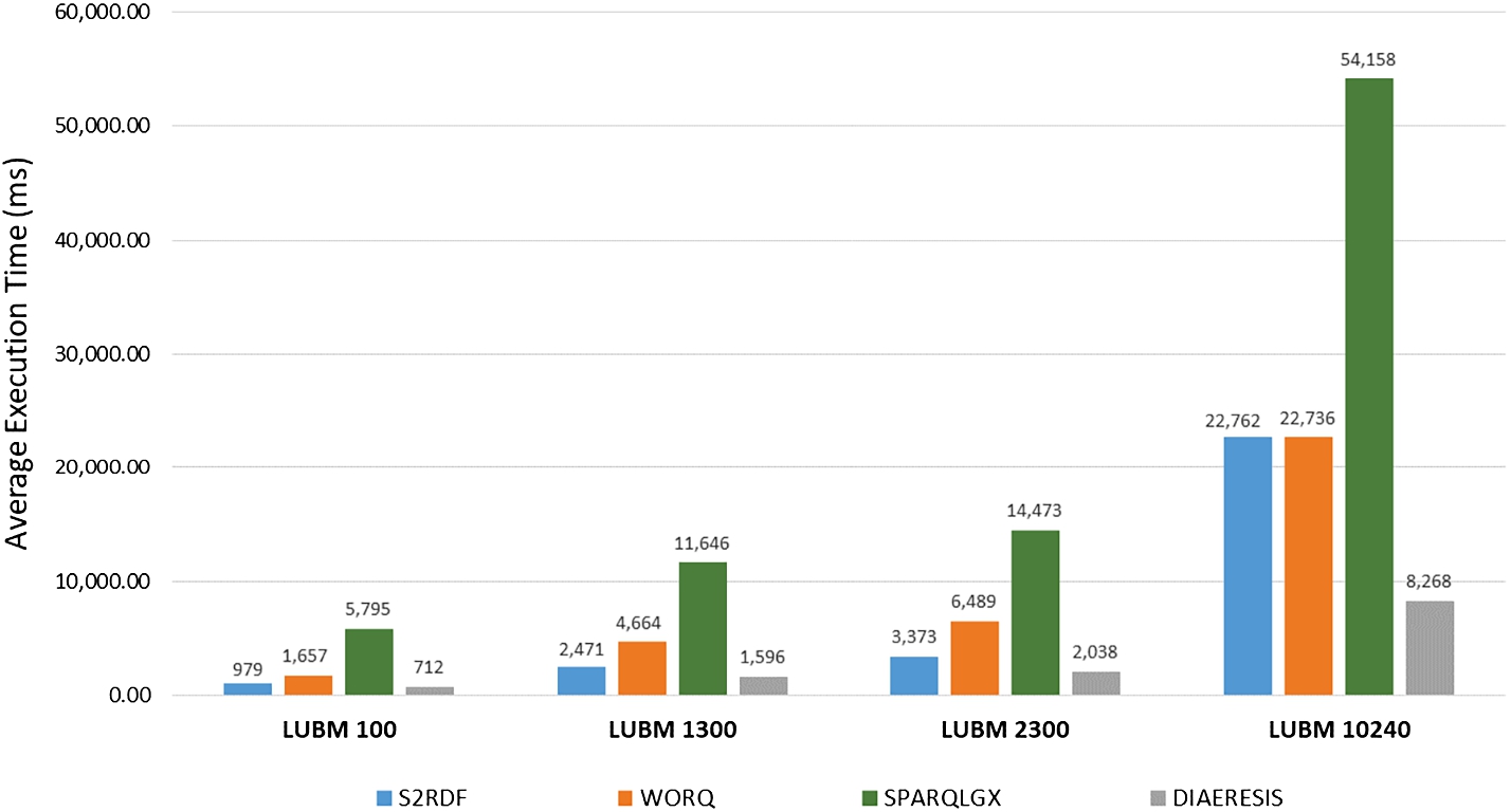
Fig. 6.
Query execution for LUBM datasets and systems.
6.2.1.LUBM
In this experiment, we show how the performance of the systems changes as we increase the dataset size using the four LUBM datasets – ranging from 13 million to 1.35 billion triples.
Figure 6 compares the average query execution time of different systems for the LUBM datasets. We can observe that in all cases, our system strictly dominates the other systems. More importantly, as the size of the dataset increases, the difference in the performance between DIAERESIS and the other systems increases as well. Specifically, our system is one order of magnitude faster than all competitors for LUBM100 and LUBM10240. For LUBM1300, DIAERESIS is two times faster than the most efficient competitor, whereas for LUBM2300, DIAERESIS is 40% faster than the most efficient competitor.
DIAERESIS continues to perform better than the other systems in terms of average query execution time across all versions, enjoying the smallest increase in execution times, compared to the other systems, as the dataset grows. For the largest dataset, i.e., LUBM10240, our system outperforms the other systems, being almost three times faster than the most efficient competitor. This demonstrates the superiority of DIAERESIS in big datasets. We conclude that as expected, the size of the dataset affects the query execution performance. Generally, SPARQLGX has the worst performance since it employs a really naive partitioning scheme, followed by S2RDF and WORQ – only in LUBM1024, WORQ is better than S2RDF. In contrast, the increase in the dataset size has the smallest impact for DIAERESIS, which dominates competitors.
Fig. 7.
Query execution for (a) LUBM 100, (b) LUBM 1300, (c) LUBM 2300, (d) LUBM 10240.
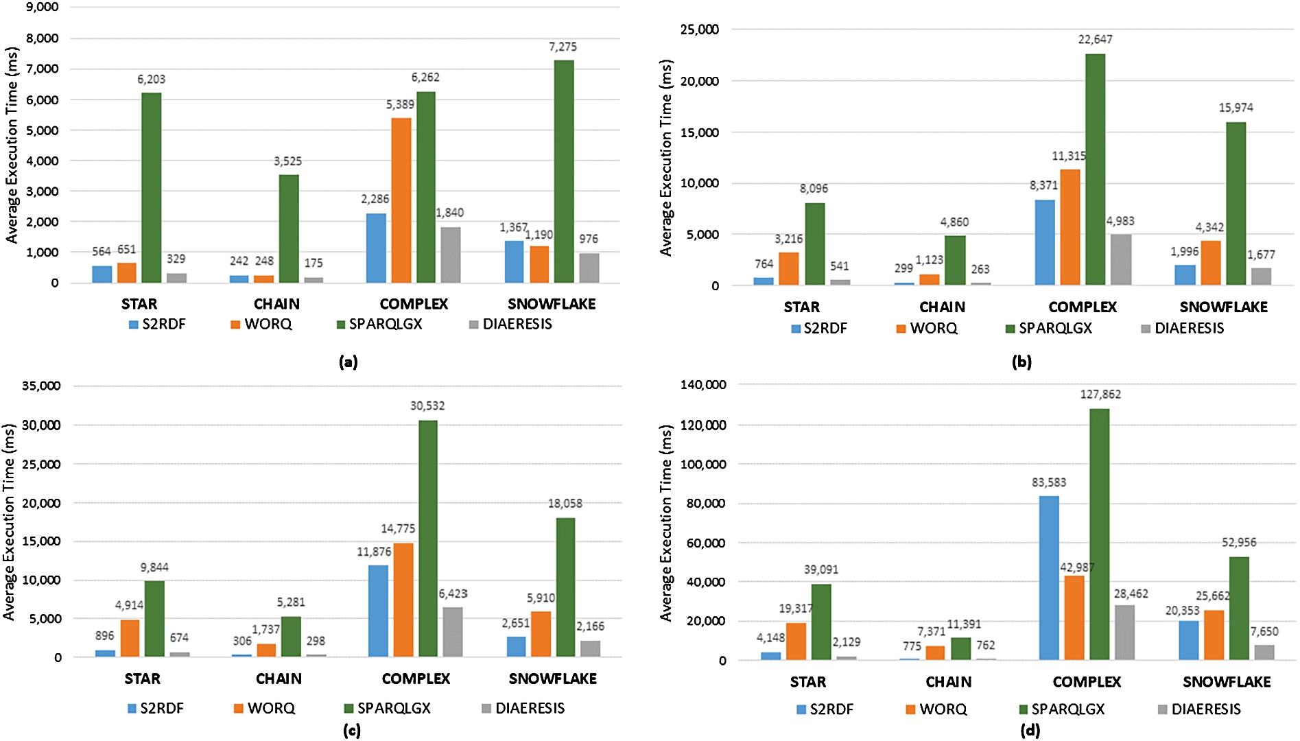
Query Categories. Next, we study separately the four types of queries available, i.e., star, chain, snowflake, and complex queries. Their execution times are presented in Fig. 7. Regarding star queries, we notice that for all LUBM datasets, DIAERESIS has the best performance followed by S2RDF, WORQ, and in the end SPARQLGX with a major difference. S2RDF performs better than WORQ due to the materialized join reduction tables since it uses fewer data to answer most of the queries than WORQ, as we will see in the sequel. Since our system places together dependent fragments of data that are usually queried together, it is able to reduce data access for query answering, performing significantly better than competitors.
For chain queries (Fig. 7), the competitors perform quite well except for SPARQLGX which performs remarkably worse. More precisely, S2RDF performs slightly better than WORQ except for the LUBM100, the smallest LUBM dataset, where the difference is negligible. Still, DIAERESIS delivers a better performance than the other systems in this category for all LUBM datasets.
The biggest difference between DIAERESIS and the competitors is observed in complex queries for all LUBM datasets (Fig. 7). Our system is able to lead to significantly better performance, despite the fact that this category contains the most time-demanding queries, with the bigger number of query triple patterns, and so joins. The difference in the execution times between our system and the rest becomes larger as the size of the dataset increases. S2RDF has the second better performance followed by WORQ and SPARQLGX in LUBM100, LUBM1300 and LUBM2300. However in LUBM10240 S2RDF comes third since WORQ is quite faster and SPAQGLGX is the last one. S2RDF performs better than WORQ due to the materialized join reduction tables since S2RDF uses fewer data to answer the queries than WORQ in all cases However, as the data grow, i.e., in LUBM10240, the complex queries with many joins, perform better in WORQ than S2RDF due to the increased benefit of the bloom filters.
Finally, in snowflake queries, again we dominate all competitors, whereas S2RDF in most cases comes second, followed by WORQ and SPAQLGX. Only in the smallest dataset, i.e. LUBM100, WORQ has a better performance. Again SPARQLGX has the worst performance in all cases.
The value of our system is that it reduces substantially the accessed data in most of the cases as it is able to retain the same partition dependent schema nodes that are queried together along with their corresponding instances. This will be subsequently presented in the section related to the data access reduction.
Fig. 8.
Query execution for (a) LUBM 100, (b) LUBM 1300, (c) LUBM 2300, (d) LUBM 10240.
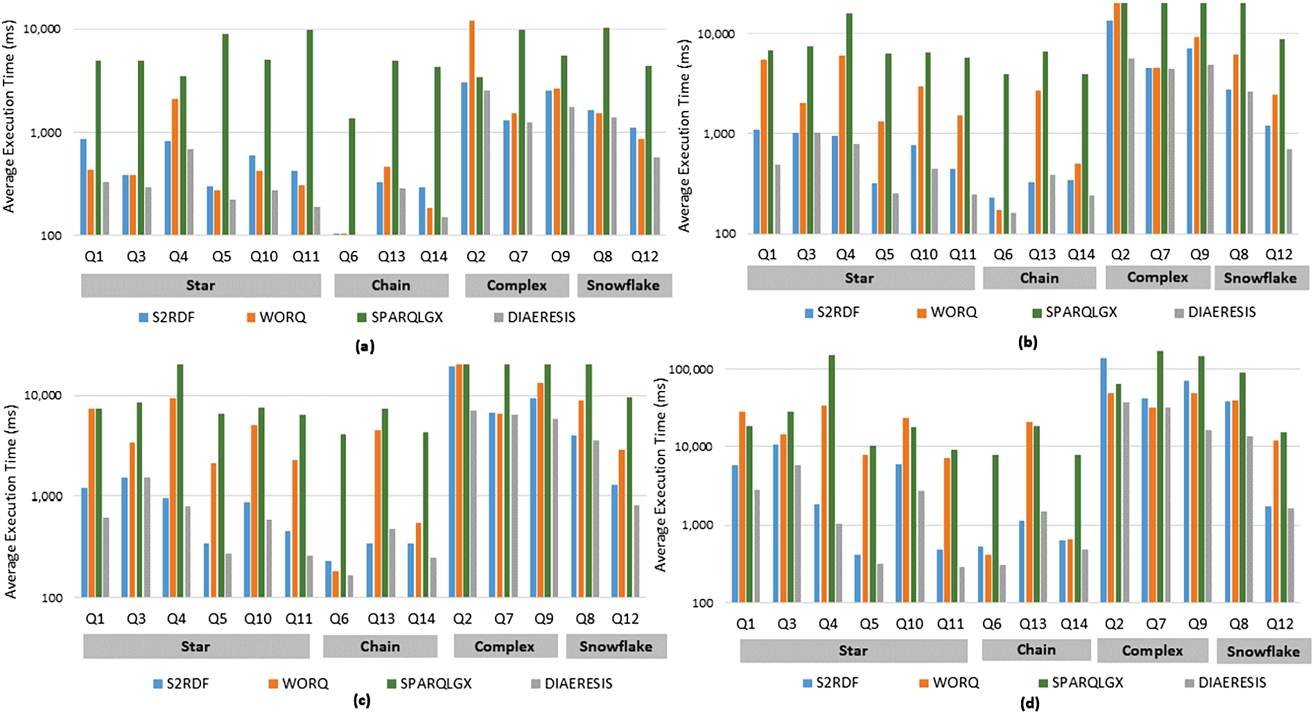
Individual Queries. Examining closely the individual queries and their execution times (Fig. 8), for the star queries, DIAERESIS dominates other systems in all star queries for all LUBM datases. On the other hand, S2RDF wins WORQ in all LUBM datesets, except LUBM100 that it performs worse in five queries out of the total six star queries – except Q4 which is the only one in this category that has three joins while the others have one join.
Regarding chain queries, DIAERESIS outperforms the competitors on all individual chain queries, except Q13 in LUBM1300, LUBM2300 and LUBM 10240 where S2RDF is slightly better. This happens as S2RDF has already precomputed the two joins required for query answering and as such despite the fact that DIAERESIS loads fewer data (according to Fig. 9) the time spent in joining those data is higher than just accessing a bigger number of data. For Q6, WORQ performs better than S2RDF in all LUBM datasets. However, for Q14, S2RDF wins WORQ in LUBM1300, LUBM230, and slightly in LUBM10240, while WORQ is significantly faster than S2RDF in LUBM100.
Complex and snowflake queries put a heavy load on all systems since they consist of many joins (3–5 joins). DIAERESIS continues to demonstrate its superior performance and scalability since it is faster than competitors to all individual queries for all LUBM datasets. Competitors on the other hand do not show stability in their results. S2RDF comes second followed by WORQ and then SPARQLGX, in terms of execution time for most of the queries of the complex category, except LUBM10240. Specifically, for the biggest LUBM dataset, WORQ wins S2RDF in all complex queries apart from one. In the snowflake category, WORQ is better in LUBM100 and in LUBM10340 but not in the rest.
Fig. 9.
Reduction of data access for LUBM10240.
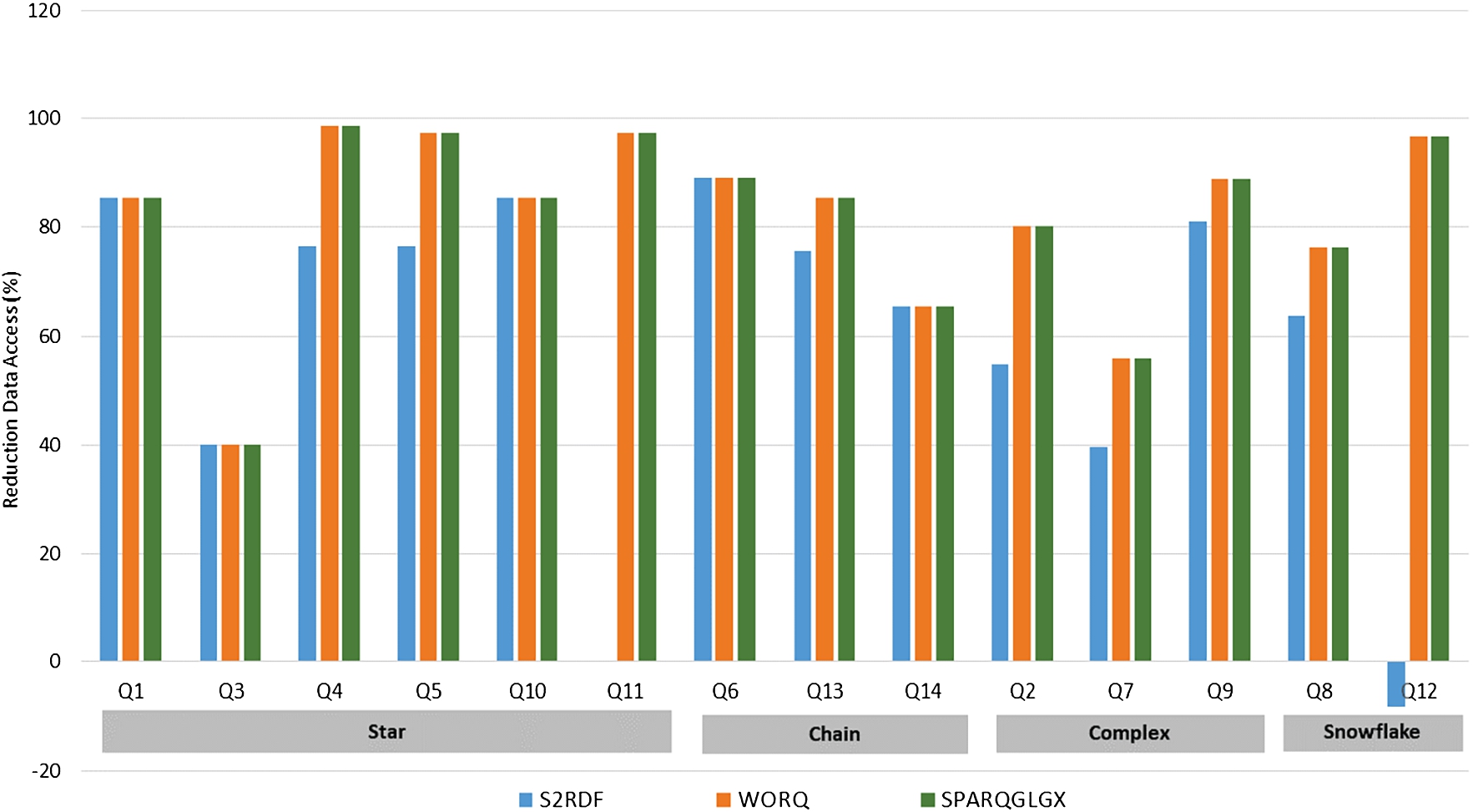
Data Access Reduction. Moving to explain the large performance improvement of our system, we present next the percentage of the reduction in the size of the data accessed for query answering for all systems when compared to DIAERESIS for each individual query for LUBM10240 (refer to Fig. 9).
To evaluate data access reduction we use the following formula:
The formula calculates the percentage of the difference between the total rows accessed by the competitors and the total rows accessed by DIAERESIS for each query. The rows can be easily measured by summing the number of rows of all the vertical partition tables loaded/used for answering a query.
We only present LUBM10240 as the graphs for the other versions are similar. As shown, our system consistently outperforms all competitors, and in many cases to a great extent. DIAERESIS accesses 99% less data than WORQ for answering Q4, whereas for many queries the reduction is over 90%. For S2RDF on the other hand, the reduction in most of the cases is more than 60%. In only one case (Q12), our system loads 8.12% more data than S2RF, as the reduction tables used by S2RDF are smaller than the subpartitions loaded by DIAERESIS. However, even at that case, DIAERESIS performs better in terms of query execution time due to the most effective query optimization procedures we adopt, as shown already in Fig. 8. Note that although in five cases the data access reduction of S2RDF, WORQ, and SPARQLGX when compared to DIAERESIS seems to be the same (Q1, Q3, Q10, Q6, Q14) as shown in Fig. 9, S2RDF performs better that WORQ and SPARQLGX due to the query optimization it performs. Regrading SPARQLGX, in the most of the cases, the percentage of the reduction is over 80%, and in many cases over 90%.
Overall we can conclude that DIAERESIS boosts query performance, while effectively reducing the data accessed for query answering.
6.2.2.Real-world datasets
Fig. 10.
Query execution for real-world datasets and systems.
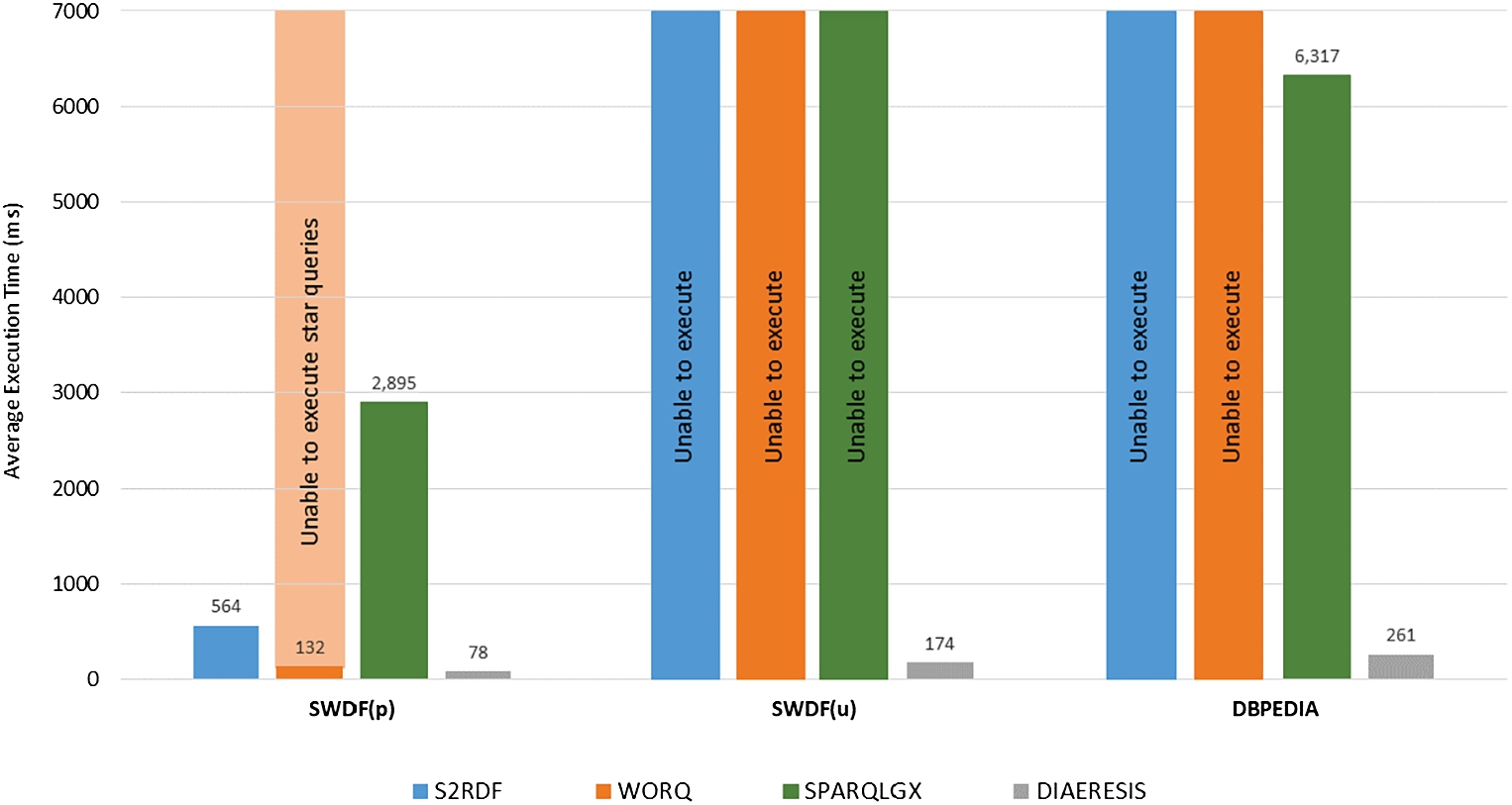
Apart from the synthetic LUBM benchmark datasets, we evaluate our system against the competitors over two real-world datasets, i.e., SWDF (unbound and bound) and DBpedia (Fig. 10).
As already mentioned, no other system is able to execute queries with unbound predicates (i.e., SWDF(u)) in Fig. 10), whereas for the SWDF workload with bound predicates (277 queries) (i.e., SWDF(b) in Fig. 10) our system is one order of magnitude faster than competitors. WORQ was not able to execute star queries (147 queries) in this dataset, since the triples of star queries for this specific dataset should be joined through constants instead of variables as usual. Regarding DBpedia (Fig. 10), both S2RDF and WORQ failed to finish the partitioning procedure due to the large number of predicates contained in the dataset and the way that the algorithms of the systems use this part.
Fig. 11.
Query execution for (a) SWDF(p), (b) DBpedia.
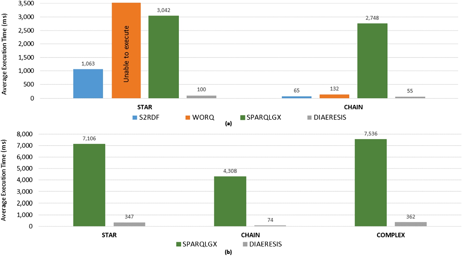
Query Categories. Examining each query category in Fig. 11, we can verify again that DIAERESIS strictly dominates other systems in all query categories as well. More specifically, DIAERESIS is one order of magnitude faster in star and complex queries than the fastest competitor able to process these datasets. The SWDF workload did not contain complex queries, whereas for the DBpedia dataset for complex queries, DIAERESIS is again one order of magnitude faster than SPARQLGX.
Overall, the evaluation clearly demonstrates the superior performance of DIAERESIS in real datasets as well, when compared to the other state-of-the-art partitioning systems, for all query types. DIAERESIS does not favour any specific query type, achieves consistent performance, dominating all competitors in all datasets.
6.2.3.Impact of the number of the first-level partitions
Table 4
Comparing DIAERESIS and competitors for different number of first-level partitions (k)
| System | Partitions | Replication factor | Data access (M rows) | Execution time |
| LUBM 10240 | ||||
| DIAERESIS | 4 | 1.32 | 2, 531 | 179,357 ms |
| DIAERESIS | 6 | 1.35 | 2, 509 | 160,189 ms |
| DIAERESIS | 8 | 1.35 | 1, 460 | 147,203 ms |
| DIAERESIS | 10 | 1.36 | 1, 406 | 116,908 ms |
| SPARQLGX | 0.38 | 7, 510 | 758,218 ms | |
| S2RDF | 1.04 | 4, 348 | 318,668 ms | |
| WORQ | 0.29 | 7, 510 | 318,299 ms | |
| DBpedia | ||||
| DIAERESIS | 4 | 1.83 | 353 | 37,731 ms |
| DIAERESIS | 6 | 2.20 | 242 | 32,635 ms |
| DIAERESIS | 8 | 2.41 | 184 | 20,777 ms |
| DIAERESIS | 10 | 2.50 | 145 | 18,650 ms |
| SPARQLGX | 0.41 | 925 | 599,134 ms | |
In this subsection, we experimentally investigate the influence of the number of first-level partitions on storage overhead, data access for query evaluation, and query efficiency verifying the theoretical results presented in Section 5.1.3.
For this experiment, we focus on the largest synthetic and real-world datasets, i.e. LUBM10240 and DBpedia, since their large size enables us to better understand the impact of the number of first-level partitions on the data layout and the query evaluation. We compare the replication factor, the total amount of data accessed for answering all queries in the workload in terms of number of rows, and the total query execution time varying the number of first-level partitions between four and ten for the two datasets.
The results are presented in Table 4 for the various DIAERESIS configurations and we also include the competitors able to run in these datasets.
For both datasets, we notice that as the number of first-level partitions increases, the replication factor increases as well. This confirms empirically Theorem 1 (Section 4), which tells us that as the number of partitions increases, the total storage required might increase as well.
The rate of the increase in terms of storage is larger in DBpedia than in LUBM10240 since the number of properties in DBpedia is quite larger compared to LUBM10240 (42.403 vs 18). The larger number of properties in DBpedia results in more properties spanning between the various partitions and, as such, increases the replication factor.
Further, looking at the total data access for query answering, we observe as well that the larger the number of partitions the smaller the data required to be accessed for answering all queries. This empirically confirms also Theorem 2 (Section 4) which tells us that the more the partitions the smaller the data required for query answering in terms of total data accessed. The reduced data access has also a direct effect on query execution which is reduced as K increases.
Compering DIAERESIS performance with the other competitors, we can also observe that they access a larger fragment of data for answering queries in all cases, which is translated into a significantly larger execution time.
6.2.4.Example query
In order to illustrate the impact of the number of the first-level partitions we present in detail a query from the LUBM benchmark (Q3) on the LUBM10240 dataset. This query belongs in the star queries category and returns six results as an answer. The query is shown in the sequel and retrieves the publications of
PREFIX swat: <http://swat.cse.lehigh.edu/onto/univ-bench.owl/>
PREFIX dep: <http://www.Department0.University0.edu/>

Q3: SELECT ?X  WHERE{
    ?X rdfs:type swat:Publication.
    ?X swat:publicationAuthor dep:AssistantProfessor0 .
}
In DIAERESIS, the query is translated in the following query for a
X SELECT tab1.X AS X FROM
    (SELECT s AS X FROM part7_type
        WHERE o == ’swat:Publication’) AS tab0,
    (SELECT s AS X FROM part7_publicationauthor
        WHERE o == ’dep:AssistantProfessor0’) AS tab1
WHERE tab0.X=tab1.X
Table 5
Data access and execution time for various k for the Q3 query of the LUBM benchmark
| Partitions | Data access (rows) | Execution time (ms) |
| 4 | 256,956,192 | 6,274 ms |
| 6 | 232,724,179 | 5,852 ms |
| 8 | 230,779,372 | 5,828 ms |
| 10 | 229,550,400 | 5,727 ms |
Table 5 presents data access and execution times for the various k of the partitioning, varying the number of first-level partitions between four and ten. We observe that data access decreases for this query as the number of first-level partitions increases. In the same direction, the execution time decreases since we access less data to answer the query as the number of partitions for the dataset increases.
6.2.5.Overall comparison
Summing up, DIAERESIS strictly outperforms state-of-the-art systems in terms of query execution, for both synthetic and real-world datasets. SPARQLGX aggregates data by predicates and then creates a compressed folder for every one of those predicates, failing to effectively reduce data access. High volumes of data need to be touched at query time, with significant overhead in query answering. S2RDF implements a more advanced query processor, by pre-computing joins and performing query optimization using table statistics. WORQ, on the other hand, focuses on caching join patterns which can effectively reduce query execution time. However, in both systems, the data required to answer the various queries are not effectively collocated leading to missed optimization opportunities. Our approach, as we have experimentally shown, achieves significantly better performance by effectively, reducing data access, which is a major advantage of our system. Finally, certain flaws have been identified for other systems: no other system actually supports queries with unbounded predicates, S2RDF and WORQ fail to preprocess DBpedia, and WORQ fails to execute the star queries in the SWDF workload.
Overall our system is better than competitors in both small and large datasets across all query types. This is achieved by the hybrid partitioning of the triples as they are split by both the domain type and the name of the property leading to more fine-grained sub-partitions. As the number of partitions is increased the sub-partitions become even smaller as the partitioning scheme also decomposes the corresponding instances, however with an impact on the overall replication factor which is a trade-off of our solution.
7.Conclusions
In this paper, we focus on effective data partitioning for RDF datasets, exploiting schema information and the notion of importance and dependence, enabling efficient query answering, and strictly dominating existing partitioning schemes of other Spark-based solutions. First, we theoretically prove that our approach leads to smaller sub-partitions on average (Theorem 2) as the number of first-level partitions increases, despite the fact that total data replication is increased (Theorem 1). Then we experimentally show that indeed as the number of partitions grows the average data accessed is reduced and as such queries are evaluated faster. We experimentally show that DIAERESIS strictly outperforms, in terms of query execution, state-of-the-art systems, for both synthetic and real-world workloads, and in several cases by orders of magnitude. The main benefit of our system is the significant reduction of data access required for query answering. Our results are completely in line with findings from other papers in the area [29].
Limitations. We have to note that our approach assumes that datasets are static and do not evolve over time, an assumption that might not always be true [21,22]. In such a scenario, the pre-processing cost is something you only pay once at the configuration phase in order to enjoy the benefits at querying time.
Future work. An open issue we perceive as really important is the dynamic nature of the datasets. Thus, a principal next step would be to update partitioning by investigating incremental partitioning methods as the RDF/S KB evolves. Another interesting direction would be to explore further query optimization techniques based on additional statistics (e.g., based on selectivities), additional indexes (e.g. Bloom filters), or materialization of intermediate results.
Acknowledgements
This research project was supported by the Hellenic Foundation for Research and Innovation (H.F.R.I.) under the “2nd Call for H.F.R.I. Research Projects to support Post-Doctoral Researchers” (iQARuS Project No 1147), and also by the SafePolyMed (GA 101057639) and RadioVal (GA 101057699)EU projects.
References
[1] | G. Agathangelos, G. Troullinou, H. Kondylakis, K. Stefanidis and D. Plexousakis, RDF query answering using Apache Spark: Review and assessment, in: ICDE Workshops, IEEE Computer Society, (2018) , pp. 54–59. doi:10.1109/ICDEW.2018.00016. |
[2] | W. Ali, M. Saleem, B. Yao, A. Hogan and A.-C. Ngonga Ngomo, A survey of RDF stores & SPARQL engines for querying knowledge graphs, VLDB J. 31: (3) ((2022) ), 1–26. doi:10.1007/s00778-021-00711-3. |
[3] | M. Armbrust, R.S. Xin, C. Lian, Y. Huai, D. Liu, J.K. Bradley, X. Meng, T. Kaftan, M.J. Franklin, A. Ghodsi and M. Zaharia, Spark SQL: Relational data processing in Spark, in: SIGMOD, (2015) . |
[4] | R.A. Bahrami, J. Gulati and M. Abulaish, Efficient processing of SPARQL queries over GraphFrames, in: Proceedings of the International Conference on Web Intelligence, Leipzig, Germany, August 23–26, 2017, A.P. Sheth, A. Ngonga, Y. Wang, E. Chang, D. Slezak, B. Franczyk, R. Alt, X. Tao and R. Unland, eds, ACM, (2017) , pp. 678–685. doi:10.1145/3106426.3106534. |
[5] | A. Bonifati, W. Martens and T. Timm, An analytical study of large SPARQL query logs, VLDB J. 29: (2–3) ((2020) ), 655–679. doi:10.1007/s00778-019-00558-9. |
[6] | U. Brandes, A faster algorithm for betweenness centrality, Journal of mathematical sociology 25: (2) ((2001) ), 163–177. doi:10.1080/0022250X.2001.9990249. |
[7] | T. Chawla, G. Singh, E.S. Pilli and M.C. Govil, Storage, partitioning, indexing and retrieval in big RDF frameworks: A survey, Comput. Sci. Rev. 38: ((2020) ), 100309. doi:10.1016/j.cosrev.2020.100309. |
[8] | V. Christophides, V. Efthymiou and K. Stefanidis, Entity Resolution in the Web of Data, Morgan & Claypool Publishers, (2015) . |
[9] | M. Cossu, M. Färber and G. Lausen, Prost: Distributed execution of sparql queries using mixed partitioning strategies, (2018) , arXiv preprint, arXiv:1802.05898. |
[10] | O. Curé, H. Naacke, M.A. Baazizi and B. Amann, HAQWA: A hash-based and query workload aware distributed RDF store, in: ISWC P&D, (2015) . |
[11] | G. Gombos and A. Kiss, P-Spar(k)ql: SPARQL evaluation method on Spark GraphX with parallel query plan, in: 5th IEEE International Conference on Future Internet of Things and Cloud, FiCloud 2017, Prague, Czech Republic, August 21–23, 2017, M. Younas, M. Aleksy and J. Bentahar, eds, IEEE Computer Society, (2017) , pp. 212–219. doi:10.1109/FiCloud.2017.48. |
[12] | D. Graux, L. Jachiet, P. Genevès and N. Layaïda, SPARQLGX in action: Efficient distributed evaluation of SPARQL with Apache Spark, in: ISWC, (2016) . |
[13] | Y. Guo, Z. Pan and J. Heflin, LUBM: A benchmark for OWL knowledge base systems, J. Web Sem. 3: (2–3) ((2005) ), 158–182. doi:10.1016/j.websem.2005.06.005. |
[14] | M. Hassan and S. Bansal, S3QLRDF: Distributed SPARQL query processing using Apache Spark – a comparative performance study, Distributed Parallel Databases 41: (3) ((2023) ), 191–231. doi:10.1007/s10619-023-07422-4. |
[15] | M. Hassan and S.K. Bansal, Data partitioning scheme for efficient distributed RDF querying using Apache Spark, in: 13th IEEE International Conference on Semantic Computing, ICSC 2019, Newport Beach, CA, USA, January 30–February 1, 2019, IEEE, (2019) , pp. 24–31. doi:10.1109/ICOSC.2019.8665614. |
[16] | M. Hassan and S.K. Bansal, S3QLRDF: Property table partitioning scheme for distributed SPARQL querying of large-scale RDF data, in: IEEE International Conference on Smart Data Services, SMDS 2020, Beijing, China, October 19–23, 2020, IEEE, (2020) , pp. 133–140. doi:10.1109/SMDS49396.2020.00023. |
[17] | Q.-S. Hua, H. Fan, M. Ai, L. Qian, Y. Li, X. Shi and H. Jin, Nearly optimal distributed algorithm for computing betweenness centrality, in: ICDCS, (2016) . |
[18] | N. Kardoulakis, K. Kellou-Menouer, G. Troullinou, Z. Kedad, D. Plexousakis and H. Kondylakis, HInT: Hybrid and incremental type discovery for large RDF data sources, in: SSDBM, (2021) . |
[19] | L. Kaufman and P. Rousseeuw, Clustering by Means of Medoids, North-Holland, (1987) . |
[20] | K. Kellou-Menouer, N. Kardoulakis, G. Troullinou, Z. Kedad, D. Plexousakis and H. Kondylakis, A survey on semantic schema discovery, VLDB J. 31: (4) ((2022) ), 675–710. doi:10.1007/s00778-021-00717-x. |
[21] | H. Kondylakis and D. Plexousakis, Exelixis: Evolving ontology-based data integration system, in: Proceedings of the ACM SIGMOD International Conference on Management of Data, SIGMOD 2011, Athens, Greece, June 12–16, 2011, T.K. Sellis, R.J. Miller, A. Kementsietsidis and Y. Velegrakis, eds, ACM, (2011) , pp. 1283–1286. doi:10.1145/1989323.1989477. |
[22] | H. Kondylakis and D. Plexousakis, Ontology evolution: Assisting query migration, in: Conceptual Modeling – 31st International Conference ER 2012, Florence, Italy, October 15–18, 2012, P. Atzeni, D.W. Cheung and S. Ram, eds, Proceedings (Lecture Notes in Computer Science), Vol. 7532: , Springer, (2012) , pp. 331–344. doi:10.1007/978-3-642-34002-426. |
[23] | A. Madkour, A.M. Aly and W.G. Aref, WORQ: Workload-driven RDF query processing, in: ISWC, (2018) , pp. 583–599. |
[24] | K. Möller, T. Heath, S. Handschuh and J. Domingue, Recipes for Semantic Web Dog Food – the ESWC and ISWC metadata projects, in: ISWC, (2007) . |
[25] | H. Naacke, B. Amann and O. Curé, SPARQL graph pattern processing with Apache Spark, in: GRADES@SIGMOD/PODS, ACM, (2017) , pp. 1:1–1:7. |
[26] | A. Pappas, G. Troullinou, G. Roussakis, H. Kondylakis and D. Plexousakis, Exploring importance measures for summarizing RDF/S KBs, in: ESWC (1), Vol. 10249: , (2017) , pp. 387–403. |
[27] | M. Saleem, Q. Mehmood and A.-C. Ngonga Ngomo, FEASIBLE: A feature-based SPARQL benchmark generation framework, in: ISWC, (2015) , pp. 52–69. |
[28] | A. Schätzle, M. Przyjaciel-Zablocki, T. Berberich and G. Lausen, S2X: Graph-parallel querying of RDF with GraphX, in: Big-O(Q)/DMAH, (2015) . |
[29] | A. Schätzle, M. Przyjaciel-Zablocki, S. Skilevic and G. Lausen, S2RDF: RDF querying with SPARQL on Spark, PVLDB 9: (10) ((2016) ), 804–815. |
[30] | M. Seddiqui, R.P.D. Nath, M. Aono et al., An efficient metric of automatic weight generation for properties in instance matching technique, (2015) , arXiv preprint, arXiv:1502.03556. |
[31] | G. Troullinou, H. Kondylakis, K. Stefanidis and D. Plexousakis, Exploring RDFS kbs using summaries, in: The Semantic Web–ISWC 2018: 17th International Semantic Web Conference, Monterey, CA, USA, October 8–12, 2018, Proceedings, Part I 17: , Springer, (2018) , pp. 268–284. |
[32] | G. Troullinou, H. Kondylakis, K. Stefanidis and D. Plexousakis, RDFDigest+: A summary-driven system for KBs exploration, in: Proceedings of the ISWC 2018 Posters & Demonstrations, Industry and Blue Sky Ideas Tracks Co-Located with 17th International Semantic Web Conference (ISWC 2018), Monterey, USA, October 8th-to-12th, 2018, M. van Erp, M. Atre, V. López, K. Srinivas and C. Fortuna, eds, (CEUR Workshop Proceedings), Vol. 2180: CEUR-WS.org, (2018) , https://ceur-ws.org/Vol-2180/paper-73.pdf. |
[33] | W3C Recommendation, SPARQL Query Language for RDF, https://www.w3.org/TR/rdf-sparql-query/. Accessed: 2019-10-09. |
[34] | M. Zaharia, M. Chowdhury, M.J. Franklin, S. Shenker and I. Stoica, Spark: Cluster computing with working sets, in: HotCloud, (2010) . |


