
Similarity joins and clustering for SPARQL
Abstract
The SPARQL standard provides operators to retrieve exact matches on data, such as graph patterns, filters and grouping. This work proposes and evaluates two new algebraic operators for SPARQL 1.1 that return similarity-based results instead of exact results. First, a similarity join operator is presented, which brings together similar mappings from two sets of solution mappings. Second, a clustering solution modifier is introduced, which instead of grouping solution mappings according to exact values, brings them together by using similarity criteria. For both cases, a variety of algorithms are proposed and analysed, and use-case queries that showcase the relevance and usefulness of the novel operators are presented. For similarity joins, experimental results are provided by comparing different physical operators over a set of real world queries, as well as comparing our implementation to the closest work found in the literature, DBSimJoin, a PostgreSQL extension that supports similarity joins. For clustering, synthetic queries are designed in order to measure the performance of the different algorithms implemented.
1.Introduction
Query languages such as SPARQL offer users the ability to match data using precise criteria. The results of evaluating the query contain exact matches that satisfy the specified criteria. This is useful, for example, to query for places with a population of more than one million (filters), for the names of famous musicians that fought in World War I (joins), or for the average life expectancy over all countries of each continent (grouping and aggregation). However, users may also require results that are based on imprecise criteria, such as similarity; for instance, obtaining countries with a population similar to Italy (similarity search), pairs of similar planetary systems from two different constellations (similarity join), or groups of similar chemical elements based on certain properties (clustering). The potential applications for efficient similarity-based queries in SPARQL are numerous, including: entity comparison and linking [35,40], multimedia retrieval [11,23], similarity graph management [8,12], pattern recognition [4], query relaxation [16], as well as domain-specific use-cases, such as protein similarity queries [2].
A similarity join ⋈s operates over two sets of objects X, Y, bringing together all pairs (x,y)∈X×Y such that y is similar to x according to the given similarity criteria s (which may specify a distance measure, a threshold, the attributes to compare, etc.). Clustering operates over a single set of objects and partitions them into groups, called clusters, such that within a cluster, all members are similar to each other with respect to a given similarity criteria.
Similarity is usually measured through distance functions defined over a metric or vector space, where two objects are as similar as they are close in the given space [49]. Distances are usually defined over real, d-dimensional vector spaces (e.g., Lp distances); however, there are distances to compare strings (e.g., edit distance), sets (e.g., Jaccard distance), and many other types of objects. Two main types of similarity criteria are distinguished: range-based and nearest neighbours. Range-based similarity queries require a distance threshold r and assume that two objects x∈X, y∈Y are similar if the distance among them is at most r. Nearest neighbour similarity queries require a natural k and state that x and y are similar if there are fewer than k other elements in Y with lower distance to x.
It must be noted that some similarity joins could be expressed in SPARQL 1.1; for example, a range-based similarity join that uses the Manhattan distance might be expressed using subqueries, numeric operations and filters. However, general similarity queries over metric spaces cannot be expressed using SPARQL, and those that can be expressed will typically be evaluated by computing all pair-wise distances and applying filters to each one, since SPARQL engines are not able to produce efficient planning and optimisations for such queries. Although several techniques for the efficient evaluation of similarity joins in metric spaces are available [6,17,33,48], the appropriate techniques depend on the similarity criteria to be used, where in order to efficiently compile vanilla SPARQL queries that express a similarity join into optimised physical operators that include these techniques, the engine would need to prove the equivalence of the query to a particular similarity join, which is not clear to be decidable.
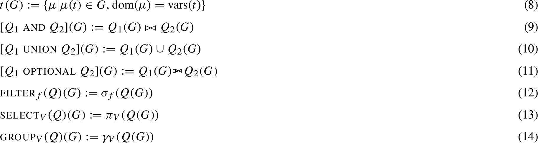
Some works have proposed extending SPARQL with similarity features. However, these works have either focused on (1) unidimensional similarity measures that consider similarity with respect to one attribute at a time [20,44], or (2) domain-specific fixed-dimensional similarity measures, such as geographic distance [1,50]. Other approaches rather pre-compute and index similarity scores as part of the RDF graphs [8,16,30] or support metric distance measures external to a query engine [29,40].
In terms of clustering, Ławrynowicz [21] proposed an extension for SPARQL 1.0 that provides the solution modifier CLUSTER BY. This modifier receives several arguments, such as the clustering algorithm and its parameters; however their proposal was not implemented and it was not updated for SPARQL 1.1 so, for instance, it is unclear how the solution modifier works with the newly added modifiers such as GROUP BY. Thus, it is still unclear how the results of a SPARQL 1.1 query should be grouped with respect to similarity criteria, rather than exact criteria, and it is unclear what the performance cost of such an operator might be.
In this paper, two operators that enrich SPARQL with similarity-based queries are presented: similarity joins and clustering. Our work is, to our knowledge, the first to consider multidimensional similarity queries in the context of SPARQL, where the closest proposal to this one is DBSimJoin [43]: a PostgreSQL extension, which – though it lacks features arguably important for the RDF/SPARQL setting, namely nearest neighbours semantics – is considered as a baseline for experiments. Our work is also pioneer on the implementation and evaluation of clustering features on top of SPARQL with read-only capabilities (other works use SPARQL Update queries for some form of clustering [37]).
Fig. 1.
Examples of queries using similarity joins and clustering in the astronomy domain.
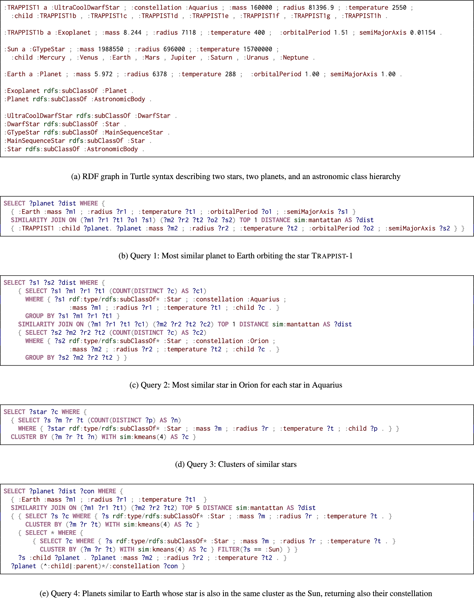
Motivating example To motivate combining similarity joins and clustering with SPARQL, we present some examples from the astronomy domain. Consider the RDF graph of Fig. 1, which describes, in Turtle syntax: the star Trappist-1, including its type, constellation, mass (ronnagrames), radius (kilometres), temperature (Kelvin), and its orbiting planets; the exoplanet Trappist-1b, including its type, mass (ronnagrames), radius (kilometres), temperature (Kelvin), orbital period (days), and semi-major axis of orbit (Astronomical Units); the Sun and the Earth, including analogous properties and units; and a class hierarchy of astronomic bodies. The example shown is based on Wikidata [45], using a fictional namespace and more readable identifiers for clarity.11 Wikidata describes millions of astronomic bodies in this way. Combining similarity joins and clustering features with the broader SPARQL 1.1 query language enables the user to pose a wide range of queries over such data. Using similarity joins, the user can find, for example:
1. The planet orbiting Trappist-1 most similar to Earth in terms of mass, radius, temperature, orbital period and semi-major axis.
2. The most similar star in the constellation Orion for each star in the constellation Aquarius, based on mass, radius, temperature and number of planets.
Using clustering, the user can find, for example:
3. Clusters of stars based on mass, radius, temperature and number of planets.
Combining both similarity joins and clustering, the user can find:
4. The top 5 most similar planets to the Earth based on their mass, radius and temperature whose stars are in the same cluster as the Sun based on mass, radius and temperature, along with each planet’s constellation.
Figure 1b–1e shows how these queries are expressed in the concrete syntax we will propose and describe in detail later in the paper. Of note is that we can use SPARQL’s other features to apply similarity joins and clustering on computed attributes of an entity; for example, the second and third queries reference the number of planets, and although this numeric attribute is not explicitly given in the data, we can compute it in SPARQL using a count aggregation. We can likewise cluster planets based on properties of their stars (e.g., their temperature), based on attributes calculated from explicit values (e.g. the density calculated from mass and radius), etc. Furthermore, we can use SPARQL’s features to retrieve additional details of results returned by similarity joins and clustering, such as the constellations of planets returned by the fourth query, retrieved via a property path.
Later we will present further examples of queries that are enabled by these features in the context of other domains, including chemistry, politics, demography, and multimedia.
Contributions This paper is an extension of our previous work, where we proposed, defined, implemented and evaluated novel types of similarity joins in SPARQL [9]. In this extended version, we discuss new use-case queries over different RDF data, and we expand the evaluation of the similarity join implementations by building a benchmark based on the query logs of Wikidata. Furthermore, we extend the proposal with a novel clustering solution modifier; we describe its syntax, semantics and implementation, and we evaluate its performance. Extended discussion and examples are also provided.
Paper outline In Section 2 we present definitions regarding RDF, the SPARQL algebra and syntax, and similarity-based operations, and in Section 3, related work. The similarity join operator, its properties, and implementation are introduced in Section 4. Section 5 is dedicated to the clustering solution modifier: its definition, a proposed syntax, the implemented clustering algorithms, and use cases. Evaluation of the similarity join operator and the clustering solution modifier is presented and discussed in Section 6. Finally, Section 7 presents our concluding remarks.
2.Preliminaries
In this section, the relevant definitions and notation that is used throughout this paper regarding RDF, SPARQL and Similarity Operations are presented.
2.1.RDF and SPARQL
RDF is the standard graph-based data model for the Semantic Web. RDF terms can be either IRIs (I), literal values (L) or blank nodes (B). An RDF triple is a tuple (s,p,o)∈IB×I×IBL,22 where s is referred to as the subject, p as the predicate, and o as the object. A finite set of RDF triples makes an RDF graph.
SPARQL is the W3C standard query language for RDF [15]. The semantics of SPARQL operators are introduced by Pérez et al. [34], in terms of their evaluation over an RDF graph. The result of the evaluation of a SPARQL query is a set of solution mappings. Let V denote a set of query variables disjoint with IBL, a solution mapping is a partial function μ:V→IBL defined for a set of variables, called its domain, dom(μ). Two solution mappings μ1, μ2 are compatible, noted as μ1∼μ2, if for all v∈dom(μ1)∩dom(μ2), μ1(v)=μ2(v). Letting X and Y denote sets of solution mappings, the SPARQL algebra is defined as follows:
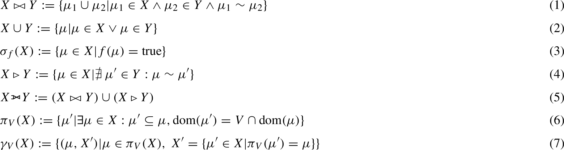
where f is a filter condition that, given a solution mapping, returns true, false, unbound or an error.
We denote the evaluation of a query Q over an RDF graph G as Q(G). Before defining Q(G), first let t=(s,p,o) denote a triple pattern, such that (s,p,o)∈VIL×VI×VIBL; then by vars(t) we denote the set of variables appearing in t and by μ(t) we denote the image of t under a solution mapping μ. Finally, we can define Q(G) recursively as follows:
2.2.Similarity search
In this section, we introduce the concept of similarity search over a universe of objects, as well as different similarity search operations.
Definition 2.1
Definition 2.1(Similarity Search).
Let U be the universe of objects, and D⊆U a dataset. Given a query object q∈U, similarity search obtains all elements x∈D such that x is similar to q.
Mathematically, similarity is modelled as a score. Let sx,y∈[0,1] be the similarity score between objects x and y, where the higher the score, the more similar x and y are. Similarity scores are often measured in terms of distances within a given space; two objects being more similar if the distance among them is small. In this work, we consider a class of distance functions called metrics:
Definition 2.2
Definition 2.2(Metric Distance).
A distance function δ:U×U→R is called a metric if the following properties hold for all x,y,z∈U:
1. δ(x,y)⩾ (positivity).
2.
3.
4.
Examples of metric distances are the Euclidean distance over real vectors, the edit distance over strings, and the Jaccard distance over sets.
Metric distances induce a topology over the set they are defined upon:
Definition 2.3
Definition 2.3(Metric Space).
A metric space is a tuple
There are two main types of similarity search queries in metric spaces: range and nearest neighbours queries.
Definition 2.4
Definition 2.4(Range Similarity Search).
Let
Definition 2.5
Definition 2.5(Nearest Neighbours Similarity Search).
Let
If instead of a single query object q we consider a set of query objects, we call this operation a similarity join. A similarity join is an operation defined over two comparable sets. Two sets are deemed comparable if a (metric) distance function can be defined over their Cartesian product.
Definition 2.6
Definition 2.6(Similarity Join).
Let
Note that similarity search – also known as query-by-example – is a special case of similarity join where
3.Related work
This section is divided in four parts: the first presents techniques to evaluate similarity joins; the second introduces works about the similarity operations available in query languages or database engines; the third is dedicated to clustering techniques; and the fourth to the inclusion of clustering in query languages.
3.1.Similarity joins
The brute force method for computing a similarity join between
A common way to optimise similarity joins is to index the data using tree structures that divide the space in different ways (offline), then pruning distant pairs of objects from comparison (online). Several tree structures have been proposed as indexes for optimising similarity queries [14,31,41]. Among such approaches, we can find vantage-point Trees (vp-Trees) [48], which make recursive ball cuts of space centred on selected points, attempting to evenly distribute objects inside and outside the ball. vp-Trees have an average-case query-by-example search time of
Other space partitioning algorithms are not used for indexing but rather for evaluating similarity joins online. The Quickjoin (QJ) algorithm [17] was designed to improve upon grid-based partition algorithms [3,5]; it divides the space into ball cuts using random data objects as pivots, splitting the data into the vectors inside and outside the ball, proceeding recursively until the groups are small enough to perform a nested loop. It keeps window partitions in the boundaries of the ball in case there are pairs needed for the result with vectors assigned to different partitions. QJ requires
Another alternative is to apply approximations to evaluate the similarity joins, trading the precision of the results for more efficient computation. FLANN [26] is a library that provides several approximate k-nn algorithms based on randomised k-d-forests, k-means trees, locality-sensitive hashing, etc.; it automatically selects the best algorithm to index based, for example, on a target precision, which can be traded-off to improve execution time.
3.2.Similarity in databases
Though similarity joins do not form part of standard query languages, such as SQL or SPARQL, a number of systems have integrated variations of such joins within databases. In the context of SQL, DBSimJoin [43] implements a range-based similarity join operator for PostgreSQL. This implementation claims to handle any metric space, thus supporting various metric distances; it is based on the aforementioned index-free Quickjoin algorithm.
In the more specific context of the Semantic Web, a number of works have proposed online computation of similarity joins in the context of domain-specific measures. Zhai et. al [50] use OWL to describe the spatial information of a map of a Chinese city, enabling geospatial SPARQL queries that include the computation of distances between places. The Parliament SPARQL engine [1] implements an OGC standard called GeoSPARQL, which aside from various geometric operators, also includes geospatial distance. Works on link discovery may also consider specific forms of similarity measures [40], often string similarity measures over labels and descriptions [44].
Other approaches pre-materialise distance values that can then be incorporated into SPARQL queries. IMGpedia [8] pre-computes a k-nn self-similarity join offline over images and stores the results as part of the graph. Similarity measures have also been investigated for the purposes of SPARQL query relaxation, whereby, in cases where a precise query returns no or few results, relaxation finds queries returning similar results to those sought [16,30].
Galvin et al. [10] propose a multiway similarity join operator for RDF; however, the notion of similarity considered is based on semantic similarity that tries to match different terms referring to the same real-world entity. Closer to this work lies iSPARQL [20], which extends SPARQL with IMPRECISE clauses that can include similarity joins on individual attributes. A variety of distance measures are proposed for individual dimensions/attributes, along with aggregators for combining dimensions. However, in terms of evaluation, distances are computed in an attribute-at-a-time manner and input into an aggregator. For the multidimensional setting, a (brute-force) nested loop needs to be performed; the authors leave optimisations in the multidimensional setting for future work [20].
3.3.Clustering
Clustering is a process through which a set of objects can be automatically partitioned into groups – called clusters – such that the distance between objects of a cluster is minimised, and the distance between objects in different clusters is maximised. Clustering algorithms can be roughly divided into distance-based, density-based, grid-based, distribution-based, and can also be hierarchical. A prime example of distance-based clustering algorithms is k-means [24], which first randomly selects k centroids and assigns each object to the cluster defined by the closest centroid; it then recomputes new centroids as the mean objects of each current cluster (which may not be a part of the set of objects), and reassigns the objects to the clusters defined by these new centroids until the centroids converge. The k-medoids algorithm is similar to k-means [19], but instead of centroids, it defines medoids: the element of a cluster such that its distance to every other element in the cluster is minimal. As for density-based algorithms, DBSCAN [7] groups together objects in dense regions (every object has several neighbours), separated by low density, sparse regions. DBSCAN also marks isolated objects as outliers, which are not included in any cluster. Grid-based methods, such as STING [46] and GriDBSCAN [25] divide the space into cells, aiming to quickly find dense areas to produce the clusters, and prune sparse areas as noise. However, these methods have been proven to not scale well with increasing dimensions [53]. Distribution-based methods assume that objects in the same cluster have a similar probability distribution: DBCLASD [47] assumes that the points inside a cluster are uniformly distributed. Finally, hierarchy-based approaches generate clusters within clusters forming a hierarchy that can be consumed at various levels. Hierarchical clustering methods include BIRCH [52], CURE [13], and Chameleon [18].
3.4.Clustering in databases
In databases, Ordonez and Omiecinski [32] provide an efficient disk-based k-means implementation for RDBMS using SQL INSERT and UPDATE queries. Also in SQL, Zhang and Huang [51] propose to extend the query language with a CLUSTER BY keyword, however, they do not provide an implementation. Li et al. [22] propose to extend SQL with fuzzy criteria for grouping and ordering, which they call clustering and ranking; they provide syntax and semantics, as well as a C
Qi et al. [37] provide a k-means implementation for RDF data by using SPARQL Update queries. Ławrynowicz [21], proposed an extension to SPARQL 1.0, that introduces a CLUSTER BY solution modifier along with a clear syntax and semantics; however, they do not include an implementation nor evaluation, and it is not immediately clear how their proposal could be aligned with SPARQL 1.1 grouping and aggregates.
4.Similarity joins in SPARQL
In this section, the similarity join operator for SPARQL is presented. Along with the algebraic definition of the operator and its properties, we will present options for its implementation and optimisation, and further introduce use-case queries to illustrate its application. We first define the following general criteria that a novel similarity join operator for SPARQL 1.1 should satisfy:
Closure: | the new operator should be freely combinable with other available operators. |
Extensibility: | the similarity join should allow the user to specify the required dimensions and metrics to be used in the query, and define new metrics as needed. |
Robustness: | the new operator should make as few assumptions as possible about the input or the data, regarding completeness, comparability, etc. |
Usability: | the new operator should be easy for users to adopt, offering high expressiveness while avoiding unnecessary verbosity. |
With respect to Closure, the similarity join will be defined in a manner analogous to other forms of joins that combine graph patterns in the WHERE clause of a SPARQL query; furthermore, the computed distance measure is allowed to be bound to a variable, facilitating its use beyond the similarity join (e.g., for solution modifiers such as ORDER BY, for aggregates such as MAX, MIN, AVG, for expressions within FILTER or BIND, etc). With respect to Extensibility, rather than assume one metric, the type of distance metric used is explicit in the semantics and syntax, allowing other types of distance metrics to be used in future. Regarding Robustness, the precedent of SPARQL’s error-handling when dealing with incompatible types or unbound values is followed. Finally, regarding Usability, syntactic features for both range-based similarity joins and k-nn similarity joins are supported, noting that specifying particular distances for ranges can be unintuitive in abstract, high-dimensional metric spaces.
4.1.Syntax
To define the syntax for a similarity join, it is necessary to consider the syntax of other binary operators such as OPTIONAL or MINUS [15], as well as the required extra parameters: the variables representing the dimensions with respect to which the distance is to be computed, the distance function to be used, a fresh variable to bind the computed distances to, and the similarity parameter corresponding to a threshold distance (for range similarity joins) or to a threshold number of nearest neighbours (for k-nn similarity joins).
The syntax for the similarity join operator extends the SPARQL 1.1 EBNF grammar [15] by adding one production rule for SimilarityGraphPattern, and extending the rule for GraphPatternNotTriples. All other definitions are left unchanged. The exact changes to the grammar can be found in Fig. 2.
Fig. 2.
The extended production rules from SPARQL 1.1 to support similarity joins.

The keyword ON is used to define the variables in both graph patterns upon which the distance is computed; the keywords TOP and WITHIN denote a k-nn query and an r-range query respectively; the keyword DISTANCE specifies the IRI of the distance function to be used for the evaluation of the join, whose result will be bound to the variable indicated with AS, which is expected to be fresh, i.e., to not appear elsewhere in the SimilarityGraphPattern, similarly to BIND. The syntax may be extended in the future to provide further customisation, such as supporting different normalisation functions, or to define default parameters.
Depending on the metric, it could be possible, in principle, to express such queries as plain SPARQL 1.1 queries, by taking advantage of features such as variable binding, numeric expressions, sub-selects, etc. However, there are two key advantages of the dedicated syntax: (1) similarity join queries in vanilla syntax would be complex to express, particularly in the case of k-nn queries or metrics without the corresponding numeric operators in SPARQL; (2) optimising queries written in the vanilla syntax (beyond nested-loop performance) would be practically infeasible, requiring an engine that can prove equivalence between the distance metrics and semantics for which similarity join algorithms are optimised and the plethora of ways in which they can be expressed in vanilla syntax. This is why we propose to make similarity joins for multidimensional distances a first class feature, with dedicated syntax and physical operators offering sub-quadratic performance in average/typical cases.
4.2.Semantics
We now introduce some definitions to extend the SPARQL semantics defined in Section 2 to cover the similarity joins whose syntax is defined in Section 4.1. These definitions adapt the standard definitions of similarity joins as presented in Section 2.2 to make them compatible with the relational algebra underlying SPARQL, i.e., to perform an equi-join on shared variables, and a similarity join on other variables selected by the user.
We start with the definition of a similarity join expression, which indicates the criteria under which the similarity of two SPARQL solution mappings can be computed.
Definition 4.1
Definition 4.1(Similarity Join Expression).
A similarity join expression is a 4-tuple
In the following, we present several definitions that build up to the formal specification of our similarity join operators. We begin with a definition that, given two compatible solutions from either side of the similarity join
Definition 4.2.
Given two compatible solution mappings
Note that per this definition,
Next we define some useful notation for the result of a natural equi-join (applying a join with equality on shared variables, i.e., based on compatible solutions) that forms the basis of our similarity join operator.
We denote by
Given a set of solutions, we now define notation for the union and intersection of the domains of the solutions (the sets of variables for which a solution is defined).
Definition 4.3.
Given a set of solution mappings X we define the union and intersection domains as:
In order words,
The next definition allows us to define a solution mapping that maps specific variables to specific SPARQL terms (similar to BIND). This will be used to bind the distance value to a specified (fresh) variable.
Definition 4.4.
Letting
With all these definitions in hand, we introduce the similarity join operators in SPARQL as follows:
Definition 4.5
Definition 4.5(Range Similarity Joins in SPARQL).
Given two sets of solution mappings X and Y and a similarity join expression
Definition 4.6
Definition 4.6(k-nn Similarity Joins in SPARQL).
Given two sets of solution mappings X and Y and a similarity join expression
Per Definition 4.6, more than k results can be returned for
An error is returned when
Bag semantics are defined for similarity joins in the natural way, where the multiplicity of
Next, given the semantics of the similarity join operators, we present several algebraic properties for the similarity join and its relationship with other SPARQL operators. These properties and equivalences are useful for query planning and optimisation. For instance, having a commutative and associative operator can allow the Query Planner to choose the best possible order in which to evaluate a given sequence of these operators; similarly, having equivalences between operators under certain circumstances can allow for query rewriting and further optimisation. Particularly for the case of similarity joins, some rewriting rules can help to reduce the sets of intermediate solutions considerably before applying the similarity join, and thus reduce query execution time. The proofs for each of the claims along with some illustrative examples can be found in the Appendix:
1.
2.
3.
4.
5. Let
(a)
(b)
(c)

(d)
A key finding here is that properties that hold for (equi) joins in SPARQL do not necessarily hold for similarity joins (commutativity, associativity, distributivity), and these equivalences show how and why this is the case. This means that common optimisations applied in SPARQL engines (such as join reordering) cannot be applied as is for similarity joins, and thus there are interesting open challenges on how to optimise these queries.
4.3.Implementation
The implementation of the similarity join operators extends ARQ – the SPARQL engine of Apache Jena33 – which indexes an RDF dataset and receives as input a (similarity) query in the syntax discussed in Section 4.1. The steps of the evaluation of an extended SPARQL query follow a standard flow, namely Parsing, Algebra Optimisation, Algebra Execution, and Result Iteration. The implementation is available at https://github.com/scferrada/jena.
The Parsing stage receives the query string written by a user, and outputs the algebraic representation of the similarity query. Parsing is implemented by extending the Parser of Jena using JavaCC,44 wherein the new keywords and syntax rules are defined, as introduced in Section 4.1. The result of the Parsing stage is an abstract syntax tree of algebraic operators, e.g., knnsimjoin(leftjoin(…), triplepattern(…)).
In terms of physical operators to evaluate the similarity joins, initially we considered applying offline indexing of literal values in the RDF graph in order to allow lookups of similar values. However, we discarded this option for the following two reasons:
– Indexing approaches typically consider a fixed metric space, with a fixed set of attributes specified for the distance measure (e.g., longitude and latitude). Conversely, in our scenario, the user can choose the attributes according to which similarity will be computed for a given query. In the setting of an RDF graph such as DBpedia or Wikidata, the user can choose from thousands of attributes. Indexing all possible combinations would lead to an exponential blow-up and would be prohibitively costly in terms of both time and space.
– Aside from selecting explicit attributes in the data – and per the Closure requirement – the user may often wish to compute attributes upon which distance can be measured. For example, when comparing countries, the user may wish to use the number of cities in each country (computed with COUNT), or the GDP per capita (dividing the GDP by the population). It would not be feasible to pre-index these computed attributes.
For this reason, we rather consider online physical operators that receive two sets of solution mappings and compute the similarity join. Some of these physical operators include indexing techniques, but these indexes are built online – for a specific query – over intermediate solutions rather than the RDF graph itself.
The similarity join physical operators apply a normalisation function to each of the dimensions of the space, in order to avoid differences in scale of these dimensions to affect disproportionately the similarity of two solution mappings. For example, a similarity join query computing distances w.r.t. the dimensions human development index, HDI, (a number in
Algebra Optimisation then applies static rewriting rules over the query, further turning logical operators (e.g., knnsimjoin) into physical operators. In terms of the physical operators, we implement three variants:
Nested Loops | involves a brute-force pairwise comparison, incurring quadratic cost for similarity joins. It computes exact results for both range and k-nn queries and is intended as a performance baseline. |
vp-Trees | is an index-based approach based on applying ball-cuts in the metric space. It computes exact results for both range and k-nn queries. Though the worst-case for similarity joins is still quadratic, depending on the distance distribution, dimensionality, etc., vp-Trees can approach linear performance. |
FLANN | is an ensemble of approximate methods for k-nn queries only, where the best approach is chosen based on the query, data, target precision, etc. |
Algebra Execution begins to evaluate the physical operators chosen in the previous step, with low-level triple/quad patterns and path expression operators feeding higher-level operators. Finally, Result Iteration streams the final results from the evaluation of the top-level physical operator. All physical similarity-join operators follow the same lazy evaluation strategy used for the existing join operators in Jena.
Besides the implementation of sub-quadratic average-case similarity join physical operators, there are other avenues for query optimisation, namely: query rewriting and result caching. As for rewriting rules, there is little opportunity for applying such rules because of a) similarity joins are a relatively expensive operation to compute, thus the best option is to reduce the size of the outputs of the sub-operands as early as possible and therefore, making typical rewriting rules impractical (such as delaying filters and optionals); and b) we see in Section 4.2 that the k-nn similarity join operator is not commutative nor associative, further preventing rewriting such as join reordering.
4.4.Use-case queries
Back in Section 1, we presented some motivating example queries that can be written using our proposed extension to SPARQL over a small artificial dataset. Now, in this section, we present three use-case queries demonstrating different capabilities of the extension, which are based on real-world data from Wikidata [45] and IMGpedia [8]. All prefixes used in the queries of this paper are listed in Table 1.
Table 1
IRI prefixes used in the paper
| Prefix | IRI |
| wdt: | ⟨http://www.wikidata.org/prop/direct/⟩ |
| wd: | ⟨http://www.wikidata.org/entity/⟩ |
| sim: | ⟨http://sj.dcc.uchile.cl/sim#⟩ |
| imo: | ⟨http://imgpedia.dcc.uchile.cl/ontology#⟩ |
| tdb: | ⟨https://triplydb.com/triply/iris/def/measure/⟩ |
| stp: | ⟨http://stars.dcc.uchile.cl/prop/⟩ |
| dbo: | ⟨http://dbpedia.org/ontology/⟩ |
| nobel: | ⟨http://data.nobelprize.org/terms/⟩ |
| country: | ⟨http://data.nobelprize.org/resource/country/⟩ |
Fig. 3.
Query for non-metal chemical elements similar to metallic elements in terms of atomic properties.
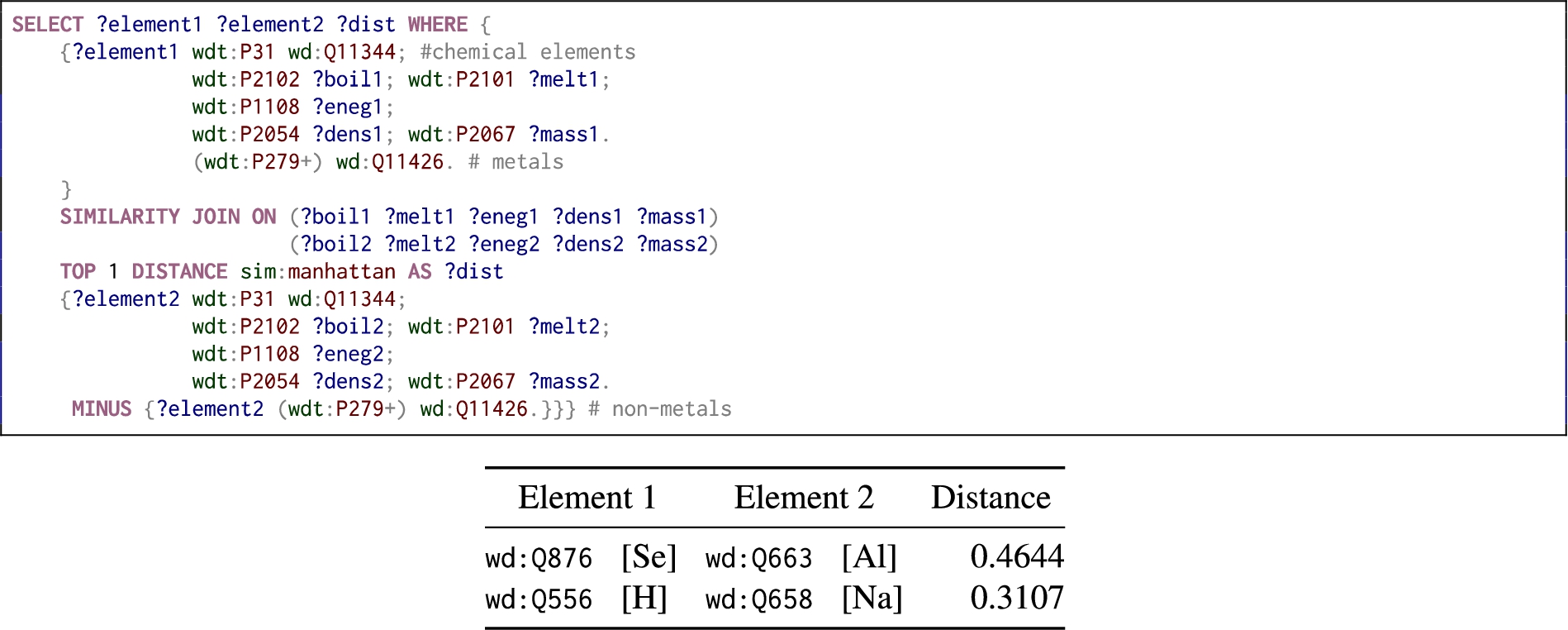
Similar chemicals Chemical elements contain several numeric/ordinal properties, such as boiling and melting point, mass, electronegativity and so on. In Fig. 3 we request for metals similar to non-metals in terms of those properties, along with sample results of the similar metal/non-metal query. Figure 3 also presents a selection of results of the query, where we see that Selenium is most similar to Aluminium, and Hydrogen to Sodium.
Fig. 4.
Query requesting countries that have a number of Literature, Chemistry, Physics and Medicine Nobel Prizes similar to those of Canada.
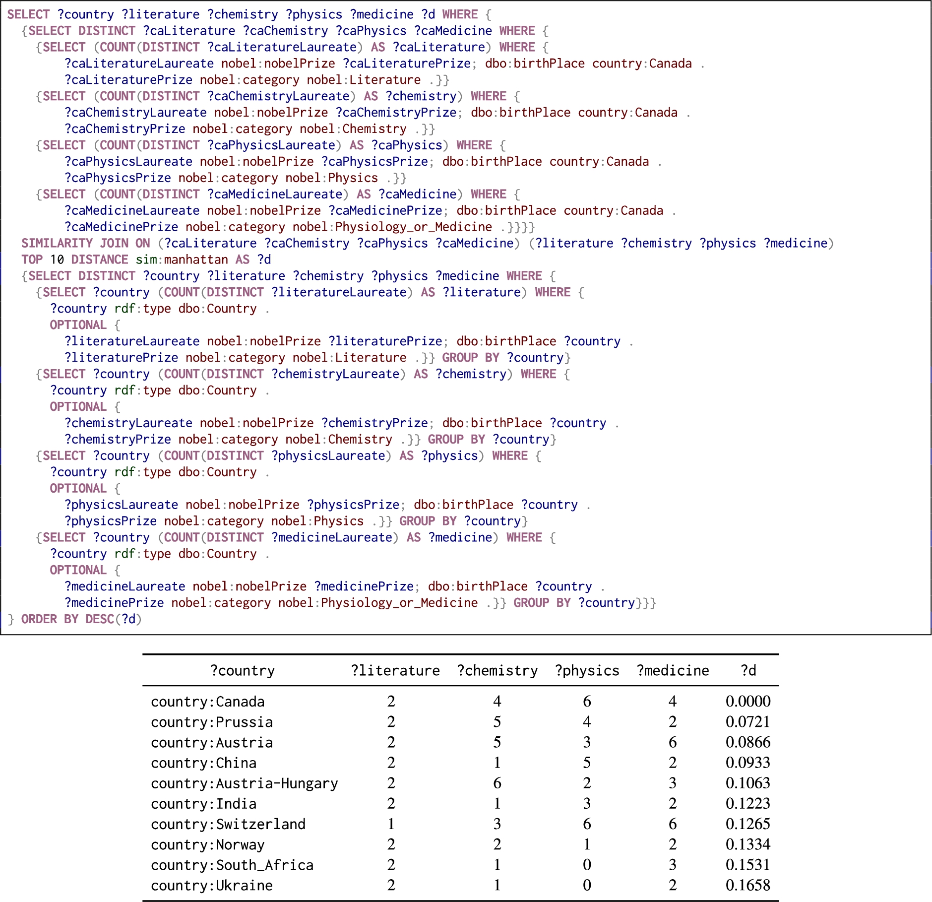
Similar laureates: Figure 4, presents a more complex similarity query over the Nobel Prize Linked Dataset55 to find the 10 countries that have the most similar number of Nobel Prize laureates in literature, chemistry, physics and medicine than Canada. Figure 4 also presents the query results.
Fig. 5.
Query for the 10 images of towers most similar to each image of the Entel Tower in terms of the HOG visual descriptor.
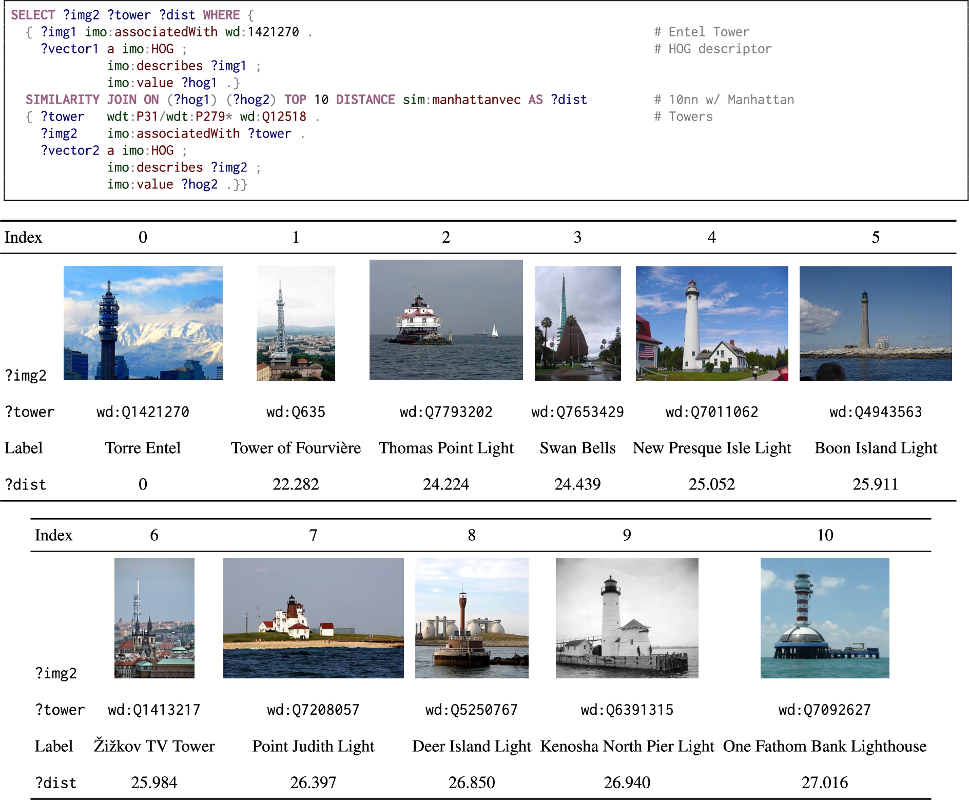
Similar images: Figure 5 presents a similarity query over IMGpedia [8]: a multimedia Linked Dataset. The query retrieves images of the Entel Tower in Chile, and computes a 10-nn similarity join for images of towers based on a precomputed Histogram of Oriented Gradients (HOG) descriptor, which extracts the distribution of edge directions of an image. Note that this query uses a different distance funtion IRI than the previous two, since variables ?hog1 and ?hog2 are bound to string serializations of vectors, and thus the function sim:manhattanvec deals with the parsing of such strings as well. The figure includes a sample of the results for one of the images of the Entel Tower (in index 0), showing for each similar image, the related Wikidata entity, its label, and the distance to the source image.
5.Clustering solution modifier
In this section, we analyse, implement and evaluate a CLUSTER BY solution modifier for SPARQL queries – inspired by the proposal of Ławrynowicz [21] – based on the aforementioned notions of similarity and distance. First, we discuss how this extension of SPARQL was initially conceived, how it can be formalised syntactically and semantically and how it interacts with the rest of the solution modifiers. We then discuss implementation details for the solution modifier, and present a prototype built on top of Apache Jena. Finally, use-case queries are presented.
As it has been argued before in this paper, users sometimes require non-exact matches over the data and instead wish for similar matches. This is also the case when using the solution modifier GROUP BY in SPARQL, which makes a partition of the resulting mappings of a query based on certain variable values that need to match exactly in order to assign a binding into a group. In SPARQL 1.1 [15] the algebra of GROUP BY is defined as described in Section 2.
As presented, the GROUP BY modifier partitions the bindings into equivalence classes (the
5.1.Syntax
In order to support clustering in SPARQL, we must first define its syntax and semantics in a way that a user can express the clustering variables, and the algorithms and their required parameters. Ławrynowicz [21] proposes the following extension for SPARQL 1.0 [36], where the cluster identifier is bound AS a fresh variable (cf. Fig. 6).
![Syntactic extension to the SPARQL 1.0 grammar for clustering [21].](https://content.iospress.com:443/media/sw/2024/15-5/sw-15-5-sw243540/sw-15-sw243540-g007.jpg)
The first thing that can be noticed from the definition is that, since the extension was conceived for SPARQL 1.0, it lacks the definition of the GROUP BY solution modifier. The definition of a clustering solution modifier for SPARQL 1.1 needs to take into account the existence of GROUP BY, and how it shall interact with CLUSTER BY.
Since clustering is the similarity-based version of grouping (which is based on exact matching), one alternative is to make the modifiers CLUSTER BY and GROUP BY be mutually exclusive in a query. However, the two modifiers can be made compatible by defining the clustering modifier as binding the cluster identifier of each mapping to a fresh variable, potentially allowing users to later group the results by the identifier value; in other words, CLUSTER BY extends the solution mappings with an extra variable bound to a cluster identifier, rather than directly grouping them. This decision is made since any new operation included into a query language should be as non-disruptive as possible, and to preclude the usage of GROUP BY when clustering is indeed disruptive.
Since the CLUSTER BY solution modifier is not mutually exclusive with GROUP BY, CLUSTER BY does not interact with the HAVING clause and the different aggregators, which can rather be computed after the clustering takes place. Conversely, in order to apply clustering with respect to values computed through aggregation functions, the aggregation must be computed in a subquery. Thus, following the SPARQL spec, the order of the solution modifiers including CLUSTER BY is: clustering, grouping, having, ordering, projection, distinct, reduced, offset, and limit.
Ławrynowicz [21] makes use of the SPARQL Query Results Clustering Ontology (SQRCO) to define the clustering algorithm and its parameters as a set of triples in the query. However, at the time of writing, the ontology is not found on the Web and is not registered in prefix.cc. We instead take a syntax-based approach, using special keywords for the clustering configuration, similarly to what is done with the similarity join operator.
Our proposed extension of the SPARQL 1.1 syntax that includes CLUSTER BY is presented in Fig. 7. The extension adds a new production rule, ClusterByClause, as an alternative in the SolutionModifier production rule. We make use of the Extension Function framework defined for SPARQL 1.1 to allow users to define the desired clustering algorithm and its parameters by using an iriOrFunction rule after the keyword WITH, thus allowing the function to be called without any parameters as well, which permits to define default values for each supported algorithm. Finally, we provide syntax to define the fresh variable on which the cluster identifier shall be bound AS. We permit only variables to be used as clustering attributes, but expressions could be supported in a future version. Nevertheless, expressions could be indirectly used for clustering by using the BIND function.
Fig. 7.
Syntactic extension to the SPARQL 1.1 grammar for clustering.

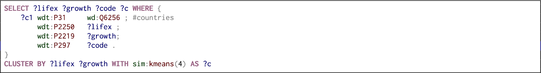
An example of a SPARQL query that uses this extension can be appreciated in Fig. 8, where the countries available in Wikidata are clustered based on their life expectancy and economic growth. The query specifies that the clustering shall use k-means returning 4 clusters. Notice that we also obtain the 2-letter ISO code for each country (property wdt:P297) and we are able to project that variable even if it is not part of the CLUSTER BY variables.
Fig. 8.
Example SPARQL query with the CLUSTER BY solution modifier.
5.2.Semantics
Given the SPARQL semantics presented in Section 2, as well as the discussed syntax for CLUSTER BY, we now propose the semantics for the CLUSTER BY solution modifier, per the following definition.
Definition 5.1.
Given a multiset of solution mappings X, the clustering algorithm
5.3.Implementation
Analogous to the similarity join operators, we implement the CLUSTER BY solution modifier on top of Apache Jena’s ARQ, where the code is publicly available in the following repository: https://github.com/scferrada/jena. The implementation supports three clustering algorithms: k-means, k-medoids, and DBSCAN. These algorithms are currently implemented in-memory. All three algorithms use the Manhattan distance as the dissimilarity measure. All three algorithms enumerate the clusters in no particular order using natural numbers starting from 1, and use said numbers as the identifiers of the clusters. For k-medoids we implemented the FastPAM1 algorithm proposed by Schubert and Rousseeuw [38] which is
Each algorithm requires different parameters, but the implementation offers default values for them, if the user does not wish to specify them. The parameters of each algorithm and the chosen default values are:
– k-means [24]: k, the number of clusters to be returned, default 3; m, the number of iterations to terminate the algorithm, default 10.
– k-medoids [19]: k, the number of clusters to be returned, default 3.
– DBSCAN [7]: ε, the distance to search for neighbours of an object, default 0; p, the minimum number of neighbours that an object needs to be considered part of a cluster, default 1.
DBSCAN is different from k-means and k-medoids in that it does not require the number of clusters to be specified, but also may mark some objects as outliers, not being in any cluster. To comply with the semantics of CLUSTER BY, it assigns all solution mappings marked as outliers to a special cluster (with identifier
Other clustering algorithms were not chosen for various reasons: both grid-based and distribution-based methods do not scale well when dimension increases [53]. Hierarchical clustering methods are left for future versions, because given the syntax and semantics of the clustering solution modifier, it would be hard to add multiple variables bound to different levels of clustering. An initial option to support these methods would be to force the user to choose a clustering level to retrieve, but we argue that in most cases, the user might not know which level of clustering is most significant for their purposes.
5.4.Use-cases
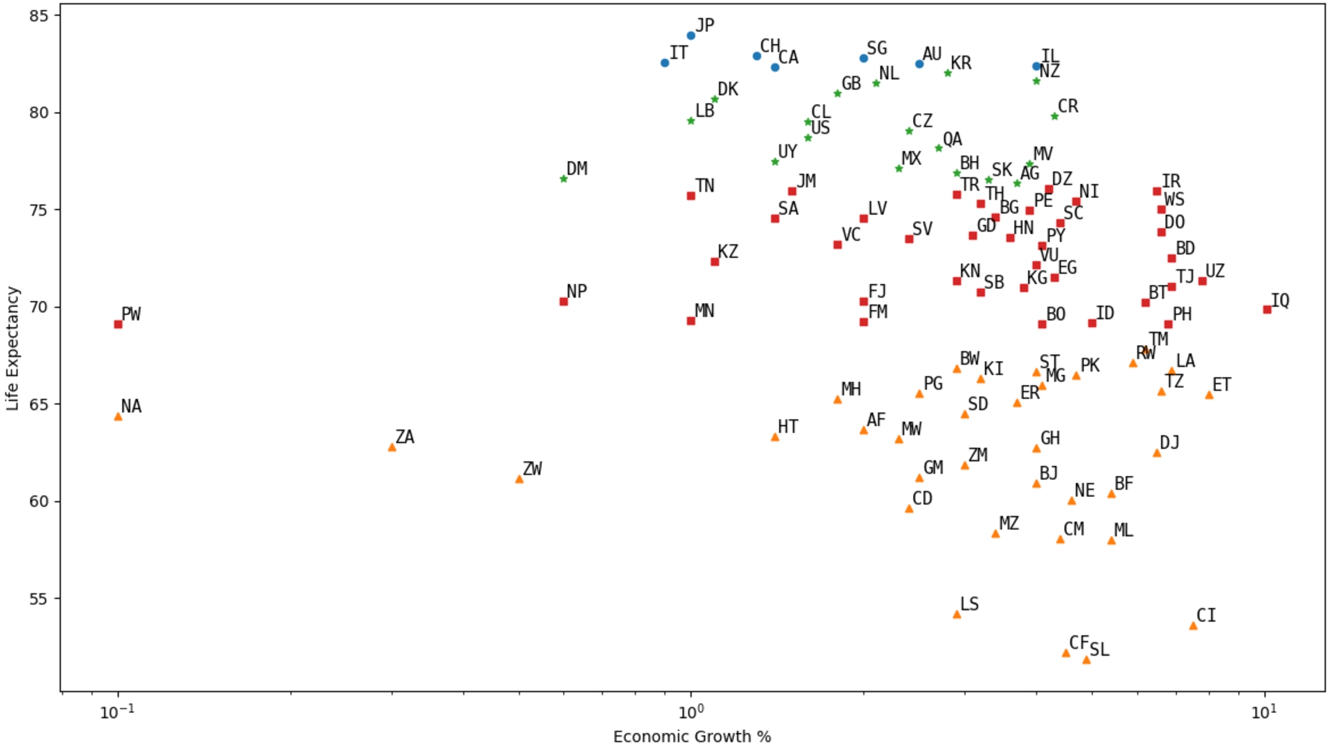
Expanding on the motivating example queries of Section 1 (see Fig. 1d–1e), we now showcase three queries that use the clustering solution modifier here proposed in different domains. First, in Fig. 9 we display the result of the query presented in Fig. 8, that clusters the countries in Wikidata with respect to their life expectancy and economic growth rate. Some results were omitted to avoid clutter in the figure. Each point has a different colour and marker depending on their assigned cluster (whose identifier is bound to variable ?c). It can be seen in this case that, since there are differences in the magnitudes of the values of life expectancy and economic growth rate, the largest values tend to weigh more in the distance value and thus, in this example, we see a stronger division along the vertical axis. To prevent that any given dimension has a disproportionate influence over the distance function, it is recommended to normalise each dimension before clustering. Additionally, we note that, unlike GROUP BY, we can keep and project any variables that are not part of the CLUSTER BY clause. In Fig. 9 we also present the 2-letter ISO code of each country (which is directly obtained from the query) annotating each point in the graph, so that the reader can know which countries belong to each cluster more easily.
Fig. 9.
Clusters of countries by growth and life expectancy.
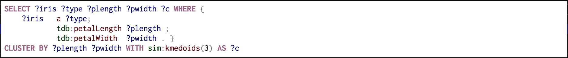
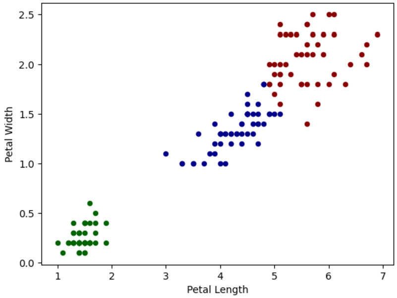
Then, the Iris Dataset in RDF66 is used to run a clustering query on petal length and width. In Fig. 10 the extended SPARQL query that divides the objects into three clusters using the k-medoids algorithm is presented. Figure 11 shows the results of the clustering, where the green cluster is iris setosa, the blue cluster is mostly iris virginica, and the red cluster is mostly iris versicolor. Notice that the iris types can also be retrieved with the query.
Fig. 10.
Extended SPARQL query to obtain three clusters of iris.
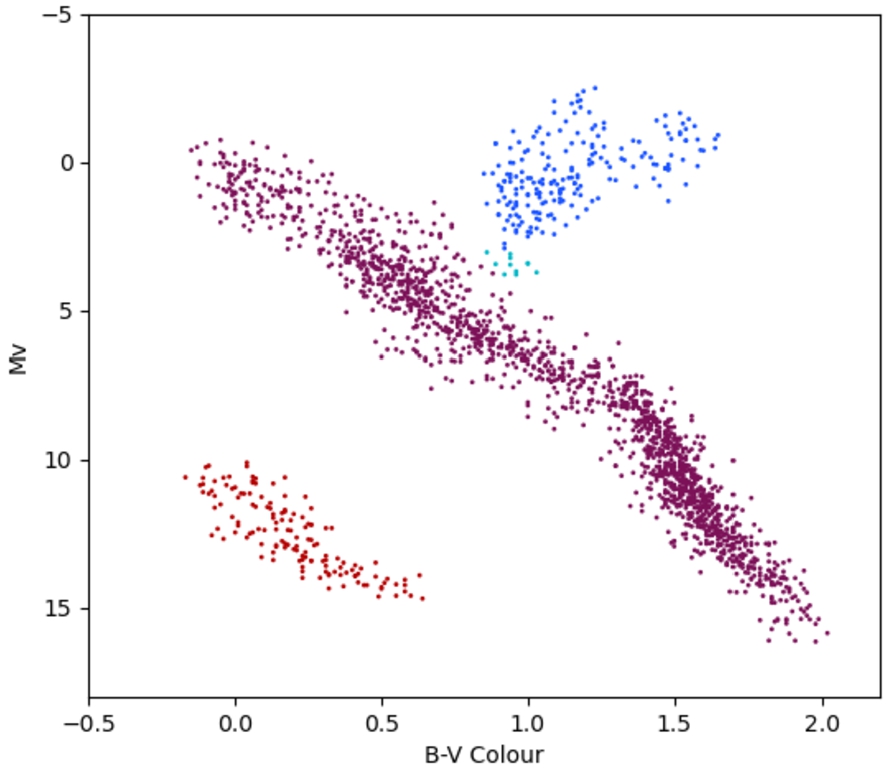
Next, we present a Hertzsprung–Russell (HR) diagram, that is used in astronomy to classify stars into main sequence, giants, white dwarfs, etc. HR diagrams have the normalised B–V Colour (a measure of the temperature or “brightness” of the star) on the X-axis, and
Fig. 12.
Extract of the RDF data for stars.

Fig. 13.
SPARQL query for clustering star data.
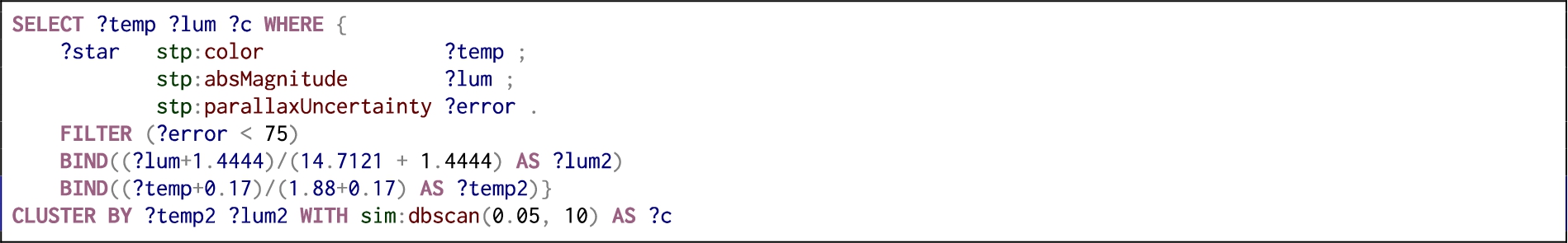
Fig. 14.
Visual representation of the star clusters obtained with query from Fig. 13. Outliers not presented.
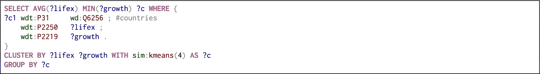
Finally, we showcase how the CLUSTER BY solution modifier can interact with GROUP BY in a SPARQL query. To do this, we modify the query from Fig. 8, which obtains the life expectancy and growth rate of the countries in Wikidata, to now GROUP BY cluster identifier and compute the average life expectancy and the minimum growth rate of each cluster. This query is presented in Fig. 15, and the results of its evaluation over Wikidata can be seen in Table 2 where cluster 1 corresponds to the dark blue cluster in Fig. 9, which includes Japan and Italy, and has the highest life expectancy and a minimum growth rate of 0.9%; cluster 2 is the pink cluster, which contains New Zealand and Chile; cluster 3 is the sky blue cluster, which includes Brazil and Bulgaria, and presenting the lowest growth rate at −18%; and cluster 4 is the red cluster, presenting the lowest life expectancy average.
Fig. 15.
Example SPARQL query with the CLUSTER BY solution modifier and GROUP BY.
6.Experimental results
Experimental results for both the similarity join operator and the clustering solution modifier are presented in this section. Unless stated otherwise, experiments were run on a machine with Ubuntu 20, an 8-core Intel® CoreTM i7-6700 CPU @3.4 GHz, 16 GB of RAM and a 931 GB HDD. We provide the experiment code, queries, etc., online.88
Table 2
Results of query of Fig. 15
| ?c | AVG(?lifex) | MIN(?growth) |
| 1 | 83.399 | −5.42 |
| 2 | 78.696 | −3.20 |
| 3 | 73.121 | −18.00 |
| 4 | 61.909 | −13.80 |
6.1.Similarity join evaluation
We compare the performance of different physical operators for similarity joins in the context of increasingly complex SPARQL queries, as well as a comparison with the baseline system DBSimJoin. We conduct experiments with respect to two benchmarks: the first is a benchmark we propose for Wikidata, while the second is an existing benchmark used by DBSimJoin based on visual descriptors of images.
6.1.1.Wikidata: k-nn self-similarity queries
Extending the performance experimentation presented in our previous work [9], we now present similar experiments using real SPARQL queries. We use a truthy version of the Wikidata RDF dump.99 We start with SPARQL queries from the Wikidata query logs, and apply several filters: first, at least one numeric attribute must be projected in the SELECT clause; second, these numeric attributes must not be obtained in an OPTIONAL clause; third, they produce at least 8 solution mappings; and fourth, they are executed in less than 3 hours using Jena. We obtain 2,726 SPARQL queries. For each of these base queries, we wrote a k-nn self-similarity join version for our experiments.
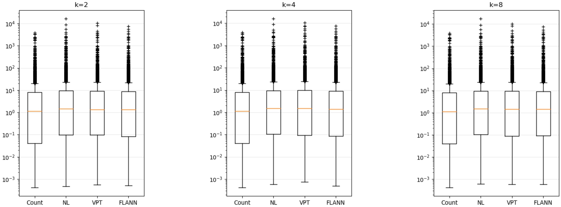
We executed self-similarity joins with
Fig. 16.
Execution time for self-similarity join queries, for different values of k.
6.1.2.Corel colour moments: Range similarity queries
The system proposed in this work is compared with the closest found in literature, DBSimJoin [43], a PostgreSQL extension that supports range-based similarity joins in metric spaces implementing the Quickjoin (QJ) algorithm. As DBSimJoin only supports range queries, it is to be compared with the vp-Tree implementation in Jena (Jena-vp). The DBSimJoin system was originally tested with synthetic datasets and with the Corel Colour Moments (CCM) dataset, which consists of 68,040 records of images, each described with 9 dimensions representing the mean, standard deviation and skewness for the colours (red, green and blue) of the pixels of the image. For CCM, the DBSimJoin paper only reports the effect of the number of QJ pivots on the execution time when
To find suitable distances, we first compute a 1-nn self-similarity join, where we take the maximum 1-nn distance in the result: 5.9; this distance ensures that each object has at least one neighbour in a range-based query with
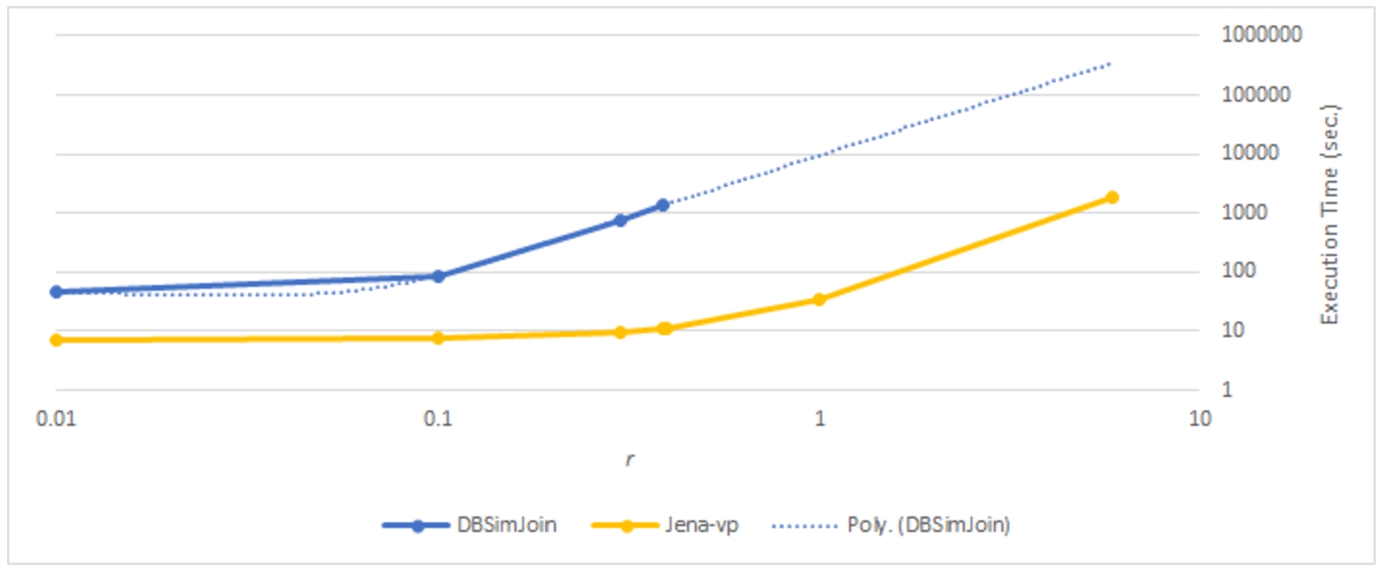
DBSimJoin is implemented and distributed an extension for PostgreSQL 8. When installed in the current hardware, it crashed with any similarity join query, because of the use of outdated I/O directives, making it impossible to re-run the experiments. Thus, we present the results previously reported [9] where we compare them with Jena-vp using the same dataset, the same queries, and the same hardware reported in [9]. Here, we provide extended discussion over these results, which are presented in Table 3. The execution time of DBSimJoin grows rapidly with r because of the quick growth of the size and number of window partitions in the QJ algorithm. DBSimJoin crashes with
Considering range-based similarity joins, these results indicate that Jena-vp outperforms DBSimJoin in terms of efficiency (our implementation is faster) and scalability (our implementation can handle larger amounts of results).
Table 3
Execution times in seconds for range similarity joins over the CCM dataset
| Distance | # of Results | DBSimJoin (s) | Jena-vp (s) |
| 0.01 | 68,462 | 47.22 | 6.92 |
| 0.1 | 68,498 | 84.00 | 7.45 |
| 0.3 | 72,920 | 775.96 | 9.63 |
| 0.39 | 92,444 | 1,341.86 | 11.17 |
| 0.4 | 121,826 | – | 11.30 |
| 1.0 | 4,233,806 | – | 35.01 |
| 5.9 | 395,543,225 | – | 1,867.86 |
Fig. 17.
Execution time of range-based self-similarity joins, including polynomial trend line for DBSimJoin times beyond
6.2.Clustering experimental results
To gain insight on the performance of the clustering solution modifier, we measure the overhead produced by the clustering algorithms. To achieve this, we prepared 1,000 synthetic SPARQL queries that draw values from the numeric properties of Wikidata. The queries are composed of only one Basic Graph Pattern (BGP), and we apply clustering over its solutions. To produce these queries, we begin with some data exploration. Specifically, from a Wikidata dump, we compute the ordinal/numeric characteristic sets [28] by: (1) filtering triples with properties that do not take numeric datatype values, or that take non-ordinal numeric datatype values (e.g., Universal Identifiers); (2) extracting the characteristic sets of the graph [28] along with their cardinalities, where, specifically, for each subject in the resulting graph, we extract the set of properties for which it is defined, and for each such set, we compute for how many subjects it is defined. Finally, we generate CLUSTER BY queries from 1,000 ordinal/numeric characteristic sets containing more than 3 properties that were defined for at least 500 subjects.
Then, we execute these queries with different parameters, in order to compare the execution time of the three implemented algorithms under various realistic configurations. These parameters are:
– For k-means:
– For DBSCAN:
– For k-medoids:
We use as a baseline the execution time of the query that COUNTs the results of the underlying BGP of each benchmark query, so as to measure the overhead produced by the CLUSTER BY operators.
Fig. 18.
Execution time of the CLUSTER BY queries using k-means clustering.
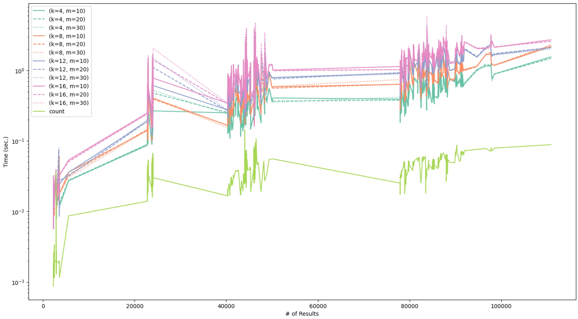
In Fig. 18, we present the results for the queries using the k-means algorithm. We use same-coloured lines for runs with the same value of k, and different dashing for different values of m. The baseline is shown with the light green line. We observe that the execution time increases as the value of k and n increases, and that the value of m does not significantly influence the execution time. This is expected, since k-means has an upper bound time complexity of
The results for the queries using DBSCAN are harder to interpret, as the execution time also depends on the distance distribution of the space defined by the solution mappings obtained from evaluating each BGP. This is because DBSCAN’s cost depends on the cost of performing ε-range searches, and on the number of found neighbours. This can be noticed in Fig. 19, which presents a plot where queries with the same value for ε are shown in the same colour, and queries with the same value for p are shown with the same line dashing. The baseline is shown with the light green line. In Fig. 19, we observe unpredictable changes in the magnitude of the execution time, even for queries with a similar n. This can also be explained by the fact that we use fixed values of ε for this evaluation instead of using distance values depending on the metric space derived from the query evaluation, as it is recommended [39]. Notice that normalisation of the underlying metric space would not guarantee more consistent results, as the cost of DBSCAN depends on the distance distribution of the space. Nevertheless, queries with a larger ε and a smaller p tend to take more time. For these results, we marked queries taking more than 3 hours as timeouts, and thus not reported in the graph. This leads to most queries with
Fig. 19.
Execution time of the CLUSTER BY queries using DBSCAN clustering.
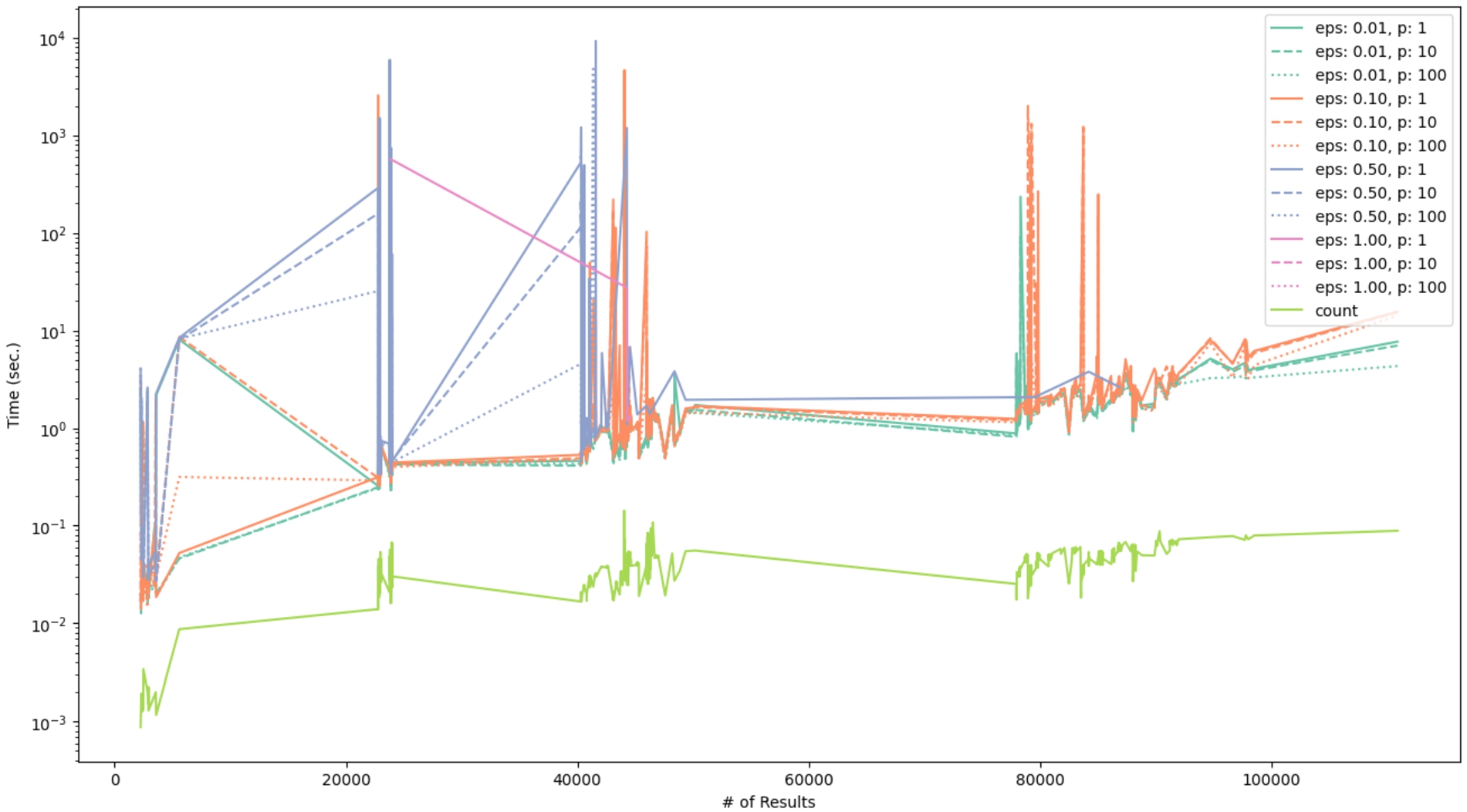
Fig. 20.
Execution time of the CLUSTER BY queries using k-medoids clustering.
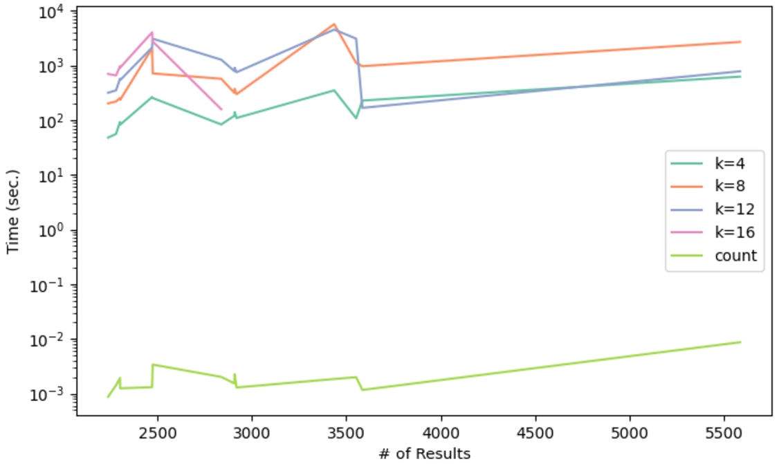
k-medoids is the costliest clustering algorithm of the three, as it minimises intra-cluster distance while maximising inter-cluster distance. Since the implementation requires to compute all pairwise distances first,
Given these experimental results, we can argue that the preferred way to cluster query results would be to use k-means, which shall have a similar execution time as the underlying query. Moreover, the k-medoids clustering algorithm should be avoided given its intensive memory and time usage. For the case of DBSCAN, it is necessary to be familiar with the vector space that is being generated, and carefully choose the parameters, for which we refer to the recommendations of Schubert et al. [39], of using
7.Concluding remarks
In this paper we have presented two extensions to SPARQL that incorporate two new similarity-based operators: similarity join and clustering. We define each operator’s syntax and semantics as part of the SPARQL grammar and the SPARQL algebra, and show how these new operators can be combined with the rest. In the case of the similarity join, we prove algebraic properties and rewriting equivalences. For the case of the clustering solution modifier, we discuss how it interacts with the other solution modifiers, such as GROUP BY. We motivate the importance of these extensions by defining use-case queries ranging several domains (images, stellar data, encyclopaedic data).
These operators have been implemented on top of Apache Jena, and the implementation is publicly available. We provide experimental results to evaluate the performance of the implementation, where we show that our similarity join outperforms the closest system to ours, DBSimJoin. We also offer comparisons among different methods and configurations to evaluate both the similarity join and the clustering. We determine that the better way to compute the similarity join is the vp-tree when there is a large number of solution mappings, and the nested loop when there are fewer solution mappings. For these experiments, we use 2,726 real SPARQL queries obtained from the logs of Wikidata. We also show that, when clustering, users may prefer to use the k-means algorithm, as it is faster and consumes less memory than k-medoids. We conclude by observing that DBSCAN is rather unpredictable in terms of execution time, and that it can produce useful and fast results if the parameters are carefully chosen.
As a future direction for this work, we plan to implement the physical operators using algorithms for secondary memory. This would allow for more efficient query processing and improved scalability, which has been an issue in particular for k-medoids clustering. Furthermore, we could design tailored algorithms that can take advantage of the database setting and the features of SPARQL, to further optimise the query processing.
Notes
1 We also directly standardise the units of measure. In practice, Wikidata allows for using a broad selection of different units, but the RDF export additionally provides reification properties that map these values to normalised values with the base S.I. unit of measure.
2 Using that
6 Retrieved from https://triplydb.com/RosalinedeHaan/iris. Credit to Rosaline de Haan.
7 The CSV data is available at http://burro.astr.cwru.edu/Academics/Astr221/HW/HW5/yaletrigplx.dat.
9 We use the dump from February 2020.
10 So long as X and Y always return some variable in common, then an antijoin
Acknowledgements
This work was partly funded by ANID – Millennium Science Initiative Program – Code ICN17_002, by the Swedish Research Council (Vetenskapsrådet, project reg. no. 2019-05655), and the CENIIT program at Linköping University (project no. 17.05). Hogan was supported by Fondecyt Grant 1221926
Appendices
Appendix
AppendixProofs of algebraic properties
This section presents proofs for the algebraic properties of the similarity join operator introduced in Section 4.2.
Example A.1.
To provide examples of the algebraic properties, and illustrate the ideas behind the proofs, we consider the following sets of solution mappings
Let
Proposition A.1.
Proof.
Assume
Example A.2.
Referring back to Example A.1, with respect to commutativity, note that:
Since the natural join operator is commutative, the distance measure symmetric, and the solution mappings unordered (recall that
With respect to left-distributivity, for example, note that:
Proposition A.2.
Proof.
As counter examples for commutativity and distributivity, note that there exist sets of mappings X, Y, Z with
– Commutativity:
– Distributivity:
Hence the result holds:
Example A.3.
Referring back to Example A.1,
Proposition A.3.
Proof.
Assume
Example A.4.
Referring back to Example A.1, we will look at the case of
Hence we can apply the union of the left-hand side of a k-nn similarity join first (per
Proposition A.4.
Proof.
As a counter example, consider that
Example A.5.
Taking
Proposition A.5.
Let
1.
2.
3.
 if
if 4.
Proof.
We prove each claim in the following:
1. The third step here is possible as ϕ does not rely on Z (per the assumptions).
2. For a mapping
3. The second step here uses the previous two results. The third step uses the right-distributivity of
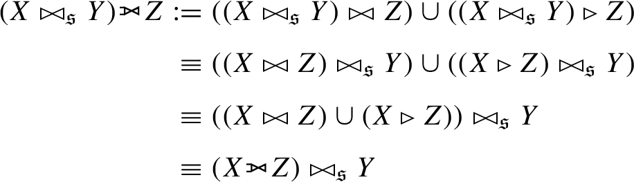
4. For a mapping
Example A.6.
We will look at examples for each claim:
1. Take
This equality would not hold if2. Recalling that ⊳ denotes an antijoin,1010 take the query
Aside from the conditions previously discussed for the first claim, such equalities apply for antijoins so long as the right operand of the antijoin (in this case
3. Recalling that
 denotes a left-join (or OPTIONAL in SPARQL), take the query
  , which gives:
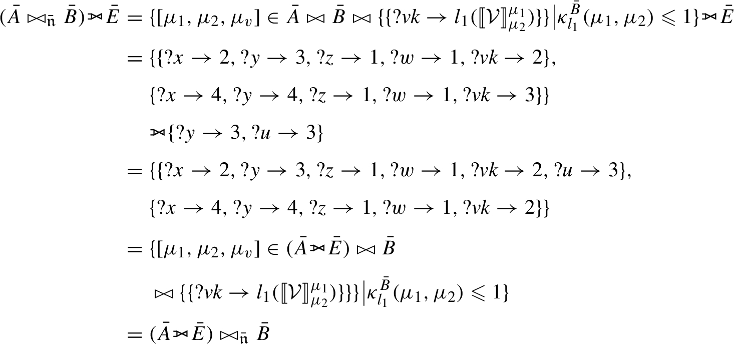
The same conditions as applied before in the second case apply again here.
4. Let
Added to the base conditions of claim 1, such equalities only hold so long as all the variables that
References
[1] | R. Battle and D. Kolas, Enabling the geospatial Semantic Web with Parliament and GeoSPARQL, Semantic Web 3: (4) ((2012) ), 355–370. doi:10.3233/SW-2012-0065. |
[2] | F. Belleau, M.-A. Nolin, N. Tourigny, P. Rigault and J. Morissette, Bio2RDF: Towards a mashup to build bioinformatics knowledge systems, Journal of Biomedical Informatics 41: (5) ((2008) ), 706–716, https://www.sciencedirect.com/science/article/pii/S1532046408000415. doi:10.1016/j.jbi.2008.03.004. |
[3] | C. Böhm, B. Braunmüller, F. Krebs and H.-P. Kriegel, Epsilon Grid Order: An Algorithm for the Similarity Join on Massive High-Dimensional Data, Association for Computing Machinery, New York, NY, USA, (2001) , pp. 379–388, ISSN 0163-5808. doi:10.1145/376284.375714. |
[4] | C. Böhm and F. Krebs, Supporting KDD applications by the k-nearest neighbor join, in: Database and Expert Systems Applications, V. Mařík, W. Retschitzegger and O. Štěpánková, eds, Springer Berlin Heidelberg, Berlin, Heidelberg, (2003) , pp. 504–516. ISBN 978-3-540-45227-0. doi:10.1007/978-3-540-45227-0_50. |
[5] | J.-P. Dittrich and B. Seeger, GESS: A scalable similarity-join algorithm for mining large data sets in high dimensional spaces, in: Proceedings of the Seventh ACM SIGKDD International Conference on Knowledge Discovery and Data Mining, KDD ’01, Association for Computing Machinery, New York, NY, USA, (2001) , pp. 47–56. ISBN 158113391X. doi:10.1145/502512.502524. |
[6] | V. Dohnal, C. Gennaro, P. Savino and P. Zezula, D-index: Distance searching index for metric data sets, Multimedia Tools and Applications 21: (1) ((2003) ), 9–33. doi:10.1023/A:1025026030880. |
[7] | M. Ester, H.-P. Kriegel, J. Sander, X. Xu et al., A density-based algorithm for discovering clusters in large spatial databases with noise, in: Proceedings of the 2nd ACM International Conference on Knowledge Discovery and Data Mining (KDD), Vol. 96: , (1996) , pp. 226–231. |
[8] | S. Ferrada, B. Bustos and A. Hogan, IMGpedia: A linked dataset with content-based analysis of Wikimedia images, in: The Semantic Web – ISWC 2017, Springer International Publishing, Cham, (2017) , pp. 84–93. ISBN 978-3-319-68204-4. doi:10.1007/978-3-319-68204-4_8. |
[9] | S. Ferrada, B. Bustos and A. Hogan, Extending SPARQL with similarity joins, in: The Semantic Web – ISWC 2020, Springer International Publishing, Cham, (2020) , pp. 201–217. ISBN 978-3-030-62419-4. doi:10.1007/978-3-030-62419-4_12. |
[10] | M. Galkin, M. Vidal and S. Auer, Towards a multi-way similarity join operator, in: New Trends in Databases and Information Systems, Springer International Publishing, Cham, (2017) , pp. 267–274. ISBN 978-3-319-67162-8. doi:10.1007/978-3-319-67162-8_26. |
[11] | G. Giacinto, A nearest-neighbor approach to relevance feedback in content based image retrieval, in: Proceedings of the 6th ACM International Conference on Image and Video Retrieval, CIVR ’07, Association for Computing Machinery, New York, NY, USA, (2007) , pp. 456–463. ISBN 9781595937339. doi:10.1145/1282280.1282347. |
[12] | R. Guerraoui, A.-M. Kermarrec, O. Ruas and F. Taïani, Fingerprinting big data: The case of KNN graph construction, in: 2019 IEEE 35th International Conference on Data Engineering (ICDE), (2019) , pp. 1738–1741. doi:10.1109/ICDE.2019.00186. |
[13] | S. Guha, R. Rastogi and K. Shim, CURE: An efficient clustering algorithm for large databases, SIGMOD Rec. 27: (2) ((1998) ), 73–84. doi:10.1145/276305.276312. |
[14] | A. Guttman, R-Trees: A Dynamic Index Structure for Spatial Searching, Vol. 14: , ACM, (1984) . |
[15] | S. Harris, A. Seaborne and E. Prud’hommeaux, SPARQL 1.1 Query Language, (2013) , https://www.w3.org/TR/sparql11-query/. |
[16] | A. Hogan, M. Mellotte, G. Powell and D. Stampouli, Towards fuzzy query-relaxation for RDF, in: The Semantic Web: Research and Applications, Springer Berlin Heidelberg, Berlin, Heidelberg, (2012) , pp. 687–702. doi:10.1007/978-3-642-30284-8_53. |
[17] | E.H. Jacox and H. Samet, Metric space similarity joins, ACM Trans. Database Syst. 33: (2) ((2008) ). doi:10.1145/1366102.1366104. |
[18] | G. Karypis, E.-H. Han and V. Kumar, Chameleon: Hierarchical clustering using dynamic modeling, Computer 32: (8) ((1999) ), 68–75. doi:10.1109/2.781637. |
[19] | L. Kaufman and P.J. Rousseeuw, Finding Groups in Data: An Introduction to Cluster Analysis, John Wiley & Sons, (2009) . |
[20] | C. Kiefer, A. Bernstein and M. Stocker, The fundamentals of iSPARQL: A virtual triple approach for similarity-based Semantic Web tasks, in: The Semantic Web, Springer Berlin Heidelberg, Berlin, Heidelber, (2007) , pp. 295–309. doi:10.1007/978-3-540-76298-0_22. |
[21] | A. Ławrynowicz, Query results clustering by extending SPARQL with CLUSTER BY, in: On the Move to Meaningful Internet Systems: OTM 2009 Workshops, Springer Berlin Heidelberg, Berlin, Heidelberg, (2009) , pp. 826–835. ISBN 978-3-642-05290-3. doi:10.1007/978-3-642-05290-3_101. |
[22] | C. Li, M. Wang, L. Lim, H. Wang and K.C.-C. Chang, Supporting ranking and clustering as generalized order-by and group-by, in: Proceedings of the 2007 ACM SIGMOD International Conference on Management of Data, SIGMOD ’07, Association for Computing Machinery, New York, NY, USA, (2007) , pp. 127–138. ISBN 9781595936868. doi:10.1145/1247480.1247496. |
[23] | H. Li, X. Zhang and S. Wang, Reduce pruning cost to accelerate multimedia kNN search over MBRs based index structures, in: 2011 Third International Conference on Multimedia Information Networking and Security, (2011) , pp. 55–59. doi:10.1109/MINES.2011.85. |
[24] | J. MacQueen et al., Some methods for classification and analysis of multivariate observations, in: Proceedings of the Fifth Berkeley Symposium on Mathematical Statistics and Probability, Vol. 1: , Oakland, CA, USA, (1967) , pp. 281–297. |
[25] | S. Mahran and K. Mahar, Using grid for accelerating density-based clustering, in: 2008 8th IEEE International Conference on Computer and Information Technology, (2008) , pp. 35–40. doi:10.1109/CIT.2008.4594646. |
[26] | M. Muja and D.G. Lowe, Fast approximate nearest neighbors with automatic algorithm configuration, in: International Joint Conference on Computer Vision, Imaging and Computer Graphics Theory and Applications (VISSAPP), INSTICC Press, (2009) , pp. 331–340. |
[27] | G. Navarro, Analyzing metric space indexes: What for? in: 2009 Second International Workshop on Similarity Search and Applications, (2009) , pp. 3–10. doi:10.1109/SISAP.2009.17. |
[28] | T. Neumann and G. Moerkotte, Characteristic sets: Accurate cardinality estimation for RDF queries with multiple joins, in: 2011 IEEE 27th International Conference on Data Engineering, (2011) , pp. 984–994. doi:10.1109/ICDE.2011.5767868. |
[29] | A.N. Ngomo and S. Auer, LIMES – a time-efficient approach for large-scale link discovery on the web of data, in: International Joint Conference on Artificial Intelligence (IJCAI), (2011) , pp. 2312–2317. |
[30] | R. Oldakowski and C. Bizer, SemMF: A framework for calculating semantic similarity of objects represented as RDF graphs, poster at ISWC. (2005) . |
[31] | B.C. Ooi, Spatial kd-tree: A data structure for geographic database, in: Datenbanksysteme in Büro, Technik und Wissenschaft, Springer, (1987) , pp. 247–258. doi:10.1007/978-3-642-72617-0_17. |
[32] | C. Ordonez and E. Omiecinski, Efficient disk-based k-means clustering for relational databases, IEEE Transactions on Knowledge and Data Engineering 16: (8) ((2004) ), 909–921. doi:10.1109/TKDE.2004.25. |
[33] | R. Paredes and N. Reyes, Solving similarity joins and range queries in metric spaces with the list of twin clusters, Journal of Discrete Algorithms 7: (1) ((2009) ), 18–35. doi:10.1016/j.jda.2008.09.012. |
[34] | J. Pérez, M. Arenas and C. Gutiérrez, Semantics and complexity of SPARQL, ACM TODS 34: (3) ((2009) ), 16:1–16:45. doi:10.1145/1567274.1567278. |
[35] | A. Petrova, E. Sherkhonov, B. Cuenca Grau and I. Horrocks, Entity comparison in RDF graphs, in: The Semantic Web – ISWC 2017, Springer International Publishing, Cham, (2017) , pp. 526–541. ISBN 978-3-319-68288-4. doi:10.1007/978-3-319-68288-4_31. |
[36] | E. Prud’hommeaux, SPARQL query language for RDF, (2008) , http://www.w3.org/TR/rdf-sparql-query/. |
[37] | L. Qi, H.T. Lin and V. Honavar, Clustering remote RDF data using SPARQL update queries, in: 2013 IEEE 29th International Conference on Data Engineering Workshops (ICDEW), (2013) , pp. 236–242. doi:10.1109/ICDEW.2013.6547456. |
[38] | E. Schubert and P.J. Rousseeuw, Fast and eager k-medoids clustering: |
[39] | E. Schubert, J. Sander, M. Ester, H.P. Kriegel and X. Xu, DBSCAN revisited, revisited: Why and how you should (still) use DBSCAN, ACM Trans. Database Syst. 42: (3) ((2017) ). doi:10.1145/3068335. |
[40] | M.A. Sherif and A.N. Ngomo, A systematic survey of point set distance measures for link discovery, Semantic Web 9: (5) ((2018) ), 589–604. doi:10.3233/SW-170285. |
[41] | K. Shim, R. Srikant and R. Agrawal, High-Dimensional Similarity Joins, (2002) , pp. 156–171. doi:10.1109/69.979979. |
[42] | Y.N. Silva, W.G. Aref and M.H. Ali, Similarity group-by, in: 2009 IEEE 25th International Conference on Data Engineering, (2009) , pp. 904–915. doi:10.1109/ICDE.2009.113. |
[43] | Y.N. Silva, S.S. Pearson and J.A. Cheney, Database similarity join for metric spaces, in: Similarity Search and Applications, Springer Berlin Heidelberg, Berlin, Heidelberg, (2013) , pp. 266–279. doi:10.1007/978-3-642-41062-8_27. |
[44] | J. Volz, C. Bizer, M. Gaedke and G. Kobilarov, Discovering and maintaining links on the web of data, in: The Semantic Web – ISWC 2009, Springer Berlin Heidelberg, Berlin, Heidelberg, (2009) , pp. 650–665. ISBN 978-3-642-04930-9. doi:10.1007/978-3-642-04930-9_41. |
[45] | D. Vrandečić and M. Krötzsch, Wikidata: A free collaborative knowledgebase, Communications of the ACM 57: ((2014) ), 78–85. doi:10.1145/2629489. |
[46] | W. Wang, J. Yang, R. Muntz et al., STING: A statistical information grid approach to spatial data mining, in: Very Large Data Bases Conference (VLDB), Vol. 97: , (1997) , pp. 186–195. |
[47] | X. Xu, M. Ester, H.-P. Kriegel and J. Sander, A distribution-based clustering algorithm for mining in large spatial databases, in: Proceedings 14th International Conference on Data Engineering, (1998) , pp. 324–331. doi:10.1109/ICDE.1998.655795. |
[48] | P.N. Yianilos, Data structures and algorithms for nearest neighbor search in general metric spaces, in: Symposium on Discrete Algorithms (SODA), Vol. 93: , (1993) , pp. 311–321. |
[49] | P. Zezula, G. Amato, V. Dohnal and M. Batko, Similarity Search: The Metric Space Approach, Vol. 32: , Springer Science & Business Media, (2006) . |
[50] | X. Zhai, L. Huang and Z. Xiao, Geo-spatial query based on extended SPARQL, in: 2010 18th International Conference on Geoinformatics, (2010) , pp. 1–4. doi:10.1109/GEOINFORMATICS.2010.5567605. |
[51] | C. Zhang and Y. Huang, Cluster by: A new SQL extension for spatial data aggregation, in: Proceedings of the 15th Annual ACM International Symposium on Advances in Geographic Information Systems, GIS ’07, Association for Computing Machinery, New York, NY, USA, (2007) . ISBN 9781595939142. doi:10.1145/1341012.1341077. |
[52] | T. Zhang, R. Ramakrishnan and M. Livny, BIRCH: An efficient data clustering method for very large databases, SIGMOD Rec. 25: (2) ((1996) ), 103–114. doi:10.1145/235968.233324. |
[53] | A. Zimek, E. Schubert and H.-P. Kriegel, A survey on unsupervised outlier detection in high-dimensional numerical data, Science Journal 5: (5) ((2012) ), 363–387. doi:10.1002/sam.11161. |

