INK: Knowledge graph representation for efficient and performant rule mining

Steenwinckel, Bram; De Turck, Filip; Ongenae, Femke

doi:10.3233/SW-233495

INK: Knowledge graph representation for efficient and performant rule mining

Article type: Research Article

Authors: Steenwinckel, Bram^{; *} | De Turck, Filip | Ongenae, Femke

Affiliations: Internet and Data Lab, Ghent University, Technologiepark-zwijnaarde 126, Gent, Belgium

Correspondence: [*] Corresponding author. E-mail: [email protected].

Keywords: Knowledge representation, semantic rule mining

DOI: 10.3233/SW-233495

Journal: Semantic Web, vol. Pre-press, no. Pre-press, pp. 1-22, 2023

Published: 2 October 2023

Get PDF

Abstract

Semantic rule mining can be used for both deriving task-agnostic or task-specific information within a Knowledge Graph (KG). Underlying logical inferences to summarise the KG or fully interpretable binary classifiers predicting future events are common results of such a rule mining process. The current methods to perform task-agnostic or task-specific semantic rule mining operate, however, a completely different KG representation, making them less suitable to perform both tasks or incorporate each other’s optimizations. This also results in the need to master multiple techniques for both exploring and mining rules within KGs, as well losing time and resources when converting one KG format into another. In this paper, we use INK, a KG representation based on neighbourhood nodes of interest to mine rules for improved decision support. By selecting one or two sets of nodes of interest, the rule miner created on top of the INK representation will either mine task-agnostic or task-specific rules. In both subfields, the INK miner is competitive to the currently state-of-the-art semantic rule miners on 14 different benchmark datasets within multiple domains.

1.Introduction

Knowledge graphs (KGs) are increasingly used as data structures to combine domain expertise with raw data values [11]. In this work, we refer to a KG as a multi-relational directed graph, G=(V,E), where V are the vertices or entities in our graph and E the edges or predicates. The example KG represented in Fig. 1 shows eight interlinked nodes describing four members of the band Coldplay. Three of these members have a common subgraph as they all studied and were born in England. One member was born in Scotland which is, at time of writing, still a part of the United Kingdom (UK).

Fig. 1.

Simple example of a KG, extracted from DBpedia [1]. Eight nodes are defined, linked to each other by four unique labelled edges.

Numerous applications are built upon these KGs, covering various domains such as industry 4.0, pervasive health and smart cities [2,27,30]. These applications interact with the KGs directly or transform the graph into a vector representation to perform Machine Learning (ML) related tasks [13]. Rule mining is also such a KG application, where the goal is to find logical rules in a given KG. For example, a rule mining application for the given example KG in Fig. 1 could find the logical rule: If X has Alma mater Y and Y is Located In Z, Then X is born in Z. Such logical rules will come with a certain confidence score, defining the general applicability of the rule. The more reliable rules can then be used to complete the KG, perform downstream tasks such as fact prediction, fact checking or anomaly and error detection.

Rule mining is part of data mining in general, where two broad subfields exist. On the one hand, there is task-agnostic or descriptive mining, where one wants to mine some general information about the KG or some general facts, which hold beyond this provided KG and are generally applicable. This subfield was originally created to discover hidden knowledge from transactional data, such as relational databases. Association Rule Mining (ARM) is the best-known descriptive technique. A transaction in ARM is an observation of the co-occurrence of a set of items. One possible way to apply ARM to semantic data or KGs is by converting the internal representation to a set of transactions. ARM thus identifies the transactions that identify co-occurrences of items that appear frequently in the KG by calculating the associated metrics to quantify this, such as the confidence and the support of the transactions. The logical rule defined, If X has Alma mater Y and Y is Located In Z, Then X is born in Z, is such a possible hidden rule that could be mined with an ARM application. ARM for KGs is used in data integration and KG completion tasks [4,22].

On the other hand, prescriptive mining is more task-specific and performs inferences on the current data, to make predictions in the future [12]. Inductive Logic Programming (ILP) is the best-known paradigm in this subfield. The ILP techniques deduce logical rules from a positive set of nodes and require some (generated) negative set of counter-examples. An example ILP task could be to find one general rule to describe all four members of the Coldplay band in Fig. 1. The positive set of nodes selected for this mining task are underlined in Fig. 1. One possible rule could state the born In ?x and ?x Part of UK relationships hold for all members.

Both subfields are complementary. While the ILP field is able to handle task-agnostic cases, it is most known by its task-specific capabilities, as specific facts are needed for those cases. Therefore, ILP directly captures the available related information in the KG to generate the rules. The ILP program will immediately use the available predicate-object information to discriminate between the provided positive and negative set. ILP can, however, be relatively slow and can therefore not handle the huge amount of data that KGs provide today. ARM can handle large KGs and generate rules for fully task-agnostic problems. It is fast and scales to large graphs. This often results in the fact that ARM generates a lot of nonsense or too generally applicable rules as it considers all triples or facts. The generated ARM rule for our example KG is such a rule with limited effect, because people do not always study where they were born.

There does not exist a technique which can perform both prescriptive (task-specific) and descriptive (task-agnostic) rule mining for KGs. The main reason, to our knowledge, is that the current techniques available for both tasks require a different internal representation of the KG. These transformations are performed in relation to the subfield they are operating on. ARM mainly requires the KG to be represented as transactions, which reduces the linked aspects of the existing KG. ILP directly works on the graph representation itself, leading to the earlier discussed performance issues.

The main contribution of this work is to use the existing paradigms of rule mining within ML such as ILP and ARM directly on the KG to perform both task-specific and task-agnostic rule mining tasks. We propose a technique to perform such rule mining on KGs by Instance Neighbouring using Knowledge (INK) [28]. INK represents a KG by analysing the neighbourhoods of selected nodes of interest. Given a set of nodes of interest T, a subset of V, INK finds all paths with a certain depth D starting from T. By marking each path with its destination, a binary feature set is created for each node within T that can be used in further downstream tasks. In the case of mining rules over the whole KG, T will be equal to V and a mining algorithm was developed to search for frequently occurring combinations of relationships within the INK representation. When a more specific task is given, only the neighbourhoods of the nodes which have to be considered are taken into account. An interpretable ML rule set approach was adapted to work with the INK representation to mine the relevant rules.

Combining these ILP and ARM techniques into a framework that is capable of directly mining the most interesting rules, without changing the internal representation of the KG, makes INK capable of seamlessly switching between task-agnostic and task-specific rule mining. This makes INK capable of dealing with varying scenarios and use cases without the need to change the internal representation.. For both these mining paradigms, INK is able to capture the complexity of the KG in an efficient manner.

The remainder of this paper is structured as follows. Section 2 gives an overview of the currently available semantic rule mining techniques for both the task-agnostic and task-specific field. Section 3 details the INK KG representation. Section 4 shows how INK can be incorporated into a rule mining system. Both the implementation of INK and the accompanying rule miner are discussed in Section 5. In Section 6, we evaluate INK for both the task-agnostic and task-specific rule mining, and compare the results with the current state-of-the-art. Section 7 discusses the advantages and drawbacks of INK in the perspective of task-agnostic and task-specific mining. At last, the conclusion of this work is provided in Section 8.

2.Related work

Rule mining has a long history, but the existing techniques can be either based on ARM or ILP. ARM searches for implication (if … then …) rules, such as “If a person X has an Alma mater Y, and Y is located in Z, then X is born in Z”. ILP techniques deduce logical rules from ground facts. Using ILP in the perspective of task-specific rule mining might use negative statements as counterexamples to optimize the mining process. For task-agnostic cases, this counterexample generation process is not necessarily required. In this section, the applicability of both these techniques for either task-specific, task-agnostic or both are described in the context of KGs.

2.1.Task-agnostic semantic rule mining

Task-agnostic semantic rule mining is the term that relates the closest to the general description of rule mining within ML. The goal of rule mining here is to find a rule or pattern for those examples that frequently occur together. The approach relies on the generation of so-called frequent itemsets, where sets of two or more items occurring together are combined with other itemsets to create rules [36]. Within the realm of KGs, task-agnostic rule mining approaches are less dependent upon the generation of these frequent itemsets. The goal is also different: the rule mining process tries to derive new facts and complete an existing KG, improve the reasoning quality or help to identify potential errors [14].

The rules generated within these KG rule miners are Horn clauses and are denoted as Horn rules when they contain an implication. They usually consist of a head and a body, where the head is a single atom:

B1∧B2∧⋯∧Bn⇒r(x,y)

with head r(x,y) and body B1∧B2∧⋯∧Bn. All these atoms in our head and body are binary predicates. The body atoms are, therefore, frequently represented as a binary vector B→. The rules state that if all instantiated body atoms appear in the KG, the head atom can be derived. Additional rule specifications can be introduced to reduce the search space. Searching for connected and closed rules that are not reflexive can be such a rule specification:

– A rule is connected if every atom is connected transitively to every other atom of the rule.
– A rule is closed if all its variables are closed. A variable is closed when it appears at least twice in the rule.
– A rule is reflexive if it contains atoms of the form r(x,x)

The example rule “If a person X has an Alma mater Y, and Y is located in Z, then X is born in Z” is an example of a connected and closed, not reflexive rule.

Solutions have been proposed for mining such rules in large KGs. These solutions, such as AMIE, use a generation-then-evaluation approach [20]. For example, given a head predicate (say born_in(x,y)), the available techniques first generate all possible rules within a certain length with this head predicate and then evaluate their quality to find high quality rules (such as alma_mater(x,y)∧located_in(y,z)→born_in(x,y)). To define whether a rule is of high quality, widely used statistical measurement, such as support and confidence, from the ML rule mining field were used.

The support of a rule quantifies the number of correct predictions in the existing KG. More in general, the support of a rule R in a KG G is the number of true derivations r(x,y) (with r(x,y) the head atom as explained above) that the rule makes in the KG:

support(R)=|{r(x,y):(G∧R⊧r(x,y))∧r(x,y)∈G}|

By providing a threshold on this support value, rules and facts which are less common can be pruned.

Confidence is a measure that also takes the incorrect rule implications into account. The standard confidence of a rule is the ratio of all its predictions that are in the KG. All facts that are not in the KG are seen as negative evidence.

conf(B→⇒r(x,y))=support(B→⇒r(x,y))|(x,y):B→|

Despite the fact that approaches like AMIE could mine rules from large KGs, the efficiency and effectiveness needed to be improved to overcome many drawbacks. ML rule mining operates under the closed world assumption: a statement that is true is also known to be true and conversely, what is not currently known to be true, is false and introduces negative evidence for those cases which are not available in the dataset. KGs can, however, be incomplete and follow the open world principle: the truth value of a statement may be true irrespective of whether or not it is known to be true [19]. The partial completeness assumption (PCA) is therefore proposed to debias the statistical estimation of the support and confidence measurements [7]. For efficiency, sampling and approximation measures [12] are adopted to reduce time overheads of accurate rule evaluations; besides, many efficiency optimizations are proposed [28] to speed up rule evaluation. All these modifications resulted in tools like AMIE+ and AMIE3 [16]. Nevertheless, the time-consuming candidate generation step is still inevitable.

The recent advances in the area of embeddings and KG vector representations resulted in some additional rule mining methods. The main goal of such miners is to deal with the possible incompleteness or large scale of the KGs, which reduces the need for partial completeness calculations [34]. One such miner is RuLes [10]. It iteratively constructs rules over a KG and collects feedback for assessing the quality of (partially constructed) rule candidates through specific queries issued to a precomputed embedding model. Within the Rules framework, the confidence measures capture the rule quality better than other techniques because they now reflect the patterns in the missing facts. The improved confidence measures, therefore, improve the ranking of rules. An embedded version of the KG is used here to define the quality of the rule and is not used to mine the task-agnostic rules themselves.

Another such technique is RLvLR (Rule Learning via Learning Representations) miner, an embedding-based approach to rule learning focusing on descriptive rule mining [21]. This miner specifies a target predicate in a KG to mine quality rules whose head has that predicate. The combination of the technique of embedding in representation learning together with a new sampling method results in more quality rules than major systems for rule learning in KGs such as AMIE+. The main focus of the RLvLR miner is defined in the scope of only mining specific rules for a given predicate. The RLvLR miner is, however, not made publicly available, except for an compiled executable to reproduce the fixed experimental setup.

2.2.Task-specific semantic rule mining

ILP was created in between the worlds of ML and Logic Programming where the logic programs or rules are derived from examples and the available KG. Rules here can be seen as hypotheses and the available examples are used to support the evidence for these hypotheses.

Learning hypotheses or descriptions for certain concepts gained interest in the field of ILP along the adoption of OWL and Description Logic (DL). Within this realm of concept learning, the obtained rules are different from the ones described in Section 2.1. Here, the logical rules capture the relationships and dependencies among attributes, providing explicit explanations of the learned concept based on the available data. The current state-of-the-art approaches for rule mining within ILP start from a general concept ⊤ (Thing) and further on refine this concept iteratively [5,18]. Learning algorithms can be designed by combining such a refinement operator with a search heuristic.

DL-Learner is such a tool that can learn logically entailed rules for a specific set of examples within a KG. The aim of DL-Learner is to find those rules covering as many positive examples while only applying to as few as possible negative examples [17]. Refinement operators are used to explore the search space of possible concept descriptions. Learning within DL-Learner can be seen as the search for such a correct rule description. Suitable operators to traverse the search space can be easily found but the goal of DL-Learner is to use those operators that have many useful properties like finiteness, non-redundancy, properness and completeness, while still allowing to efficiently traverse through the search space in pursuit of good hypotheses. DL-FOIL is another technique that uses refinement operators and progressively constructs the rule as a disjunction of partial descriptions [5]. Each partial description covers a part of the positive examples and rules out as many negative or uncertain membership examples as possible.

Both the strength of these two techniques is that they use reasoning techniques under the hood to derive expressive task-specific rules. On the other hand, this is also a weakness as it makes them less scalable and robust when they have to deal with large KGs. Large KGs might also result in a large search space when the conditions of the generated candidate rules never appear in the provided set of examples. Therefore, methods such as EvoLearner were designed that instead of refining the top concept ⊤, start with biassed random walks from the positive examples within the KG and use evolutionary algorithms to further refine these initial candidate rules [9].

Starting bottom-up (from the available positive and negative set) is quite common in the realm of ML. Here, the positive and negative sets are seen as data samples. The task is to find a good separation between these two sets. In addition to a reliable decision, one would also like to understand how this decision is generated, and more importantly, what the decision says about the data itself. Here, a few summarising and descriptive rules can provide intuition about the data and help to understand the decision process. The whole realm of interpretable ML models uses this idea to replace black-box models (e.g. random forests) with simpler models (e.g. rule sets) while improving interpretability and computational efficiency, without sacrificing predictive accuracy [24]. To our knowledge, none of these techniques are applied to KGs in a task-specific rule mining context, mainly due to the characteristics of the original graph representation.

2.3.Combining them both

The advancements within the ILP domain also resulted in task-agnostic techniques that use the available schema information within the knowledge graph to mine generic rules [8]. They can even be used for scheme completion or find faults within this schema level [3]. Those techniques are not optimised to solve task-specific problems, but can be applied for this when limiting, e.g., the search space to a specific predicate.

3.INK representation

While many task-specific and task-agnostic mining techniques use refinement operators to traverse the search space, INK builds its internal representation by transforming the neighbourhood of the nodes of interest into a binary matrix representation. With this binary matrix representation, column operations based and comparisons of columns for a large number of nodes of interest can be easily performed to reveal new patterns or rules. The binary representation can be seen as a KG embedding and was evaluated in this perspective for multiple node classification tasks [28]. To explain how this binary representation is built, we use the example KG visualised in Fig. 1 throughout this section.

3.1.Neighbourhood dictionary

INK operates by selecting nodes of interest. This can be both all nodes within a graph (for task-agnostic mining), as well as some nodes specified upfront (task-specific mining). In our example KG, we select two nodes of interest: Chris Martin and Guy Berryman. INK will first query the neighbourhood of a given depth for all these nodes of interest. If we define the depth parameter K to be two, the neighbourhood for Chris Martin will exist of the Alma mater and Born in relations, together with the neighbourhood of the University College London node providing the Located in relation and the neighbourhood of the England node with the Part of relation. To store these neighbourhoods efficiently, a dictionary representation is used. For a given node of interest, this dictionary is built in an iterative fashion. The predicates in a neighbourhood of depth one are inserted first into our dictionary, together with their corresponding objects as values. These dictionary values are lists, as a single predicate can occur multiple times with different objects in the neighbourhood of a node. For our given example node Chris Martin, we represent the neighbourhood at depth one by:

{ALMAMATER→[University College London],BORNIN→[England]}

To add the neighbourhoods of depths > one, INK concatenates the predicates together. By concatenating these relations, INK provides a path from the node of interest to another node within our graph without providing detailed information about all intermediate nodes on that path. However, this information is still available in the (key, value) pairs added to our dictionary at the lower neighbourhood’s depths. In our example node, the previous dictionary will be extended with the following (key, value) pairs at depth two:

ALMAMATER.LOCATEDIN→[England]BORNIN.PARTOF→[UK]

Here, we see a link from the node of interest to the UK node over the Born in relation. The Born in object value is not represented in this (key, value) pair, but was specified at the previous depth 1.

In several cases, it is also beneficial to indicate that the relationship itself within the neighbourhood of a node of interest is provided. The current dictionary structure does not explicitly indicate this presence. To ensure relationship edges within their neighbourhoods can be compared against each other on a predicate level, the transformation step will also explicitly state that a particular predicate is available:

ALMAMATER→True,BORNIN→True,ALMAMATER.LOCATEDIN→TrueBORNIN.PARTOF→True

Here, no lists were used as values for our dictionary as we just want to indicate a specific relationship is available for that particular node of interest.

Completely similar, the dictionary representation of Guy Berryman until depth 2 is:

{BORNIN→[Scotland],BORNIN.PARTOF→[UK]BORNIN→[True],BORNIN.PARTOF→[True]}

More in general, combined for all nodes of interest N, the initial data structure of INK uses the following list format:

[(n,neighbourhood(n,k))∀ n in N]

where the neighbourhood(n,k) is the function which outputs the dictionary representation for our node n till a defined depth k.

3.2.Binary format

As the [(n,neighbourhood(n,k))] representation is 3 dimensional (one axis for the nodes of interest, one for the dictionary relation keys and one for dictionary object list values), an additional transformation is required to provide a binary representation of this data. All of the object’s values inside our neighbourhood dictionary are combined using a delimiter § to their corresponding key. In the strict sense, the binary format is created by unravelling the lists within our dictionary by string concatenating them with the corresponding dictionary key. When our 3 dimension representation contains the following entry,

[(Guy Berryman,{BORNIN→[Scotland],BORNIN.PARTOF→[UK]BORNIN→[True],BORNIN.PARTOF→[True]})]

our string concatenation operation would create the following features for the Guy Berryman entry:

BORNIN§ScotlandBORNIN.PARTOF§UKBORNIN§TrueBORNIN.PARTOF§True

Such features can be easily represented in a binary matrix, indicating for e.g. Guy Berryman that those features hold using a Boolean mark. Creating this binary representation for only one node of interest is not that interesting. When we combine the created features till depth 2 for both Chris Martin and Guy Berryman, more features will be available and some of these features will be a discriminator for either one of them.

(1)ALMAMATER§University College London(2)BORNIN§England(3)BORNIN§Scotland(4)ALMAMATER.LOCATEDIN§England(5)BORNIN.PARTOF§UK(6)ALMAMATER§True(7)BORNIN§True(8)ALMAMATER.LOCATEDIN§True(9)BORNIN.PARTOF§True

The binary INK representation for both Chris Martin and Guy Berryman is visualised in Table 1. The rows are defined by the nodes of interest, such that each cell indicates whether or not the subject of interest contains the relation(s)§object value. In this matrix, column (3) is a specific feature (Born in§Scotland) for Guy Berryman and could be of interest to differentiate Guy Berryman from the other team members.

Table 1

INK’s binary representation of Chris Martin and Guy Berryman nodes in the example graph of Fig. 1

	(1)	(2)	(3)	(4)	(5)	(6)	(7)	(8)	(9)
Chris Martin	1	1	0	1	1	1	1	1	1
Guy Berryman	0	0	1	0	1	0	1	0	1

3.3.Extension modules

While the binary representation of INK reflects the whole KG, it can derive additional information based, e.g. datatype properties or the amount of relationships that are available. This subsection describes two optional extension modules which are available in INK.

3.3.1.Numerical inequality

To deal with numerical data, a preprocessing module will check if the values corresponding to a specific relation are all floats or integers for all the corresponding objects and nodes of interest. When such a relation is found, we build a set of all possible inequalities using all the found objects for that relation. In our example KG, we could add the birth year of all our Coldplay members, which would be an integer value. When this extension module is enabled, all these integer values will be stored inside a set. INK compares for each node of interest the value of the birth year relation with all possible values in our set and adds a new entry to our neighbourhood dictionary as follow:

BIRTHYEAR<l→[True or False]&l>=BIRTHYEAR→[True or False],∀l in inequality set

Concrete, eight new entries for will be added, describing if the birth year of Band Member X is smaller than the birth year of the Band Member Y, or if birth year of Band Member X is greater than or equal the birth year of the Band Member Y, with both X and Y ∈ Chis Martin, Will Champion, Guy Berryman, Jonny Buckland.

3.3.2.Relation count

Another preprocessing module is available in INK to deal with relations having more than one object value. It can be beneficial to indicate how many of these relationships are available for a given node of interest. Therefore, a module was added that counts the objects related to a relationship starting from the node of interest. This model adds new entries to the neighbourhoods dictionary indicating how many times the objects share the same relationship, starting from the node of interest. More specifically, if in our example graph Chris Martin would have a second alma mater relation, this module would add the following entry:

COUNT.ALMAMATER→[2]

This entry can be directly transformed to

COUNT.ALMAMATER§2

as described above. The previous inequality module can also use these counting values, as they are stored as integer values.

4.INK rule mining

The 2D matrix representation discussed above can be seen as a KG embedding and it was already evaluated regarding a node classification task in this perspective [28]. It can be used to perform both task-specific and task-agnostic rule mining. More in general, rules will be built based on the column description or features of our binary matrix, as shown in Table 1. The fourth column in this example, i.e. ALMAMATER.LOCATEDIN§England, already introduced implicitly a variable to ignore the specific alma mater located in England. This fourth column states that there is a relation from our nodes of interest about a non-specified university, school, or college that one formerly attended which is located in England. This column can be interpreted more formally by:

ALMAMATER(?i,?x)∧LOCATEDIN(?x, England)

with ?x and ?i a variable.

As both task-specific and task-agnostic techniques use this representation, the only difference between them is how they interact and extract the relevant information. The task-agnostic miner operates on the columns themselves, comparing the Boolean values to build so-called frequent itemsets and create the rules. The task-specific miner operates on the rows to differentiate between the nodes of interest. The task-specific miner uses the columns as features within its model to define a more specific rule given the task it wants to solve.

4.1.INK task-agnostic mining

To apply ML ARM techniques, the INK task-agnostic mining component must define frequent itemsets. Here, the frequent itemsets will be based on the columns of INK’s binary representation. But in order to build these frequent itemsets, we first have to extract the neighbourhood for all subject nodes containing a fact in our KG. For our example graph in Fig. 1, this means that not only the neighbourhoods for Chris Martin and Guy Berryman will be extracted, but also for all other nodes in our KG as they are also subjects of facts.

The frequent itemsets exist out of one or a combination of relationships accompanied with the calculated support. Despite the fact that many different combinations of relationships exist, INK use the anti-monotone property of support (adding a new relationship to a frequent itemset will never increase the support value) and searches for the following defined patterns in the KG:

(10)x→relationshipy

(12)x→relationship 1z→relationship 2y(13)x→relationship 1z←relationship 2y(14)x←relationship 1z→relationship 2y

The combination of some of these patterns could lead to a plausible rule within our KG. If we combine the patterns of (10) and (12) for example, the rule miner could create rules such as:

x→relationship 1z∧z→relationship 2y⟹x→relationship 3y

Traditional ML ARM rule mining techniques can easily derive these rules when the frequent itemset is being provided. The above derived rule was originated from the following frequent itemsets:

itemset1={x→relationship 1y}itemset2={x→relationship 2y}itemset3={x→relationship 3y}itemset4={x→relationship 1z,z→relationship 2y}itemset5={(x→relationship 1z,z→relationship 2y),x→relationship 3y}

Accompanying this itemset are all unique x & y nodes that hold for that itemset. The length of these unique node sets is our support metric.

INK actively searches for these itemsets within its 2D matrix representation. Some of these itemsets are trivial to calculate. The itemsets originating from pattern (10) described above can be easily identified within our matrix representation. INK extracts by default the relation§object columns but the task-agnostic miner is more interested in colums obeying the §object values. These columns already introduce a variable near the end, for example we can write alma mater(?x) to indicate that those columns contain an, not specified, alma mater, indicated through the variable x. Based on these relation columns, INK calculates the occurrence of the associated subject and object pairs. If the amount of pairs is higher than a defined support threshold, a frequent itemset for that specific relationship is created.

Frequent itemsets defined by the patterns in (11) and (12) might be harder to calculate. In traditional frequent itemset miners, the number of items inside the set must be defined upfront. Due to the INK relationship concatenation, they can be treated as the ones in (10). INK can fix the number of items within an itemset to two, as the depth parameter of the neighbourhood already implicitly introduces additional preconfigured items in our itemsets with possible lengths greater than one. In our example graph, the relation Alma mater.Located in is already such a predefined item, combining the Alma mater and Located in relationship. As this combined relation can already be found in the neighbourhood of the nodes of interest, there is a high chance that they can occur frequently together. When we add to this combined relation, a second, single relation, we implicitly have a frequent itemset of length 3 as shown above in itemset5. For example, if we combine Alma mater.Located in, with Born in, we get an itemset stating (ALMAMATER(?x,?y)∧LOCATEDIN(?y,?z),BORNIN(?x,?z)). However, purely algorithmic, the length of the itemset remains to two. We just provided additional variables within the items themselves to chain relationships, occurring frequently together, within the KG.

Computationally hard to calculate are the frequent itemsets belonging to patterns (13) and (14). Here the pairs of x & y have to be determined between two relationships where they share one variable z. These calculations are hard to perform efficiently in terms of time and memory ass,multiple intersections of x & y pairs have to be filtered to reduce the possible duplicate pairs. The INK miner will first find all z values in its 2D representation that are shared between two relationships as indicated in (13) and (14). Next, for each z, all x & y combinations are stored in a set. In the end, the length of this set is our support measure for this itemset.

Whether the items within an itemsets can be used in an interesting rule, depends on the calculated support value and corresponding threshold. The support for each itemset within INK is calculated using the following rule:

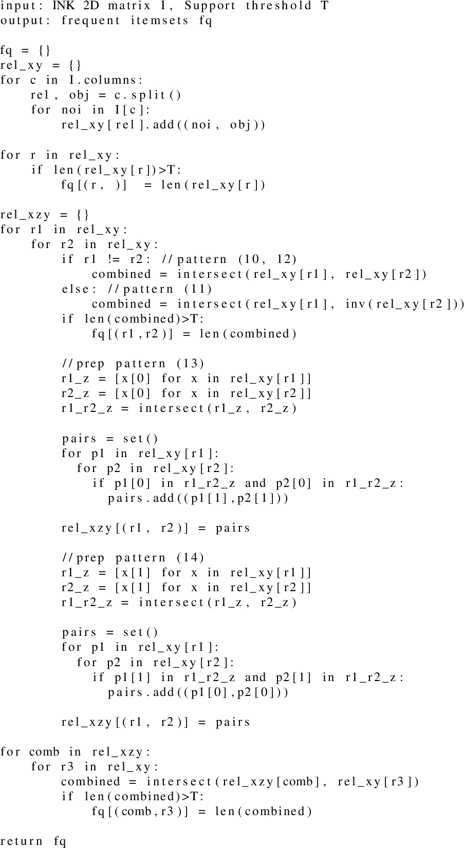
|∀R1 in Cink,∀R2 in Cink∑∀ o in OR1∩R2R1!=R2R1§o&R2§o|

Where Cink are all the relation-only columns of our INK representation, OR1∩R2 contains the intersection of all object values of the two relations R1 and R2 and & is the bitwise and operator. Note that both R1 and R2 can be a chain of relationships as discussed above and that the sets used to calculate the intersection are calculated upfront. The algorithm to define these itemsets for each of the provided patterns (10-14) is given in pseudocode in Listing 1.

Listing 1.

INK task-agnostic mining pseudocode

Based on these itemsets, we can select both an antecedent and consequent to get rules of interest. Measures such as confidence, lift and conviction are calculated from the support values and can be used to filter these rules.

INK is in this perspective also not limited to mine closed rules as any item within our itemset can be either head or body within our rule mining approach. The rule can still be connected. The head atom can also contain additional free variables due INK’s item representation within the frequent itemsets.

4.2.INK task-specific mining

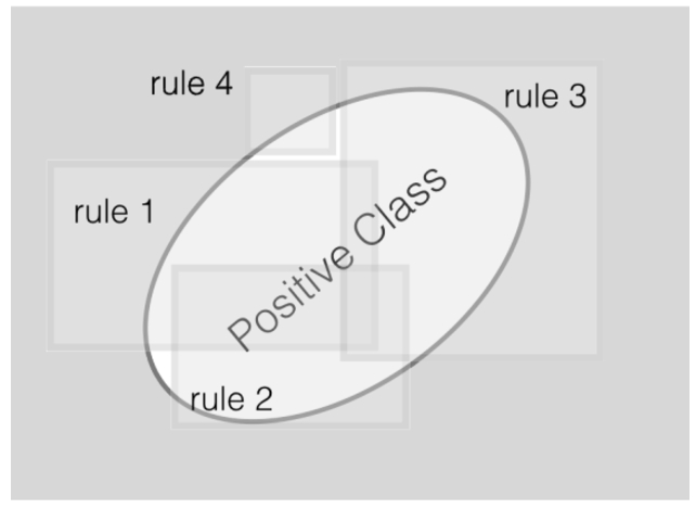
The INK 2D representation is used directly within a task-specific mining approach. The task-specific mining approach is based on the Bayesian rule set mining technique described by Wang et al. [32]. In this approach, the model consists of a set of rules and each rule is a conjunction of conditions. The model predicts that an observation is in a positive class when at least one of these rules is satisfied. In contrast, the observation belongs to the negative class if none of the rules apply. This problem is also visually represented in Fig. 2 where the goal is to find a set of rules for the positive class.

Fig. 2.

Illustration of a rule set. The area covered by any of the rule squares is classified as positive. Areas not covered by any rules are classified as negative. The goal is to select those rule areas within the positive class but with as minimal areas outside this oval.

More formally, a set of rules is denoted as R. Checking if one of the rules within R applies for a x within a dataset {xn,yn}n=1..N where yn∈0,1 and x∈V (as it is in our case a node of interest) can be performed by the general R(.) function. Let r represent a rule and r(.) a corresponding Boolean function:

r(.):V→{0,1}.

r(x) thereby identifies if x satisfies the rule r. Checking if this applies for the whole rule set can simply defined by:

R(x)=1∃r∈R,r(x)=1.0otherwise.

The approach described by Wang et al. optimises the search for these rule sets by relying on Bayesian analysis. In a first phase, candidate rules are generated using a random forest approach. Instead of using the created classifier, the rules within the built decision trees are collected and provided in a set. In a second phase, the rules are divided in different pools based upon their length. The length of a rule is defined upfront by the user. If the user sets the maximum rule length to L, L pools will be created. In the third phase, a globally optimised rule set is learned by considering both the accuracy and the interpretability of a model, while keeping computation simple. By controlling the parameters of the Bayesian prior, rules are drawn and combined independently from the pools. Large models are penalised. For the Bayesian Rule Set model, this results in a smaller number of rules. Since a small number of rules must cover the positive class, each rule in this model must cover as many observations as possible. To enforce this, a threshold on the number of examples satisfying the rule, more commonly known as the support of a rule, is introduced. It is due to this threshold that a significant reduction of the rule set’s search space can be made. Due to the anti-monotone property of the support metric, rules for which the support is initially too low will not be added to their corresponding Pool.

The required input for this Bayesian rule set mining is a binary matrix, which fits with the proposed INK representation of Section 3. This also means that this approach can’t work with numerical values such as floating points. INK is accompanied with several extension modules to enrich this binary representation, such that it can resolve these issues.

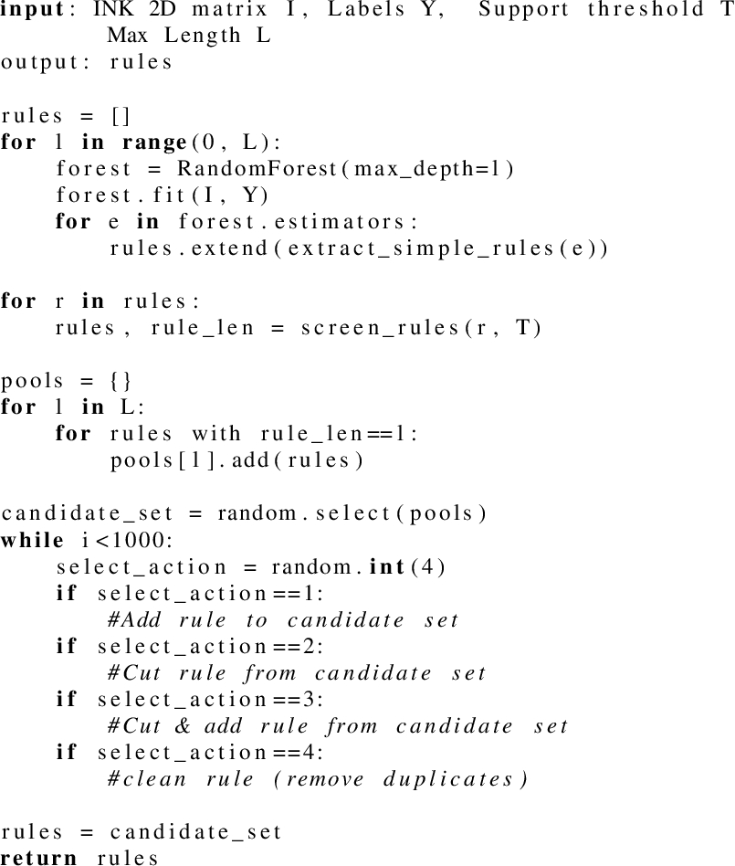
To train this model, INK will extract the neighbourhoods from two sets of nodes of interest, for a given depth parameter. One set contains all the positive nodes, the other set contains all negative ones. For task-specific cases, it is therefore required to specify these sets upfront. The labels for each node are stored in a different array. Optional parameters, such as the support, maximum length of the concatenation and the maximum number of rules in the rule set can be provided as input for the algorithm. A more formal algorithm is provided in pseudocode within Listing 2. Here we show the different aspects of rule set candidate generation and how 4 different actions influence the different rule candidate set. More information about the full implementation of this Bayesian Rule Set approach can be found in the original paper of Wang et al.

Listing 2.

INK task-agnostic mining pseudocode

The output of the Bayesian rule set mining module contains both the rules learned on the given training dataset to discriminate both positive and negative nodes of interest, as well the mechanism to evaluate the rules on the new unseen nodes.

5.Implementation

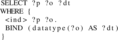
The INK representation described in Section 3 and the INK rule mining module of Section 4 are both implemented in Python. To extract the neighbourhoods for a given set of nodes of interest, a component was implemented which can query these relations iteratively. Two options are currently available inside this component: either a KG or a SPARQL endpoint is given as input. When a KG file is given, RDFLib [15] will be used to load the graph in the internal memory of the operating system. However, some large KGs can be hard to fit within the internal memory. Therefore, INK can use RDFLib in combination with the Header, Dictionary Triples (HDT) file format [6]. HDT compresses big RDF datasets while maintaining basic search operations, such as providing the neighbourhood of a node of interest. Listing 3 shows the query used for both options to extract the neighbourhood nodes and relation. The variable subject <ind> starts with the nodes of interest, but differs in each iteration given the graph. The datatype of the object within this query is used to determine if queried objects can be used as subjects in the next iteration (when the neighbourhood depth is not reached yet). The predicates and objects in each iteration are stored as described in Section 3. Python’s internal multiprocessing library is used to speed up the extraction of the neighbourhoods, as this operation can be performed over multiple processors given the amount of nodes of interest.

To transform the initial representation into a binary matrix, we used the Scikit-learn DictVectorizer [23] with the sparse option set to true and specifying the data type to be Boolean. This is necessary when we want to deal with large KGs and a large number of nodes of interest.

If positive and negative labels are defined together with these nodes of interest, the INK miner assumes a task-specific mining operation must be executed. Code from Wang et al. [32] was adapted to operate on our representation.

When no target array, task-agnostic mining is executed on the neighbourhoods of all nodes of interest. The task-agnostic code uses the MLxtend library [25] to produce the rules based on the calculated frequent itemsets, based on the INK representation.

The whole INK package is made available on GitHub.1 1

Listing 3.

SPARQL query

6.Evaluation set-up & results

Both the task-specific and task-agnostic mining capabilities are evaluated on multiple benchmark datasets as specified below. To extract the neighbourhoods of interest, all benchmark datasets were transformed to an HDT format such that the SPARQL query of listing 3 can be executed performant. All evaluations were performed on an Intel(R) Xeon(R) CPU E5-2650 v2 @ 2.60 GHz processor with 32 cores and 128 GB RAM.

Table 2

Comparison between INK and AMIE3 on 5 benchmark datasets. Both the average standard confidence measures and standard deviation (between brackets) for the best 10, 25 and top N rules of either INK or AMIE3 are visualised. N is determined by the minimum number of rules of either AMIE3 or INK. An indication of the total number of mined rules and the time it takes to run both INK and AMIE are provided

	Confidence Top 10		Confidence Top 25		Confidence Top N		# Rules		Duration (min)

	INK	AMIE3	INK	AMIE3	INK	AMIE3	INK	AMIE3	INK	AMIE3
Yago2	0.553 (0.09)	0.507 (0.08)	0.421 (0.13)	0.353 (0.15)	0.12 (0.15)	0.086 (0.13)	294	166	4.30	0.50
Yago2s	0.927 (0.05)	0.898 (0.08)	0.787 (0.14)	0.707 (0.18)	0.31 (0.24)	0.221 (0.23)	754	405	52.65	241.0
DBpedia 2.0	1.0 (0.0)	1.0 (0.0)	1.0 (0.0)	1.0 (0.0)	0.329 (0.27)	0.238 (0.3)	16957	8963	676.5	235.0
DBpedia 3.8	1.0 (0.0)	1.0 (0.0)	1.0 (0.0)	1.0 (0.0)	0.162 (0.22)	0.126 (0.21)	16499	9383	644.4	85.0
Wikidata	1.0 (0.0)	1.0 (0.0)	0.998 (0.0)	0.998 (0.0)	0.287 (0.29)	0.223 (0.3)	3993	2121	482.9	233.0

6.1.Task-agnostic evaluation

To compare the task independent rule mining capacities, we made a comparison between INK and AMIE3 on five benchmark datasets, which were already frequently used during various AMIE evaluations. Many competitors of AMIE exist as defined [35] and most of them improve the efficiency of the rule mining process, providing metrics to deal with the incompleteness of the KG and taking into account the open world assumption. This comparison focuses more on the quantitative mining capabilities of AMIE. YAGO (2 and 2s) is a semantic knowledge base derived from Wikipedia, WordNet and GeoNames [26]. The latest version, YAGO2s, contains 4.1M facts, where the first YAGO version contained 0.9M facts. The DBpedia datasets (2.0 and 3.8) are a subset of the crowd-sourced community effort to extract structured information from Wikipedia [1]. DBpedia 2.0 and DBpedia 3.8 contain 6.7M and 11.02M facts respectively. The Wikidata dataset is a Wikidata dump from December 2014 and contains 8.4M facts. Wikidata is a free, community-based knowledge base maintained by the Wikimedia Foundation with the goal to provide the same information as Wikipedia but in a computer-readable format [31]. All 5 benchmark datasets are made available by the Max Planck Institute.2 2

Both AMIE and INK prune rules based on both the default support level of 100 and a default max rule length of 3. To mine rules of length 3, the INK neighbourhood’s depth parameter was set to 2. This could result in rules containing atoms for both the head and body of length 2. When the support level of those atoms is above the provided thresholds, they can both be combined into a rule which implicitly results in a rule with length of 4. To make a fair quantitative comparison towards the mined AMIE rules of length 3, we filtered all those length 4 rules.

For all datasets, the average standard confidence of the top 10, top 25 and top N, with N the smallest number of rules from either INK or AMIE are compared as shown in Table 2. The standard deviation is provided between brackets. When, e.g., AMIE mines 166 rules and INK mines 294 rules, the Top N confidence will be the average of the 166 rules with the highest confidence for both AMIE and INK. The total number of filtered rules and the time it requires to mine these rules are also listed for both AMIE and INK.

6.2.Task-agnostic discussion

Compared to AMIE3, INK mined in all datasets more rules and most of these rules have also a high standard confidence level. The larger number of rules are mainly due to the fact that INK is also capable of analysing head atoms with more than 2 variables. While in previous works the perception raised that those rules could be neglected as their confidence level should be extremely low, INK showed that some of these rules do occur quite frequently in large datasets. An example of such a rule in DBpedia 3.8: ?a isCitizenOf ?b ⇒ ?a wasBornIn ?x ∧ ?x isLocatedIn ?b (confidence: 0.27). In this case, the introduction of the variable ?x in the head of the rule allows for more flexibility in capturing relationships between the entities involved. The rule suggests that if ?a is a citizen of ?b, then there exists some place ?x where ?a was born, and that place ?x is located in ?b. By allowing the introduction of new variables in the head, open rules can capture a wider range of associations and potentially discover more patterns in the data. Besides more flexibility, these non-closed rules enable the discovery of implicit relationships, such as the relationship between wasBornIn and isLocatedIn. As INK is not constrained to closed rules, it can extract more general rules that capture broader associations in the data. The downside is that these non-closed rules introduce additional complexity and require additional, mostly human-based, validation and interpretation. Post-processing analyses showed that all rules that were mined with AMIE were also available in the rules generated by INK. All additional INK rules were these non-closed or open rules, as the head atoms contain a variable inside the rule that didn’t occur in its body (such as the ?x in the example above). These rules can be of interest to either further summarise or investigate certain parts of our KG.

INK does have some disadvantages compared to AMIE3. INK consumes a large amount of RAM in order to build the internal representation and to generate the frequent itemsets. The time needed to create those rules is, except for the Yago2s dataset, substantially higher compared to INK. Further analyses, represented in Table 3, shows that the initial INK representation can be built quite fast and INK requires more time to actually mine all the relevant rules.

Table 3

Detailed overview of the embedding size and the time needed to create the INK representation for the task-agnostic rule mining datasets

	INK creation time (min)	#noi	#columns
Yago2	0.78	470483	607102
Yago2s	12.83	1653880	1057539
DBpedia 2.0	6.71	1376877	6946046
DBpedia 3.8	11.38	2198871	5647489
Wikidata	12.93	2990435	2983585

Another advantage of AMIE3 is that it is designed to mine rules iteratively and therefore uses less RAM to obtain rules. INK’s configuration settings are currently also limited as AMIE can also take into account constants, PCA confidence, removals of perfect rules, etc. INK does however have the capability to mine long rules (rules with a large amount of atoms) without expanding the frequent itemsets.

6.3.Task-specific evaluation

To compare the INK miner in the context of task-specific mining, we used the Structured Machine Learning benchmark framework (SML-Bench) [33]. This framework enables some specific tasks where structured hypotheses are learned from data with a rich internal structure or knowledge representation, usually in the form of one or more relations. The systems within this framework might differ in the knowledge representation languages they support and the programming languages they are written in. Many different systems can be incorporated within this SML-Bench framework but due to the nature of this paper regarding rule mining within KG, we selected those techniques from the related work in Section 2 that can be applied on KGs (more specifically, those techniques that take an OWL or triple file as input). INK was incorporated in this framework and a comparison was made between the top-down approach DL-learner and a bottom-up evolutionary approach EvoLearner. The code to incorporate INK within the SML-Bench framework is provided online3 3 such that INK can also be used in future evaluations.

Table 4

Overview of the datasets that are part of SML-Bench with their number of axioms (#A), classes (#C), object properties (#O), datatype properties (#D) and their description

Dataset	#A	#C	#O	#D	N.o.i.	pos/neg	Prediction of
Carcino	74,566	142	4	15	298	1.19	Carcinogenic drugs
Hepatitis	73,114	14	5	12	500	0.70	Hepatitis type based on patient data
Lympho	2,187	53	0	0	148	1.21	Diagnosis class based on lymphography patient data
Mammo	6,808	19	3	2	961	0.86	Breast cancer severity
Muta	62,066	86	5	6	42	0.44	Mutagenicity of chemical compounds
NCTRER	92,861	37	9	50	224	1.41	Molecule’s oestrogen receptor binding activity
Prem. League	214,566	10	14	202	81	0.97	Goal keepers based on player statistics
Pyrimidine	2,006	1	0	27	40	1.0	Inhibition activity of pyrimidines and the DHFR enzyme
Suramin	13,506	46	3	1	17	0.70	Suramin analogues for cancer treatment

In total, nine different datasets are available in the SML-Bench 3.0 version, all containing an OWL knowledge base and a single task based on two sets of files indicating the positive and negative nodes of interest. An overview of all these different datasets is provided in Table 4. All these datasets vary in terms of number of axioms, number of available classes, number of object and data properties. They all have a different amount of nodes of interest and can be either more or less balanced towards one class (either positive or negative).

The default SML-Bench configuration options were used within all our evaluations: 10-fold cross validation was used with a maximum execution time of 15 minutes for each fold. DL-learner version 1.5 was used with the SML-Bench default parameters for each learning task: For all tests, the CELEO algorithm was used to traverse the search space guided by the Pellet reasoner. By using these settings, DL-Learner will keep searching for relevant rules until the time threshold has passed. The optimised parameters provided by the original authors of the EvoLearner algorithm were used to evaluate their system. INK was initialised with a maximum neighbourhood depth of 3 such that the neighbourhoods of the neighbours from our start nodes were taken into account during the rule generation phase. The numerical levels and relation count extension modules described in Section 3.3 were also enabled. The OWL datasets were transformed into the HDT format, which was used as input to generate the INK representation. Four different metrics are reported in Table 5:

– Accuracy score: The number of correct predictions divided by all predictions. All learning tasks are binary classification problems, but can be unbalanced. We report the average accuracy score between 0 and 1 together with the standard deviation across the 10 folds.
– F1 score: The harmonic mean of the precision and recall: F1=2∗precision∗recallprecision+recall. Again, the average and standard deviation over 10 folds are reported.
– Matthews Correlation Coefficient (MCC): This metric takes into account the true and false positives and negatives and is generally regarded as a balanced measure which can be used even if the classes are of very different sizes: MCC=TP∗TN−FP∗FN(TP+FP)(TP+FN)(TN+FP)(TN+FN). MCC returns a value between −1 and +1: A coefficient of +1 represents a perfect prediction, 0 no better than random prediction and −1 indicates total disagreement between prediction and observation. Again, averages and standard deviations over 10 folds are reported.
– Duration: The time needed to find the most descriptive rule, based on the nine out of 10-folds + the time to evaluate this rule on one holdout fold. Averages and standard deviations over 10 folds are reported in seconds.

The results for each learning task are provided in Table 5. The task-specific rule mining results showed that INK is highly competitive with DL-Learner and is competitive in terms of time and predictive performance compared to EvoLearner.

Table 5

SML-Benchmark comparison between INK, DL-Learner (abbreviated by DL) and EvoLearner (abbreviated by Evo) for 4 metrics on 9 benchmark datasets. The results show both the average and standard deviation (between brackets) for a 10-fold cross validation evaluation

	Accuracy (std)			F1 (std)			MCC (std)			Duration (std)

	INK	DL	Evo	INK	DL	Evo	INK	DL	Evo	INK	DL	Evo
Carcino	0.56 (0.12)	0.54 (0.02)	0.66 (0.17)	0.47 (0.13)	0.70 (0.01)	0.72 (0.12)	0.18 (0.28)	0.00 (0.09)	0.31 (0.38)	191.4 (23.31)	888.3 (0.46)	146.7 (33.08)
Hepatitis	0.78 (0.03)	0.49 (0.06)	0.85 (0.04)	0.73 (0.07)	0.61 (0.03)	0.83 (0.05)	0.56 (0.09)	0.21 (0.07)	0.72 (0.06)	55.4 (1.28)	879.0 (0.0)	86.7 (12.61)
Lympho	0.80 (0.09)	0.82 (0.1)	0.80 (0.13)	0.82 (0.07)	0.86 (0.07)	0.84 (0.1)	0.64 (0.15)	0.67 (0.18)	0.62 (0.26)	33.3 (1.27)	873.7 (0.46)	45.7 (10.88)
Mammo	0.83 (0.04)	0.49 (0.02)	0.83 (0.04)	0.80 (0.05)	0.64 (0.01)	0.82 (0.05)	0.66 (0.07)	0.12 (0.1)	0.67 (0.08)	85.8 (2.52)	874.1 (0.3)	67.4 (3.04)
mutagenesis	0.98 (0.06)	0.94 (0.13)	1.0 (0.0)	0.97 (0.1)	0.93 (0.13)	1.0 (0.0)	0.96 (0.12)	0.9 (0.2)	1.0 (0.0)	31.4 (0.8)	883.0 (0.0)	53.6 (0.66)
NCTRER	0.99 (0.2)	0.59 (0.04)	1.0 (0.0)	0.99 (0.02)	0.73 (0.02)	1.0 (0.0)	0.98 (0.04)	0.01 (0.12)	1.0 (0.0)	201.9 (3.14)	885.2 (0.87)	242.0 (0.45)
Prem. League	0.99 (0.04)	DNF	1.0 (0.0)	0.99 (0.04)	DNF	1.0 (0.0)	0.98 (0.07)	DNF	1.0 (0.0)	167.9 (2.7))	DNF	169.0 (0.77)
Pyrimidine	0.95 (0.1)	0.82 (0.16)	0.88 (0.17)	0.93 (0.13)	0.84 (0.14)	0.89 (0.14)	0.92 (0.17)	0.69 (0.3)	0.77 (0.32)	28.0 (0.89)	874.0 (0.0)	38.2 (1.72)
Suramin	0.65 (0.32)	0.71 (0.25)	0.65 (0.32)	0.33 (0.42)	0.71 (0.33)	0.27 (0.42)	0.20 (0.4)	0.43 (0.49)	0.20 (0.4)	26.7 (0.9)	875.0 (0.0)	42.1 (1.22)

6.4.Task-specific discussion

The INK miner holds both a predictive and time advantage compared to DL-Learning in the context of task-specific rule mining, given a large enough positive and negative set of instances. DL-Learner always searches for better, more descriptive and generic rules when enough time is left. This behaviour is also stated in the obtained results of Table 5. Here, nevertheless the used dataset, the duration of the DL-Learner training and evaluation phase is almost always the same. The difference in time across multiple datasets is due to the loading phase of the dataset itself before the actual rule mining starts. DL-Learner outputs the specified rules whenever they appear. In this perspective, it is possible to run DL-Learner in a forever state and receive updates of new rules whenever they become available. In a ML context, this might not be a desired behaviour as results and prediction should be final. In critical domains, the fact that an algorithm finalises within a certain amount of time is important to ensure the feasibility of the system. In that perspective, having a finalising process like INK and EvoLearner is of uttermost interest. The maximum execution time is a parameter within the DL-Learner configuration file. INK does not have such a timing constraint, but is constrained in rule mining’s search space by limiting the neighbourhood’s depth. As shown in the performed experiments, high quality rules can already be found when limiting the neighbourhood depth to three.

EvoLearner provides similar and for some cases even better results in terms of predictive performance compared to INK. The different parameters within EvoLearner were already optimised upfront during this evaluation setting. In contrast, INK learns the ideal set of rules within each fold and verifies this trained set towards unseen instances. The fact that INK is capable of doing this in a very short amount of time is again relevant in a broader ML context.

More in depth, within the Carcinogenesis dataset, the accuracy measures for both INK and DL-Learner are similar. DL-Learner, however, optimises its rules to benefit the instances of the majority class. These cases are reflected in a MCC score close to zero, which indicates that the used rules hold the same predictive performance as a random classifier. MCC score is a good metric to show the difference between the available task-specific rule miners. It is a metric that takes into account the number of false negatives. DL-Learner focuses on the positive examples and will optimise towards true positives and try to reduce the number of false positives. This is reflected in the accuracy and F1 scores but they give a misleading result when the dataset is imbalanced.

For both the rules of the Carcinogenesis and NCTRER datasets, DL-Learner obtained such a MCC score of zero. INK and Evolearner obtain a positive MCC score for these datasets. These differences in MCC score also illustrate the difference in learning mechanisms. INK and EvoLearner are bottom-up learners, starting from the available instances. DL-Learner is a top-down approach and starts from the available knowledge inside the KG and uses mainly the positive class to verify the mined generic rules.

In contrast, for the Lymphography and Suramin dataset, INK’s MCC scores are lower than the MCC scores of DL-Learner. The explanation is two-fold. First, DL-Learner introduces negation within its rules. By explicitly stating within a rule, a concept must not be available, DL-Learner is able to obtain a predictive advantage. DL-Learner has a competitive advantage on the Suramin dataset based on its top-down reasoning capabilities. Second, some of the benchmark datasets have a too small set of nodes of interest for INK to be operational. While DL-Learner is able to correctly define generic rules for the Suramin dataset, INK’s strengths lie within larger datasets, with more nodes of interest to mine rules from.

For the Prem. League dataset, DL-Learner was unable to finish the training procedure within the time limit of 15 minutes. In contrast, the most interesting rules generated from the INK and EvoLearner miner were available within less than 3 minutes.

The INK and EvoLearner rules for the Hepatitis, Mammographic, Mutagenesis and Pyrimidine datasets extend in some sort the obtained DL-Learner rules. In most of these cases INK finds additional information within the neighbourhood and adds one or two extra rule atoms or sub rules to achieve a better predictive performance. INK and EvoLearner are also able to better define the numerical properties within a rule. DL-Learner tries to minimise the full integer or floating point range when mining such rules, while INK and EvoLearner use the available data within the neighbourhood to already limit the ranges upfront in the rule mining process.

7.Remarks

Based on the results provided in Section 6, the INK representation and defined INK miners show for both task-specific and task-agnostics rule mining interesting results.

The task-agnostic approach showed the benefit of using the concatenation of relationships to build frequent itemsets. However, this approach had some drawbacks related to time and memory consumption. Increasing the number of facts within the dataset results in more time needed to mine the rules. This trend is noticed for both INK and AMIE as they both use these amounts of facts to determine the support and confidence levels. INK does generate additional overhead by the implicitly mined rules of length 4 when only rules of length 3 are requested. The need for additional filtering operations and the fact that INK is written in Python while AMIE is purely Java clarifies the differences in performance. AMIE’s Java implementation has also many optimizations under the hood, which lead to faster rule mining generation operations in those KGs that might have fewer predicates compared to the number of subjects and objects. INK can currently not take advantage of some of these optimizations as the binary representation of INK and subsequent rule mining is performed depth-first over the whole KG up to the specified depth. This depth-first approach is a relevant choice when dealing with tasks like node classification, where the INK representation was originally designed for, as it can capture the relevant aspects of the neighbourhood until a certain depth fast. Optimizing the implementation of the creation of the INK representation to a breadth-first approach would already resolve some of the performance drawbacks as INK will then be able to 1) show preliminary results faster by returning the mined rules after every depth, and 2) use the results at lower depths to prune the more complex rules that are already below the set support level. This is possible due to the fact that adding additional conditions to a rule will never increase its support. This last optimization can reduce the large number of columns that needs to be checked.

For both task-specific and task-agnostic mining, an INK representation must be created. As already mentioned before, this comes at a certain cost in terms of memory consumption and as visualised in Table 3. These results are mainly dependent on the amount of nodes within the dataset and the provided INK depth parameter. The time to create this representation is, however, neglectable in all evaluated task-specific evaluations as the datasets are very small. Even within the task-agnostic evaluations, the creation of our INK representation only covers a small portion of the time required to mine confident rules. To resolve memory issues, it might be a good idea to reduce the number of string variables in INK’s dictionary structure. Every string takes at least 40 bytes in Python. Hashing both the predicates and object results of a query and keeping these mappings of the hash values with the original string on disk could already resolve these issues. This on-disk dictionary is smaller than our INK dictionary because the nodes of interest can have similar relationships, resulting in similar paths and thus similar dictionary entries. Another solution would be to use HDT identifiers instead. HDT builds such a hash index by default to make this structure queryable for systems with a lower amount of memory. The triples in our KG are defined by 3 integer hashes in the HDT structure. They thus inherently map the URIs to an integer index that represents the hash Transforming these integer indices back to their original string representation comes with an additional performance cost, but this cost is neglectable if it can avoid that INK needs to store parts of its internal representation to disk during the rule generation phase (as was the case in our experiments).

The task-specific approach indicates that training and searching for a set of rules and filtering them towards the task that needs to be performed is an interesting approach. INK showed that many of the top-down drawbacks can be resolved in this perspective and that it can compete with similar top-down approaches such as EvoLearner. The fact that INK can mine these rules in a finite time, using an interpretable ML rule set over a KG, is relevant for a large number of application domains. DL-Learner still has the advantage that it uses a reasoner under the hood. This reasoner enables DL-Learner to traverse a search space which uses inferred knowledge, something which is not inherently possible with INK and EvoLearner. The SML-bench results do not show this lack of reasoner. Only in the Suramin dataset, which has a very low amount of instantiated data samples, DL-Learner shows that it is able to deliver a rule which is more generically applicable compared to INK and EvoLearner.

As discussed before, the evaluation performed in this work was mainly focused on the quantitative capabilities of the rule miners in a closed-world setting. Closed-world evaluations use the fact that anything not explicitly stated in the knowledge graph is false. This here leads to more straightforward rules as they do not need to handle uncertain or incomplete information. The rule mining techniques used on top of the INK representation originate from the ML domain and inherently consider the KG as complete. AMIE and DL-Learner are designed to deal with open-world cases and incomplete KGs. Future research is needed to design new rule mining algorithms based on the INK representation that also take into account the incompleteness of the KG, to allow and evaluate the open world cases.

8.Conclusion

In this work, we addressed the current problems of both task-specific and task-agnostic semantic rule mining and the need for one technique which can perform both. The main contribution to fulfil this need is the development of an internal representation benefiting both techniques. INK is such a representation, where the neighbourhood of nodes in a KG are represented as a binary matrix. Combining this INK representation with a Bayesian Rule miner resulted in outperforming the current state of the art top-down methods to perform structured machine learning, both in prediction performance and in time. The same representation can be used to mine frequent itemsets of nodes of interest and build general rules filtered by confidence and a given support level. Compared with the filtered results of AMIE, more confident and new rules were mined by INK for several benchmark datasets.

The INK representation resembles a binary vector matrix, and can be used in several other situations going beyond the general purpose of rule mining. Future work will try to resolve some of the stated remarks regarding memory and the time constraint for large KGs. Another interesting research path is the combination of INK with a reasoner such as Fact++ [29] or by using reasoning on query mechanism to use inferred knowledge. Beyond the scope of this work, future work will adapt INK to mine rules with both constants or a wider range scalar data in combination with a temporal aspect. This would enable INK to mine temporal rules, originated from a sensor or more broader, Internet of Things (IoT) streaming data domain.

Notes

1 https://github.com/IBCNServices/INK

2 https://www.mpi-inf.mpg.de/departments/databases-and-information-systems/research/yago-naga/amie

3 https://github.com/IBCNServices/INK

References

[1]	S. Auer, C. Bizer, G. Kobilarov, J. Lehmann, R. Cyganiak and Z. Ives, Dbpedia: A nucleus for a web of open data, in: The Semantic Web, Springer, (2007) , pp. 722–735. doi:10.1007/978-3-540-76298-0_52.
[2]	P. Bonte, R. Tommasini, E. Della Valle, F. De Turck and F. Ongenae, Streaming MASSIF: Cascading reasoning for efficient processing of IoT data streams, Sensors 18: (11) ((2018) ), 3832. doi:10.3390/s18113832.
[3]	C. d’Amato, S. Staab, A.G. Tettamanzi, T.D. Minh and F. Gandon, Ontology enrichment by discovering multi-relational association rules from ontological knowledge bases, in: Proceedings of the 31st Annual ACM Symposium on Applied Computing, (2016) , pp. 333–338. doi:10.1145/2851613.2851842.
[4]	T. Ebisu and R. Ichise, Graph pattern entity ranking model for knowledge graph completion, 2019, arXiv preprint arXiv:1904.02856.
[5]	N. Fanizzi, G. Rizzo, C. d’Amato and F. Esposito, DLFoil: Class expression learning revisited, in: Knowledge Engineering and Knowledge Management: 21st International Conference, EKAW 2018, Nancy, France, November 12–16, 2018, Proceedings 21, Springer, (2018) , pp. 98–113. doi:10.1007/978-3-030-03667-6_7.
[6]	J.D. Fernández, M.A. Martínez-Prieto, C. Gutiérrez, A. Polleres and M. Arias, Binary RDF representation for publication and exchange (HDT), Web Semantics: Science, Services and Agents on the World Wide Web 19: ((2013) ), 22–41, http://www.websemanticsjournal.org/index.php/ps/article/view/328. doi:10.1016/j.websem.2013.01.002.
[7]	L. Galárraga, S. Razniewski, A. Amarilli and F.M. Suchanek, Predicting completeness in knowledge bases, in: Proceedings of the Tenth ACM International Conference on Web Search and Data Mining, (2017) , pp. 375–383. doi:10.1145/3018661.3018739.
[8]	L. Galárraga, C. Teflioudi, K. Hose and F.M. Suchanek, Fast rule mining in ontological knowledge bases with AMIE+, The VLDB Journal 24: (6) ((2015) ), 707–730.
[9]	S. Heindorf, L. Blübaum, N. Düsterhus, T. Werner, V.N. Golani, C. Demir and A.-C. Ngonga Ngomo, Evolearner: Learning description logics with evolutionary algorithms, in: Proceedings of the ACM Web Conference 2022, (2022) , pp. 818–828. doi:10.1145/3485447.3511925.
[10]	V.T. Ho, D. Stepanova, M.H. Gad-Elrab, E. Kharlamov and G. Weikum, Rule learning from knowledge graphs guided by embedding models, in: International Semantic Web Conference, Springer, (2018) , pp. 72–90.
[11]	A. Hogan, E. Blomqvist, M. Cochez, C. d’Amato and G. d Melo, Knowledge graphs. Synthesis Lectures on Data Semantics and Knowledge ((2021) ).
[12]	N. Jain and V. Srivastava, Data mining techniques: A survey paper, IJRET: International Journal of Research in Engineering and Technology 2: (11) ((2013) ), 116–119.
[13]	S. Ji, S. Pan, E. Cambria, P. Marttinen and S.Y. Philip, A survey on knowledge graphs: Representation, acquisition, and applications, IEEE Transactions on Neural Networks and Learning Systems ((2021) ).
[14]	B. Kamsu-Foguem, F. Rigal and F. Mauget, Mining association rules for the quality improvement of the production process, Expert Systems with Applications 40: (4) ((2013) ), 1034–1045. doi:10.1016/j.eswa.2012.08.039.
[15]	D. Krech, RDFLib: A Python library for working with RDF, Online https://github.com/RDFLib/rdfli, 2006.
[16]	J. Lajus, L. Galárraga and F. Suchanek, Fast and exact rule mining with AMIE 3, in: European Semantic Web Conference, Springer, (2020) , pp. 36–52. doi:10.1007/978-3-030-49461-2_3.
[17]	J. Lehmann, DL-Learner: Learning concepts in description logics, Journal of Machine Learning Research 10: ((2009) ), 2639–2642.
[18]	J. Lehmann and P. Hitzler, Concept learning in description logics using refinement operators, Machine Learning 78: ((2010) ), 203–250. doi:10.1007/s10994-009-5146-2.
[19]	J. Minker, On indefinite databases and the closed world assumption, in: International Conference on Automated Deduction, Springer, (1982) , pp. 292–308. doi:10.1007/BFb0000066.
[20]	P.G. Omran, K. Wang and Z. Wang, Scalable rule learning via learning representation, in: IJCAI, (2018) , pp. 2149–2155.
[21]	P.G. Omran, K. Wang and Z. Wang, An embedding-based approach to rule learning in knowledge graphs, IEEE Transactions on Knowledge and Data Engineering 33: (4) ((2019) ), 1348–1359. doi:10.1109/TKDE.2019.2941685.
[22]	S. Ortona, V.V. Meduri and P. Papotti, Robust discovery of positive and negative rules in knowledge bases, in: 2018 IEEE 34th International Conference on Data Engineering (ICDE), IEEE, (2018) , pp. 1168–1179. doi:10.1109/ICDE.2018.00108.
[23]	F. Pedregosa, G. Varoquaux, A. Gramfort, V. Michel, B. Thirion, O. Grisel, M. Blondel, P. Prettenhofer, R. Weiss, V. Dubourg et al., Scikit-learn: Machine learning in Python, the Journal of Machine Learning Research 12: ((2011) ), 2825–2830.
[24]	J. Petch, S. Di and W. Nelson, Opening the black box: The promise and limitations of explainable machine learning in cardiology, Canadian Journal of Cardiology 38: (2) ((2022) ), 204–213. doi:10.1016/j.cjca.2021.09.004.
[25]	S. Raschka, MLxtend: Providing machine learning and data science utilities and extensions to Python’s scientific computing stack, Journal of Open Source Software 3: (24) ((2018) ), 638. doi:10.21105/joss.00638.
[26]	T. Rebele, F. Suchanek, J. Hoffart, J. Biega, E. Kuzey and G. Weikum, YAGO: A multilingual knowledge base from Wikipedia, wordnet, and geonames, in: International Semantic Web Conference, Springer, (2016) , pp. 177–185.
[27]	B. Steenwinckel, D. De Paepe, S. Vanden Hautte, P. Heyvaert, M. Bentefrit, P. Moens, A. Dimou, B. Van Den Bossche, F. De Turck, S. Van Hoecke and F. Ongenae, FLAGS: A methodology for adaptive anomaly detection and root cause analysis on sensor data streams by fusing expert knowledge with machine learning, Future Generation Computer Systems 116: ((2021) ), 30–48, https://www.sciencedirect.com/science/article/pii/S0167739X20329927. doi:10.1016/j.future.2020.10.015.
[28]	B. Steenwinckel, G. Vandewiele, M. Weyns, T. Agozzino, F.D. Turck and F. Ongenae, INK: Knowledge graph embeddings for node classification, Data Mining and Knowledge Discovery 36: (2) ((2022) ), 620–667. doi:10.1007/s10618-021-00806-z.
[29]	D. Tsarkov and I. Horrocks, FaCT++ description logic reasoner: System description, in: Automated Reasoning: Third International Joint Conference, IJCAR 2006, Seattle, WA, USA, August 17–20, 2006. Proceedings 3, Springer, (2006) , pp. 292–297.
[30]	G. Vandewiele, F. De Backere, K. Lannoye, M.V. Berghe, O. Janssens, S. Van Hoecke, V. Keereman, K. Paemeleire, F. Ongenae and F. De Turck, A decision support system to follow up and diagnose primary headache patients using semantically enriched data, BMC Medical Informatics and Decision Making 18: (1) ((2018) ), 1–15. doi:10.1186/s12911-017-0580-8.
[31]	D. Vrandečić and M. Krötzsch, Wikidata: A free collaborative knowledgebase, Communications of the ACM 57: (10) ((2014) ), 78–85. doi:10.1145/2629489.
[32]	T. Wang, C. Rudin, F. Velez-Doshi, Y. Liu, E. Klampfl and P. MacNeille, Bayesian rule sets for interpretable classification, in: 2016 IEEE 16th International Conference on Data Mining (ICDM), IEEE, (2016) , pp. 1269–1274. doi:10.1109/ICDM.2016.0171.
[33]	P. Westphal, L. Bühmann, S. Bin, H. Jabeen and J. Lehmann, SML-Bench – a benchmarking framework for structured machine learning, Semantic Web 10: (2) ((2019) ), 231–245. doi:10.3233/SW-180308.
[34]	L. Wu, E. Sallinger, E. Sherkhonov, S. Vahdati and G. Gottlob, Rule learning over knowledge graphs with genetic logic programming, in: 2022 IEEE 38th International Conference on Data Engineering (ICDE), IEEE, (2022) , pp. 3373–3385. doi:10.1109/ICDE53745.2022.00318.
[35]	B. Xue and L. Zou, Knowledge graph quality management: A comprehensive survey, IEEE Transactions on Knowledge and Data Engineering ((2022) ).
[36]	Q. Zhao and S.S. Bhowmick, Association Rule Mining: A Survey, Nanyang Technological University, Singapore, (2003) , p. 135.