
Differential privacy and SPARQL
Abstract
Differential privacy is a framework that provides formal tools to develop algorithms to access databases and answer statistical queries with quantifiable accuracy and privacy guarantees. The notions of differential privacy are defined independently of the data model and the query language at steak. Most differential privacy results have been obtained on aggregation queries such as counting or finding maximum or average values, and on grouping queries over aggregations such as the creation of histograms. So far, the data model used by the framework research has typically been the relational model and the query language SQL. However, effective realizations of differential privacy for SQL queries that required joins had been limited. This has imposed severe restrictions on applying differential privacy in RDF knowledge graphs and SPARQL queries. By the simple nature of RDF data, most useful queries accessing RDF graphs will require intensive use of joins. Recently, new differential privacy techniques have been developed that can be applied to many types of joins in SQL with reasonable results. This opened the question of whether these new results carry over to RDF and SPARQL. In this paper we provide a positive answer to this question by presenting an algorithm that can answer counting queries over a large class of SPARQL queries that guarantees differential privacy, if the RDF graph is accompanied with semantic information about its structure. We have implemented our algorithm and conducted several experiments, showing the feasibility of our approach for large graph databases. Our aim has been to present an approach that can be used as a stepping stone towards extensions and other realizations of differential privacy for SPARQL and RDF.
1.Introduction
As many social norms, privacy, or the right to privacy, is an evolving term that is invoked in many contexts as eloquently described by Louis Menand in [25]: “Privacy is associated with liberty, but it is also associated with privilege (private roads and private sales), with confidentiality (private conversations), with nonconformity and dissent, with shame and embarrassment, with the deviant and the taboo (...), and with subterfuge and concealment”.
In order to get some formal underpinning of privacy in the context of electronic data collection and publishing, Li et al [22] have looked at privacy breaches, studied their general characteristics, and concluded, that electronic privacy breaches always ended with giving an attacker the ability to identify (using public data) whether an individual is member of a set or class that had been intended to be anonymous (e.g., the class of individuals with high cholesterol). Hence, they define preservation of privacy as avoiding privacy breaches in the sense of not disclosing set memberships of individuals.
For the public good, such as the advance of public health, or the fair distribution of government resources, such data is frequently made public. There are also situations in which governmental and commercial organizations collect and analyze data to improve or provide new services. Especially in such cases, society expects a certain level of privacy on the way these organizations use the data. Publishing data with perfect privacy means that no assumption can be made about the prior knowledge an attacker may have about the supposedly anonymous set. Under this assumption, there would be little utility in published data if perfect privacy is expected [11,22]. Therefore, the research community has looked at weaker definitions of “acceptable” privacy. Useful concepts like k-anonymity [33], l-diversity [23] and t-closeness [21] were developed but they were shown to have weak privacy guarantees [10].
In spite of its limitations [12], but because of its formal properties, a privacy notion that has gained a lot of acceptance is differential privacy. We will present precise definitions later in the paper, but informally, differential privacy tries to hide the identity of individuals that are members of a particular class, while still providing quantifiable utility guarantees to the data published about the class. The basic principle is simple. Given a universe
Even though the notion of differential privacy is in principle independent of the data model and query language at steak, so far most practical, automated implementations over well-established languages have been in the context of relational databases, over SQL, and have been restricted to aggregation queries or grouping. Aggregations are queries such as counting, finding maximum or average values over a certain data subset; grouping is the creation of histograms based on aggregations.
Furthermore, to allow for reasonable approximations of sensitivity, the support of these implementations for queries with joins has been rather limited [24]. It was only in 2018, when Johnson et al. [19] introduced a new approach to approximate sensitivity that can be applied to a wider class of SQL joins, with reasonable results.
In the past decades, graph data models have enjoyed a growing adoption in comparison to the more traditional relational model. One such notable example is the RDF data standard, queried over by the SPARQL language, which have become extremely popular, in particular, for their role in the development of the Semantic Web. By the simple nature of RDF, it can be stored using binary relations [6] and most interesting queries will require operations equivalent to joins. This raises the question whether Johnson et al.’s approach [19] can also be applied to RDF and SPARQL.
In this paper we provide a positive answer to this question by presenting an algorithm that can answer counting queries over a large class of SPARQL queries that guarantees differential privacy. This result has been made possible by introducing the notion of a differential privacy schema that allows redefining Johnson et al.’s sensitivity approximation of SQL queries in the appropriate terms for answering SPARQL queries. A differential privacy schema groups sets of RDF tuples into sub-graphs that can be then used as single units for privacy protection. Examples show that this type of schema naturally arises from the semantics of the data stored in the tuples, and it should not be difficult for a database administrator to define.
We demonstrate the applicability of our approach by implementing a differential privacy query engine that uses the approximation to answer counting and grouping SPARQL queries, and evaluate the implementation running simulations using the Wikidata knowledge base [34].
The rest of the paper is organized as follows: in Section 2 we introduce the readers to the fundamental concepts of differential privacy. In Section 3, we present the core concepts of SPARQL used within the paper, including the notion of differential privacy schema. In Section 5 we prove the correctness of our proposed approximation to sensitivity and in Section 6 we evaluate the effectiveness of our proposed approximation in an implementation that we apply to both synthetic and real world datasets and queries. We present related work in Section 7, and we conclude the paper in Section 8.
2.Preliminaries about differential privacy
We now describe the framework of differential privacy, the problem that arises when applying differential privacy to SQL queries with general joins and how it has been addressed by the scientific community.
2.1.Definition
Intuitively, a randomized algorithm [26] is differentially private if it behaves similarly on similar input datasets. To formalize this intuition, the framework of differential privacy relies on a notion of distance between datasets. We model datasets as a multiset of tuples and we say that two datasets are k-far apart if one can be obtained from the other by changing the value of k tuples. Formally, this corresponds to (a mild generalization of) the notion of distance used for defining bounded differential privacy [20], which quantifies (only) over pairs of datasets of the same size. In the remainder, we let
Definition 1.
Let
This inequality establishes a quantitative closeness condition between
Multi-table datasets Our notions of dataset and distance between datasets can be extended to collections of datasets as follows: A dataset formed by multiple sets
2.2.Realization via global sensibility
Establishing differential privacy for numeric queries of limited sensitivity is relatively simple. The Laplacian mechanism [9] says that we can obtain a differentially private version of query
Theorem 1.
Given a numeric query
Here,
In practice, when implementing the Laplacian mechanism we approximate the global sensibility of queries by exploiting their structures: Numeric queries are typically constructed by first transforming the original dataset using some standard transformers and by returning as final result some aggregation on the obtained dataset. For example, we join two tables, filter the result (dataset transformations) and return the count (aggregation) of the obtained table. The global sensitivity of such a query can be estimated from the so-called stability properties of the involved transformers. Intuitively, a stable transformer can increase the distance between nearby datasets at most by a multiplicative factor. Formally, we call a dataset transformer
Conversely, the use of transformers with unbounded stability might result in queries of unbounded sensitivity. A prominent example of a transformer exhibiting this problem is join. Assume we join two tables, say
2.3.Realization via local sensibility
To handle queries that involve transformers of unbounded stability, such as joins, we require the use of more advanced techniques. The Laplacian mechanism calibrates noise according to the query, overlooking the fact that queries are done on concrete datasets, hence the employed noise could be potentially customized for each dataset. Nissim et al. show how to exploit this idea of instance-based noise [27]. Their approach relies on the notion of local sensitivity.
Definition 2.
The local sensitivity
Observe that
For answering a query f on dataset D, we cannot simply use noise calibrated according to
Definition 3.
A function
1.
2.
We can readily achieve differential privacy by adding noise calibrated according to a smooth upper bound of the query local sensitivity [28, Corollary 2.4].
Theorem 2.
Let
The benefits of this mechanism are twofold. On the one hand, it allows handling queries that fail to have a bounded global sensitivity, but do have a bounded local sensitivity. These include e.g. the query we considered earlier, consisting of the count of the join between two tables. On the other hand, it does not require computing the local sensitivity of the queries itself, but only a smooth upper bound thereof. This is key for its practical adoption since calculating the local sensitivity of queries is computationally prohibitive: As observed by Johnson et al. [19], “it requires running the query on every possible neighbor of the original dataset”.
To apply the mechanism from Theorem 2, we must provide a smooth upper bound for the local sensitivity of queries. We can construct the smooth upper bound using approximations for the local sensitivity at fixed distances.
Lemma 1.
Let
The goal of Section 5 is to apply the differential privacy mechanism from Theorem 2 to SPARQL counting queries. To do so, we will use Lemma 1 to derive smooth upper bounds of the local sensitivity of queries. In turn, this requires constructing upper bounds for the local sensitivity of queries at fixed distances, for which we will leverage local stability properties of SPARQL dataset transformers.
3.Toward differential privacy over RDF graphs
In this section we examine the semantic information that is necessary considering over RDF graphs, in order to answer counting queries in a differentially private manner. This comprises a data schema and upper bounds on the predicate multiplicities.
3.1.Privacy schema
3.1.1.Motivation
As mentioned earlier, the goal of differential privacy is to protect the (possibly sensible) contribution of each individual within a dataset when publicly releasing aggregate information about the dataset – in our case, the result of counting queries. In the relational model, individuals are typically identified with rows of the database which significantly simplifies all the technical development. For instance, if the database at stake consists of a single table, we consider two instances of the database neighboring, i.e. differing in the contribution of a single individual, if they differ in a single row. On the other hand, if the database consists of multiple tables, we consider two database instances neighboring if they differ in a row of some of the tables (see paragraph in Section 2). The underlying assumption behind this is that each table groups attributes of individuals in a particular entity type, e.g. people, political parties or companies, or part thereof, whose identities must be protected.
Fig. 1.
RDF graph
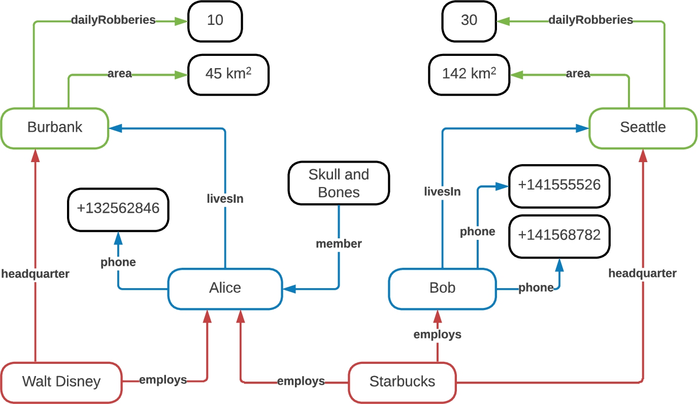
To be able to apply differential privacy to a dataset in the form of an RDF graph, we must thus begin by identifying the different types of entities present in the graph, and the set of individuals in each type. Consider, for instance, the RDF graph  ), two companies (depicted in
  ) and two cities (depicted in
  ). Said otherwise, there are two individuals of each entity type, adding up to six individuals in all. When querying the graph, we will be interested in protecting the contribution of all these individuals, and when applying differential privacy techniques to this end, we will then consider as a neighbor any other graph that differs in the contribution of either of them.
We refer to the semantic information necessary to identify the individuals in an RDF graph
3.1.2.Formal definition
We briefly review some basic RDF terminology following standard notation used in the literature [14,16], where more details can be found. The RDF language assumes the existence of an infinite set U (of URI references), an infinite set B (of blank nodes), and an infinite set L (of RDF literals). An RDF triple is a term of the form
To hint how we can formally define entities within an RDF graph, observe first the six colored sub-graphs identified in Fig. 1: two green, two blue and two red. All have a star shape [1], consisting of a “center” with outgoing and/or incoming edges, i.e. predicates. Sub-graphs representing individuals of the same entity type are built from the same set of predicates. For example, both (blue) sub-graphs, representing people, are built from predicates
Definition 4
Definition 4(Star BGP).
A BGP is called a star if
1. both the subject and the object of all its triple patterns are variables,
2. all triple patterns have different predicates, and
3. it consists of either
(a) a single triple pattern with no join vertex, i.e. a triple pattern whose subject and object are distinct variables, or
(b) multiple triple patterns with a single join vertex, which appears once and only once in every triple pattern
Example 3.1
Example 3.1(Star BGP).
The three stars employed to identify the different entities in our running example (Fig. 1) are (modulo variable renaming): 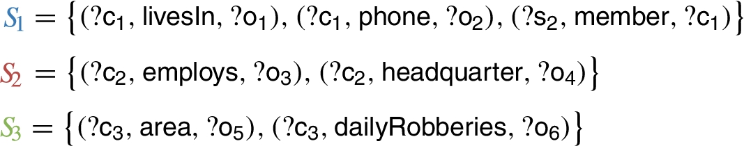
Note that in each  ,
,  and
and  . Formally, we define the center of a star as the join vertex if the star contains multiple patterns, or the variable appearing in the subject of the triple pattern in case it consists of a single triple pattern.33 We say that a set of stars is pairwise predicate-disjoint (or simply pairwise disjoint when no ambiguity arises), if no pair of stars in the collection share a common predicate. They thus define what we call a differential privacy schema:
Definition 5
Definition 5(Dp-schema).
A differential privacy schema (dp-schema, for short)
The set  is a dp-schema. as well as its sub-set
 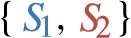 . However, this second schema falls short of describing the whole graph
Definition 6
Definition 6(Induced sub-graphs).
Let
Example 3.2
Example 3.2(Induced sub-graph).
The star  induces two sub-graphs
  and
and  over
over 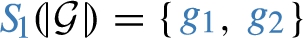 . These correspond to the blue sub-graphs in Fig. 1, which are formally defined as:
Likewise,  , where
Intuitively, the set of induced sub-graphs  , but it is not materialized in
  . From the privacy point of view, the values of the star center are the unique identifiers of the entities contributing the data in each sub-graph, and their values must be kept confidential.
The notion of induced sub-graphs naturally extends from single stars, to dp-schemas, i.e. sets of stars. Concretely, we let  .
.
Now we have all the prerequisites to define the core concept of this section:
Definition 7
Definition 7(Dp-schema compliance).
We say that an RDF graph
Example 3.3
Example 3.3(Dp-schema compliance).
Our running example  . In contrast, it does not comply with dp-schema
  .
.
In summary, if a graph
3.1.3.Discussion
We now address a few key points about dp-schemas.
No shared attribute between entities At first sight, the requirement that stars in a dp-schema be predicate pairwise disjoint might seem a limitation, as it requires that each attribute belong to a single entity type. For instance, it might seem natural to consider that predicate  (which identifies companies) and
  (which identifies people). However, for the sake of protection it makes no difference to which star it belongs, since our application of differential privacy will protect the contribution of all individuals, regardless of its type.
Existence of dp-schemas RDF graphs always admit compliant dp-schemas. In particular, every graph complies with a trivial dp-schema comprising the union of all singleton BGP’s of the form
Compliance verification Checking whether an RDF graph complies with a given schema
Dp-schema provision For practical purposes, we assume that the database administrator of the RDF graph at stake is responsible for designing the dp-schema the graph shall comply with, and for ensuring the compliance as the graph evolves. In this latter regard, observe that removing an RDF triple from the graph always preserves the dp-schema compliance, and adding a triple also preserves compliance provided the predicate in the triple already appears in the dp-schema. We believe this is a natural assumption, as in the relational data model this would correspond to changing the schema of the database by adding a new attribute to a relation if the new predicate is incorporated into an existing star of the dp-schema or creating a new table if the predicate is added to the dp-schema as a new star.
3.2.Predicate multiplicity
Automatic approaches to answer dataset queries in a differentially private manner are typically obtained by adding noise to the query results, calibrated according to their sensitivity. Thus, a prerequisite to apply differential privacy to counting queries over RDF graphs is that they have bounded sensitivity. Unfortunately, this does not occur in the general case.
To see this, consider graph  ) is replaced by somebody else’s contribution. The query answer over this neighboring graph can certainly be any integer
This problem arises because of the presence of predicates that are not one-to-one. To recover bounded sensitivities, we have to restrict ourselves to predicates that have bounded multiplicity. For instance, if the administrator of graph
On the formal level, we associate such bounds to triple patterns rather than to predicates. This is because in the presence of compliant dp-schemas, predicates are identified with triple patterns (every predicate within a dp-schema occurs in a single triple pattern, in a single star).
Definition 8
Definition 8(Triple-pattern multiplicity).
Let
Many predicates (or equivalently, triple patterns) would have a natural multiplicity bound of 1. For instance, a city has a unique
Henceforth, in the remainder we assume the system administrator provides a dp-scheme
For bounding the local sensitivity of queries in Section 5, it will suffices a coarser notion of multiplicity, at the level of stars rather than triple patterns. The required generalization is straightforward:
Definition 9
Definition 9(Star multiplicity).
Let
Example 3.4
Example 3.4(Star multiplicity).
Assume that a graph administrator adopts dp-schema  and requires that each individual
  will have multiplicity
  .
.
4.Queries
In this section we describe the subset of queries over RDF graphs for which we provide differential privacy, and show how dp-schemes enable a decomposition result for the evaluation of such queries.
4.1.Supported queries
We develop differential privacy for counting queries over the SPARQL fragment of basic graph patterns with filter expressions, also known as constrained basic graph pattern (CBGP) [1]. In this fragment, a query is denoted by a pair
For simplicity, we consider only CBGPs that are semantically valid. We also assume that in a graph
Example 4.1.
Take RDF graph  . Now assume we want to know how many people have a coworker in a company with headquarters in a city with over 20 daily robberies? The query can be cast in terms of the CBGP
Triple patterns in an RDF graph compliant with a dp-schema
 which contains the triple pattern
Finally, a user query is a CBGP
1.
2.
3.
Example 4.2.
The query from the previous example can be expressed as
4.2.Evaluation decomposition
Continuing with the previous example, assume we want to evaluate B (from Example 4.1) over  induces on
Hence, for any query
1. every
2. for any two triple patterns
Example 4.3.
For the CBGP from Example 4.1, B is split into four elementary BGPs by dp-schema  , i.e.
  , but they are consireded different elementary BGPs because they share predicate
  and
and  , respectively.
If B were extended, e.g. , with triple pattern
 , but remain different members of
  .)
.)Note also that the elementary BGP where a triple pattern belongs to is determined by the center of the triple pattern, all triple patterns in the same split must share the same variable or RDF term as their center. The interest in
Lemma 2.
If
Then, following the terminology defined in [29] for joins between multisets of solution mappings, we can extend the lemma to B as follows:
Lemma 3.
We have already observed that
We are now in a position to establish differential privacy for SPARQL count and histogram queries.
5.Towards differential privacy for SPARQL
In this section we develop all the prerequisites to extend Lemma 1 from the relational model to the graph model, in terms of the
5.1.Preliminary notions
We begin defining the notion of size and distance between RDF graphs. These are straightforward adaptations of the relational case, where the induced sub-graphs play the role of table rows. Concretely, the size of a graph refers to the number of individuals present in it. Formally, given an RDF graph
Moreover, we say that two graphs are k far apart if one can be obtained from the other by replacing k of its induced sub-graphs. Formally, given a pair of RDF graphs
Finally, this notion of distance between RDF graphs readily induces a notion of local sensitivity (at distance k)
In order not to clutter the presentation, we usually omit the underlying dp-schema when referring to the size of an RDF graph, the distance between a pair of RDF graphs, and the local sensitivity of a
5.2.Elastic sensitivity
Our next step is, given a user query Q and an RDF graph
To this end, observe that the naive approach of evaluating the query on every neighbor (at distance k) of
In the remainder of the section we adapt Johnson et al.’s approach to the case of RDF graphs and
In our case, these transformations are given by the CBGP of user queries, more concretely, by their BGP part. We thus introduce the auxiliary notion of BGP elastic stability. A key property of this notion is that it allows bounding the local sensitivity of counting queries: Given a BGP B, its elastic stability at distance k with respect to a graph
The formal definition of elastic stability relies on the frequency of most popular values. More precisely, if
The counting on the latter query will be greater than (or equal to) the one on the former query and, therefore, a valid (possibly looser, though) upper bound for
To compute the elastic stability of BGP B at distance k of graph
Base case: If
Inductive case: If
The intuition behind the base case is easy to grasp. For
We are now ready to define the elastic stability of a BGP B at distance k of graph
Base case: If
Inductive case: If
If the covering star S of
As so defined, the local stability bounds the local sensitivity of counting queries:
Lemma 4.
For any CBGP query
The main intuition behind the proof is that changes made to a graph to get a new graph at distance 1, are limited to a sub-graph
Proof.
The proof of this lemma follows the same strategy as the proof in [19, Lemma 2], and is by induction on the length of
– Case
since the local sensitivity at distance k is calculated as the max of the sensitivities of all graphs at distance 1 of all graphs at distance k or less of– Case
We chose the largest of the two values when calculating1. When
2. In the symmetric case, when
Now we have all the prerequisite to define the elastic sensitivity of user queries (at fixed distances of a given graph):
And as in Johnson et al. [19], the above lemma readily leads us to the desired bound for (the three kind of) user queries:
Lemma 5.
For any user query Q, and any graph
Proof.
By case analysis on the type of user query Q:
– For plain counting queries (
– For plain unique counting queries (
– For counting queries after grouping (
Lemma 5 readily establishes our main result, which allows applying differential privacy to
Theorem 3.
Assume that our universe of (valid) RDF graphs is composed by the graphs that comply with dp-schema
The theorem follows immediately from Theorem 2 and Lemmas 1 and 5.
6.Evaluation
Having characterized formally how an algorithm can be implemented to enforce differential privacy on SPARQL queries based on privacy schemes, in this section, we present an empirical evaluation of how the algorithm would behave in real scenarios.
Setup We conducted our evaluation on a 2018 Macbook Pro with 16 GB of RAM memory having installed a Fuseki instance on a 2 AMD Opteron server with an SSD drive and 64 GB of RAM memory. We used Java 1.17 to implement our proof of concept. We also used the SecureRandom Java class to generate the random numbers to calculate the Laplacian probability distribution since that class implements a well-tested random number generator,55 an essential component for ensuring the correctness of our privacy guarantees algorithm. The code and all the queries used for this evaluation are available in GitHub.66
Data In the evaluation we used real world data and queries from Wikidata [34]. Wikidata is a collaboratively edited knowledge base hosted by the Wikimedia Foundation. It is a common source of data for Wikimedia projects such as Wikipedia, and it has been made available to the general public under a public domain license. Wikidata stores 86,671,701 items (RDF resources), and 1,084,935,969 statements (triples77). We selected a subset of the Wikidata Truthy from 2021-06-23, which has all but direct properties (i.e. http://www.wikidata.org/prop/direct/P*) removed [18,35]. The data is available to download from Google Drive.88 We also provide the scripts to generate this Wikidata version in our Github repository.99 We use the following prefixes from Wikidata along this section: 
6.1.Privacy schema
Our dp-schema is defined based on three pairwise disjoint stars,
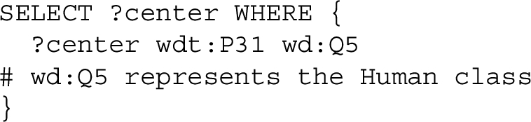
This gathers the instances of the class Human. Star instances were formed by selecting a subset of properties of the three classes using star queries centered in the URIs (each instance representing either a Human, an Organization or a Profession) to define three sub-graphs covered by three stars,
Evaluation privacy schema The three stars employed to identify the different entities in our evaluation schema are (modulo variable renaming):
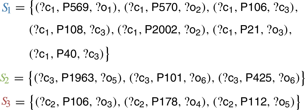
These three stars shouldn’t be used directly as a privacy schema because
The Wikidata properties that allow joining data from two different stars are P108 Employer from Humans to Organizations, P106 Profession from Humans to Professions, P106 Occupation from Organizations to Professions and P112 Founded by from Organizations to Humans. Table 1 shows statistics about the instances of the stars in our data, including star size (on top of the table).
Table 1
Table showing key statistics about the data in our privacy schema (the largest schema is by far the Humans star)
| Humans: 9,181,487 | ||||
| P569 | P570 | P106 | P108 | P2002 |
| 5,109,648 | 2,511,719 | 6,446,811 | 1,085,617 | 159,194 |
| P21 | P40 | |||
| 7,223,891 | 707,747 | |||
| Professions: 7,786 | ||
| P1963 | P101 | P425 |
| 97 | 95 | 3,018 |
| Organizations: 72,879 | ||
| P106 | P178 | P112 |
| 50 | 16 | 2,789 |
6.2.Queries
We selected 26 queries from the query logs in [18,35] containing the predicates used in our dp-schema. Since the amount of COUNT queries in the query logs is small [4] for each of these queries we added the COUNT keyword and we removed the triples from the query that were not accessing our schema. In addition, these queries were modified to get a diverse set of query results and types.
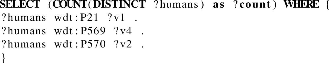
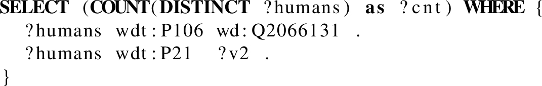
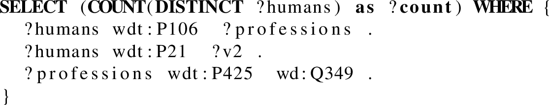
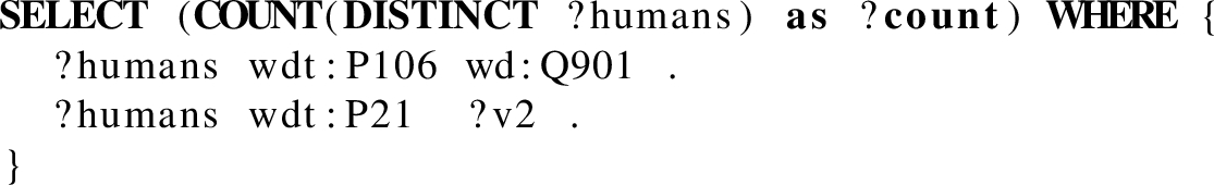
We consider star queries which are queries covered by a single star from the dp-schema. These queries can only add filters and remove triple patterns from the star. Therefore, a star query is centered around a single join vertex
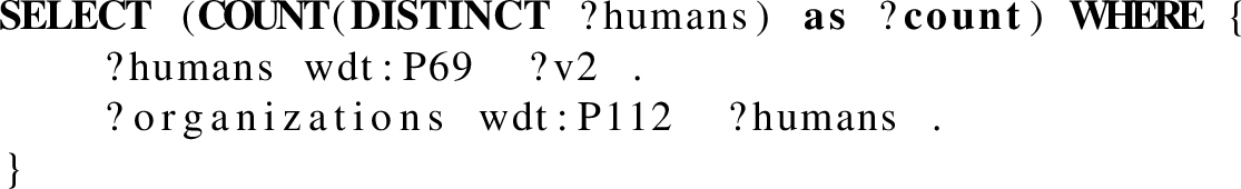
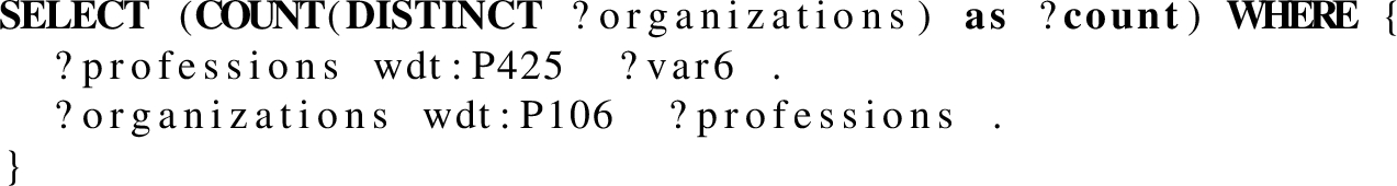
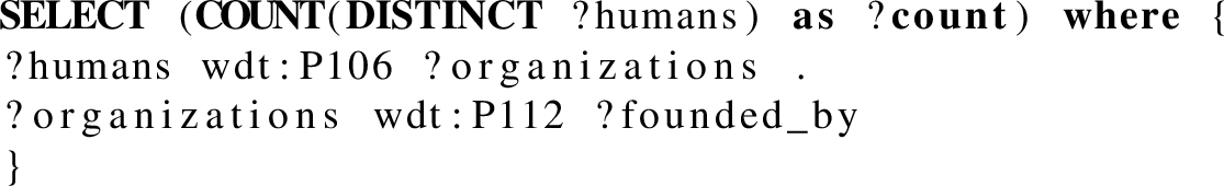
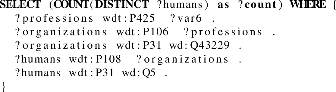
Fig. 2.
Star-shaped query
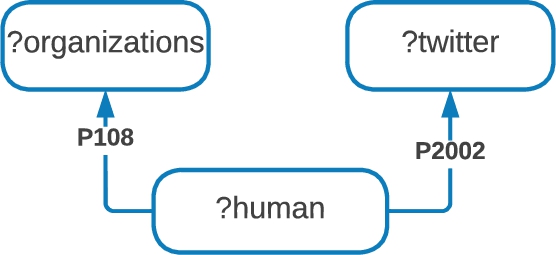
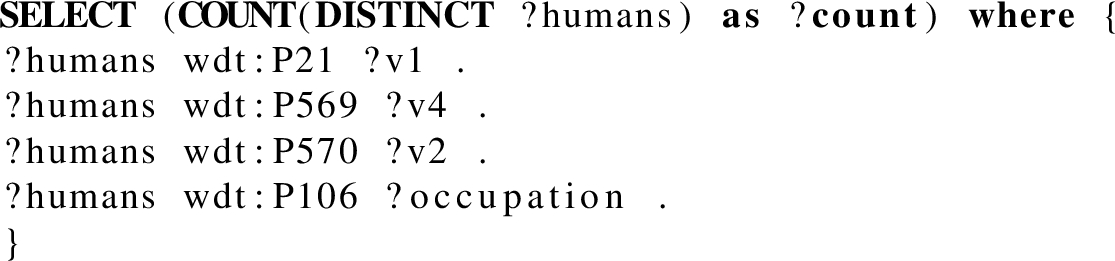
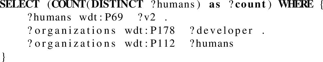
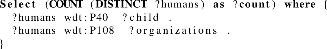
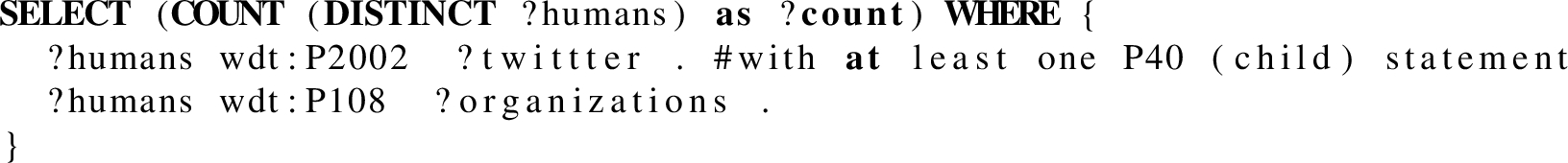
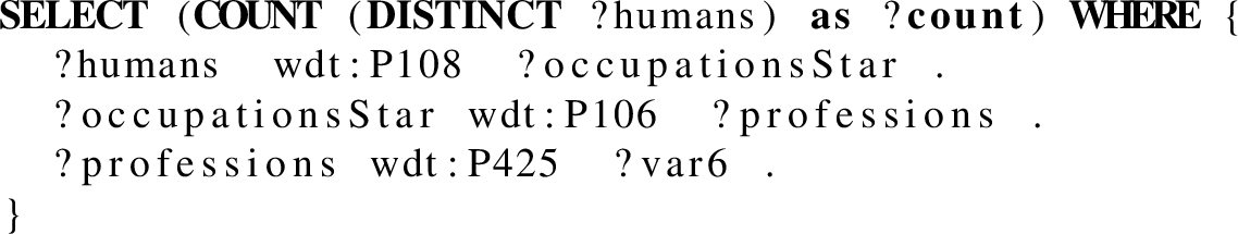
Fig. 3.
Linear query

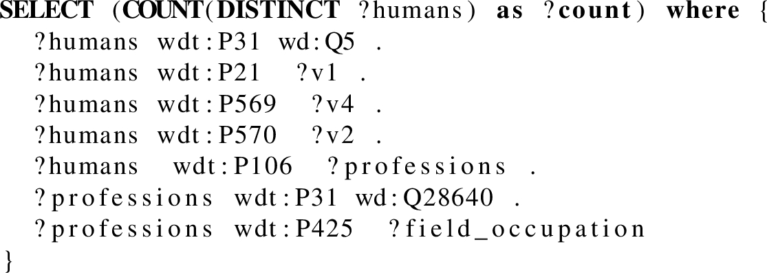
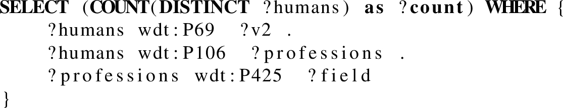
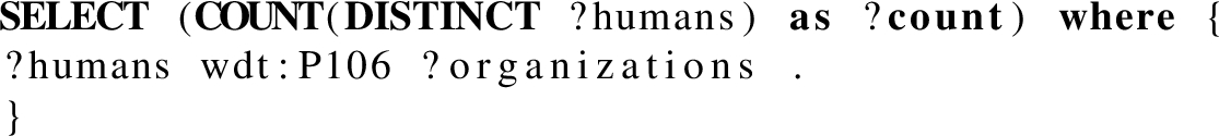
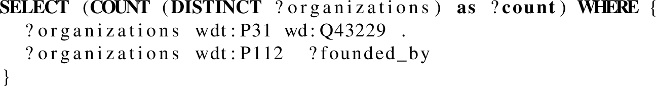
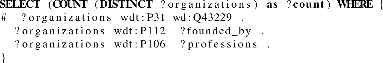
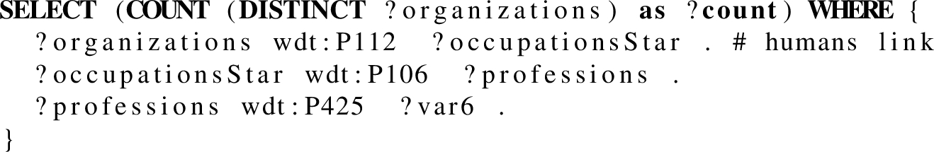
Fig. 4.
Snowflake query
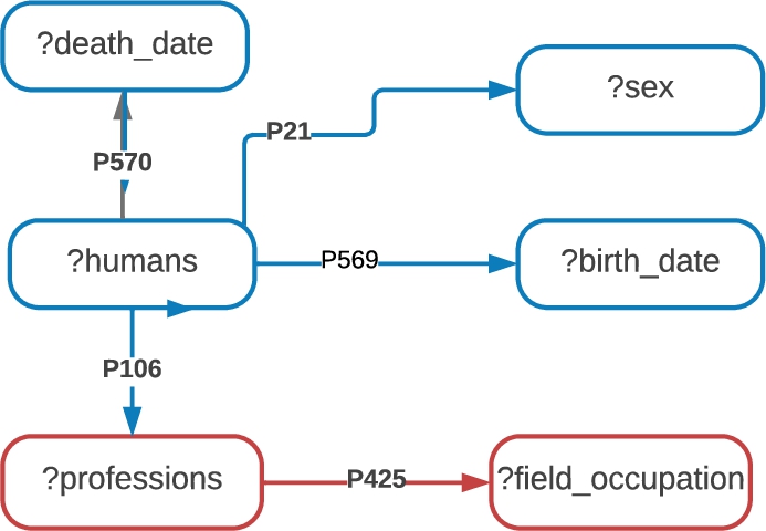
Table 2
Results of the execution of Wikidata queries using our differential privacy method. Those queries with sensitivity “1.0” are star queries since the sensitivity of a COUNT query over a single star schema is 1 (a COUNT query over a table), and their elastic stability is “x” as described in Section 5.2 if there are joins between star BGPs, the sensitivity increases based on the stability polynomial, calculated according to Theorem 3
| Query ID | Actual result | Average private | Average private | Sensitivity | Stability |
| result using | result using | ||||
| Epsilon = 0.1 | Epsilon = 1.0 | ||||
| Q1 | 2,275,177 | 2,275,176 | 2,275,176 | 1.0 | 1 |
| Q2 | 1,717,945 | 1,717,940 | 1,717,945 | 1.0 | 1 |
| Q3 | 1,274,788 | 1,189,636 | 1,270,649 | 290,415 | (x+290,863) * 1 |
| Q4 | 17,440 | 17,464 | 17,319 | 245 | (x+18) * 1 |
| Q5 | 86 | 110.8 | 203.1 | 245 | (x+18) * 1 |
| Q6 | 1,170,315 | 3,860,469 | 1,137,687 | 400,363 | (x+400,981) * 1 |
| Q7 | 3,018 | 3019 | 3,017 | 1.0 | 1 |
| Q8 | 50 | 57 | 50 | 1.0 | 1 |
| Q9 | 31 | 1577 | 37 | 241.3 | (x+8) * 1 |
| Q10 | 14,477 | 14,472 | 14,477 | 1.0 | 1 |
| Q11 | 2,789 | 2,792 | 2,789 | 1.0 | 1 |
| Q12 | 221 | 1,144 | 89 | 1,162.2 | (x+1,164) * 1 |
| Q13 | 6,446,811 | 6,446,812 | 6,446,810 | 1.0 | 1 |
| Q14 | 3,615 | 3,613 | 3,614 | 1.0 | 1 |
| Q15 | 0 | 71 | 8 | 250.8 | (x+33) * 1 |
| Q16 | 21,683 | 21,682 | 21,682 | 1.0 | 1 |
| Q17 | 2,789 | 2,788 | 2,788 | 1.0 | 1 |
| Q18 | 25 | 465 | 34 | 248.5 | (x+27) * 1 |
| Q19 | 865 | 864 | 865 | 1.0 | 1 |
| Q20 | 7 | 7,087,181 | 44,254 | 1,656,501 | (x+6,189) * (x+8) * 1 |
| Q21 | 3,213 | 1,739,549 | 31,357 | 1,651,883 | (x+6) * (x+6,189) * 1 |
| Q22 | 2,092 | 377,638,493 | 1,600,610 | 408,594,207 | (x+7) * (x+1,694,747) * 1 |
| Q23 | 23,450 | 23,449 | 23,449 | 1.0 | 1 |
| Q24 | 2,626 | 1,071,418 | 231,278 | 628,018 | (x+628,987) * 1 |
| Q25 | 29,352 | 1,593,488 | 42,317 | 628,018 | (x+628,987) * 1 |
| Q26 | 29,352 | 29,350 | 29,351 | 1.0 | 1 |
6.3.Results
We report the results of our evaluation in Table 2, showing the actual count output by the queries and the average result to these queries with added noise (calculated applying the method described in Section 5). We followed the query schema introduced in Section 5.2, that uses the BGP part of each query to calculate the initial most popular values (mpv). We report the results using two values for ϵ, 0.1 and 1.0. We also report the median error percentage for
(Blue) squares in Fig. 5 represent star queries (typically accessing a single star within the dp-schema), have a very low error (and thus a high utility) compared to the other two types of queries that involved at least one “join” operation across stars.
However, the smaller the result from the COUNT, the larger the error introduced. (Red) triangles represent path queries and thus queries with join operations. Only query
Fig. 5.
This plot shows that star-shaped queries (blue squares) have the greatest utility, since they are likely not to have joins between stars in the schema. It also shows that queries accessing large amounts of data have high utility. Notice that
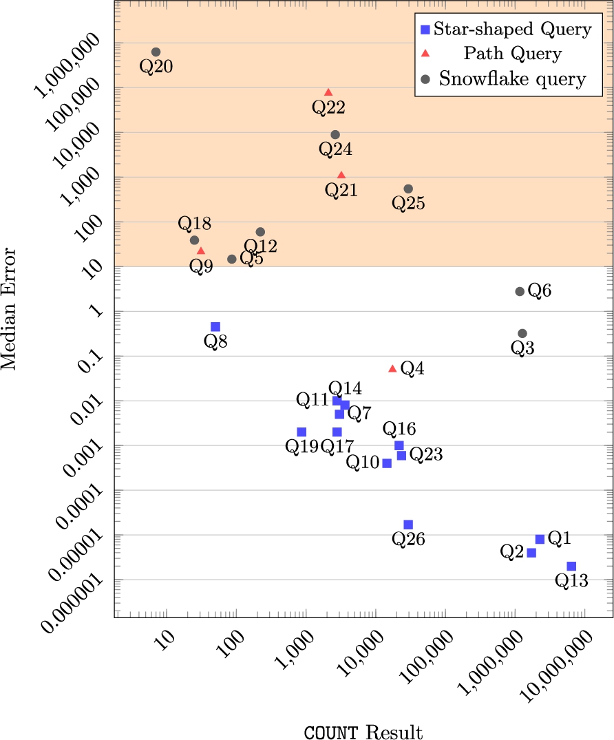
The sensitivity and stability columns in Table 2 clearly show that the larger the degree in the stability polynomial the greater the query sensitivity, and thus, the higher the error in the result. Note that in most cases the derived queries produce smaller results than the simpler queries, thus the errors are larger. The only queries where this is not the case are queries
7.Related work
The study of how to guarantee the privacy of individuals contributing personal data to datasets is a long studied problem. In this work we have focused on how to guarantee this privacy in RDF data graphs accessed through SPARQL queries using differential privacy. The related work can be roughly classified into those that provide some privacy guarantees to accesses to data stored in (social) graphs and those that guarantee privacy over the results returned by SPARQL queries. We briefly look over these works in this section.
7.1.Privacy over SPARQL
There have been several approaches to address privacy concerns related queries to RDF data. A good survey can be found in [32]. There is a basic anonymization protection that a SPARQL engine must provide to queries that directly return individuals, as opposed to aggregated data. Similar to the case of relational databases where attribute values are anonymized using nulls, the work presented in [13] uses blank nodes to hide sensitive data. Delanoux et al. [7] introduce a more general framework with formal soundness guarantees for privacy policies that describe information that should be hidden as well as utility policies that describe information that should be available. The framework checks whether policies are compatible with each other, and based on a set of basic update queries that use blank nodes and deletions of triples, automatically derives from the policies candidate sets of anonymization operations that guarantee to transform any input dataset into a dataset satisfying the required policies. However, their soundness guarantees do not imply any formal privacy guarantees. Two early methods developed for privacy protection when answering queries about classes in a dataset are k-anonymity and l-diversity. In particular, k-anonymity is used in [17,31] to answer queries in RDF datasets. Unfortunately, it is well-known these methods, in contrast to differential privacy, do not provide formal guarantees for privacy.
The only work known to us that directly applies differential privacy to SPARQL queries is [32]. But surprisingly, differential privacy is realized through local sensitivity alone without the use of a smoothing function necessary for correctness [12]. A privacy-preserving query language for RDF streams is introduced in [8]. Limiting queries to that language servers can continuously release privacy-preserving histograms (or distributions) from online streams. Han et al. [15] provide differentially-private variants of the algorithms TransE and RESCAL, aimed at constructing knowledge graph embeddings in the form of real-valued vectors. While the authors show that these encodings allow performing some analyses with a reasonable privacy-utility tradeoff, inlcuding clustering and link prediction, it is an open question whether this generalizes to further analyses or counting queries as addressed in the current article.
7.2.Privacy in social graphs
A central task to the development of any practical differentially private analysis tool is finding appropriate approximations and alternatives to global sensitivity: it should be easy to calculate, and, at the same time, close enough to the real sensitivity to allow the computation of statistically useful results. A well-known approach is to rely on the concept of restricted sensitivity [3]. Restricted sensitivity is tailored to provide privacy guarantees assuming datasets come from a specific subgroup of the universe of all possible datasets, and it was introduced in the context of social-graph data analysis. There are two natural notions from which one can define adjacency of graphs: differences on edges and differences on vertices. The distance between two graphs,
8.Conclusions
In this paper we have introduced a framework to develop differential privacy tools for RDF data repositories. We have used the framework to develop an
We have implemented our algorithm and tested it using the Wikidata RDF database, queries from its log files and other example queries found at the Wikidata endpoint. The simulations show the approach to be effective for queries over large repositories, such as Wikidata, and in many cases for queries within the 10 of thousands answers to aggregate. However, even though elastic sensitivity has been designed to bind the stability of joins, the sensitivity of a query with joins can still be very high. As in the case of SQL queries in relational databases, in order to keep the noise in SPARQL queries under a single percentage digit, query results should have over 1M tuples and
There are many pending issues to address. We can still apply several optimizations to our framework. For example, public graphs can be treated as public tables. If they participate in joins, we can directly use their most popular result mappings during calculation of the query sensitivity. From the more practical point of view, more operations need to be implemented. We can consider the approaches described in [19] for SQL to add aggregation functions like sum and averages to our framework. There are also issues to consider about the impact that such algorithms will have on SPARQL query engines. From the more formal side, it is still important to keep searching for better approximations of local and global sensitivities as well as alternative definitions that are less onerous than differential privacy. One possibility is to find a way to apply restricted sensitivity to more types of queries by adding more semantic information to a dp-schema. It might also be possible to find a more accurate approximation for the elastic sensitivity of
Notes
1 Calculation of query sensitivity will depend on the domain of blank nodes which can change under different contexts and implementations. This is a topic of future research.
2 The more general definition of triple patterns allows also for variables in the predicate component of triple patterns.
3 The notion of star BGP that we use here is similar to that of star query from [1], except that in a star query the center of the star must always appear as subject.
4 Observe that there might be multiple such triple patterns in B, all of them yielding valid upper bounds for
6 Repository https://github.com/cbuil/DPSparql.
10 Note that this observation suggests a more subtle definition of privacy scheme would be useful.
Acknowledgements
We thank the reviewers for their thorough work revising this paper, which improved the overall quality of the paper. Carlos Buil-Aranda was supported by Fondecyt Iniciacion 11170714 and by ANID – Millennium Science Initiative Program – Code ICN17_002. Jorge Lobo was partially supported by the Spanish Ministry of Economy and Competitiveness under Grant Numbers: TIN-2016-81032-P, MDM-2015-052, and the U.S. Army Research Office under Agreement Number W911NF1910432. Federico Olmedo was also supported by ANID – Millennium Science Initiative Program – Code ICN17_002.
Appendices
Appendix A.
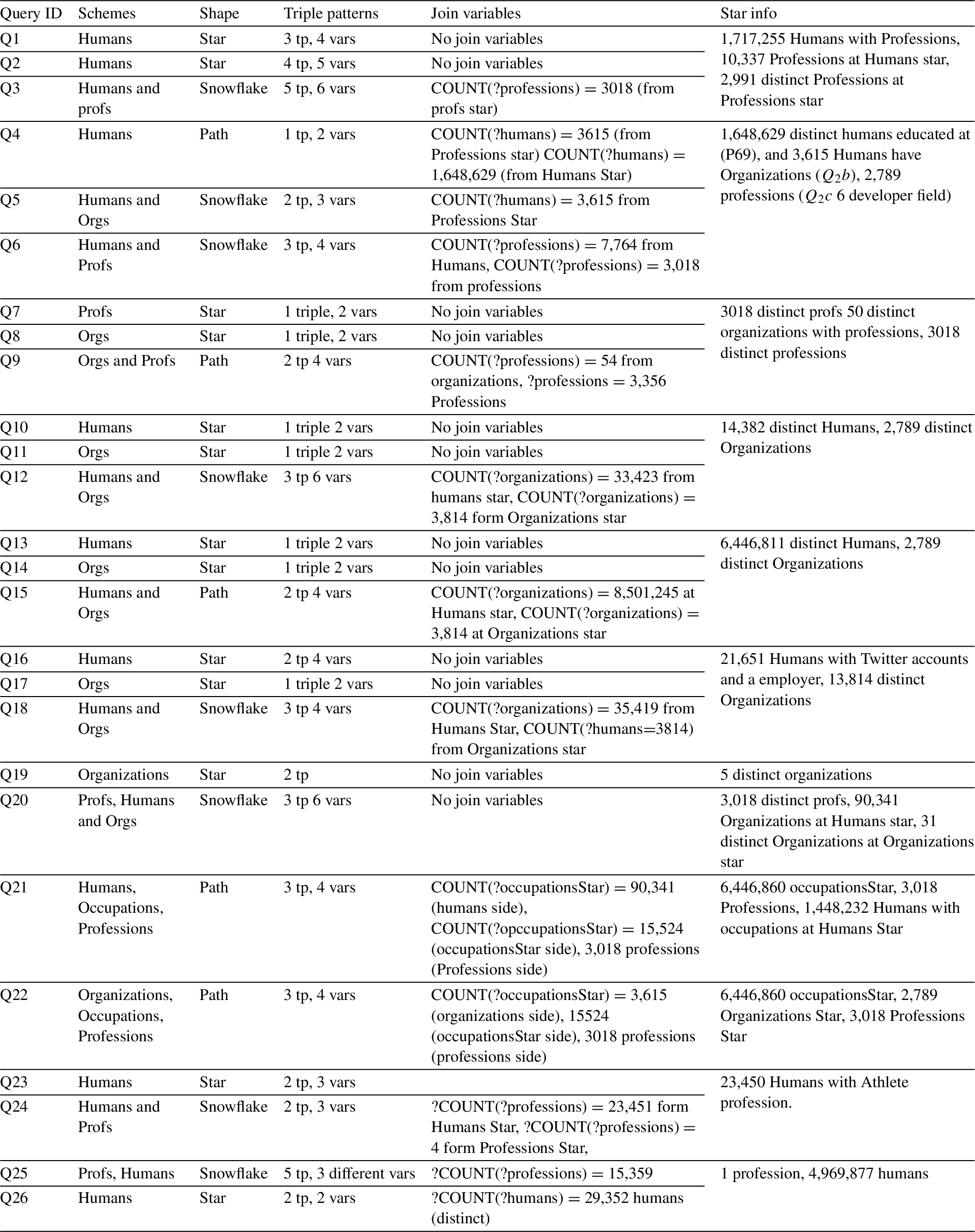
Appendix A.Query characteristics
In this Section we present the characteristics of the queries we used in Section 6. The table presents the query ID (which refer to queries Section B in this Appendix), the stars within the Privacy Schema we defined in 6, the query shape, the amount of tripe patterns in the queries as well as the number of variables, the join variables when applicable, including the amount of mappings for each join variable, and data about the Privacy Schema stars in the query.
Table 3
Table showing the main characteristics of each query to the privacy schema
Appendix B.
Appendix B.Queries
In this Section we present the queries we used in Section 6. There are 11 base queries with several variations, totaling 26 SPARQL COUNT queries.
Query
Query
Query
Query
Query
Query
Query
Query

Query
Query
Query

Query

Query
Query
Query
Query
Query
Query

Query
Query
Query
Query
Query
Query
Query
Query

References
[1] | G. Aluç, O. Hartig, M.T. Özsu and K. Daudjee, Diversified stress testing of RDF data management systems, in: International Semantic Web Conference, Springer, (2014) , pp. 197–212. |
[2] | M. Arapinis, D. Figueira and M. Gaboardi, Sensitivity of counting queries, in: 43rd International Colloquium on Automata, Languages, and Programming, ICALP 2016, July 11–15, 2016, Rome, Italy, I. Chatzigiannakis, M. Mitzenmacher, Y. Rabani and D. Sangiorgi, eds, LIPIcs, Vol. 55: , Schloss Dagstuhl – Leibniz-Zentrum für Informatik, (2016) , pp. 120–112013. |
[3] | J. Blocki, A. Blum, A. Datta and O. Sheffet, Differentially private data analysis of social networks via restricted sensitivity, in: Proceedings of the 4th Conference on Innovations in Theoretical Computer Science, ITCS’13, ACM, New York, NY, USA, (2013) , pp. 87–96. ISBN 978-1-4503-1859-4. doi:10.1145/2422436.2422449. |
[4] | A. Bonifati, W. Martens and T. Timm, Navigating the maze of Wikidata query logs, in: The World Wide Web Conference, (2019) , pp. 127–138. doi:10.1145/3308558.3313472. |
[5] | S. Chen and S. Zhou, Recursive mechanism: Towards node differential privacy and unrestricted joins, in: Proceedings of the 2013 ACM SIGMOD International Conference on Management of Data, ACM, (2013) , pp. 653–664. doi:10.1145/2463676.2465304. |
[6] | R. Cyganiak, D. Wood and M. Lanthaler, RDF 1.1 Concepts and Abstract Syntax, (2014) . |
[7] | R. Delanaux, A. Bonifati, M.-C. Rousset and R. Thion, Query-based linked data anonymization, in: International Semantic Web Conference, Springer, (2018) , pp. 530–546. |
[8] | D. Dell’Aglio and A. Bernstein, Differentially private stream processing for the semantic web, in: Proceedings of the Web Conference 2020, WWW’20, Association for Computing Machinery, New York, NY, USA, (2020) , pp. 1977–1987. ISBN 9781450370233. doi:10.1145/3366423.3380265. |
[9] | C. Dwork, Differential privacy, in: 33rd International Colloquium on Automata, Languages and Programming, Part II (ICALP 2006), Lecture Notes in Computer Science, Vol. 4052: , Springer Verlag, (2006) , pp. 1–12, https://www.microsoft.com/en-us/research/publication/differential-privacy/. ISBN 3-540-35907-9. |
[10] | C. Dwork, Differential privacy: A survey of results, in: International Conference on Theory and Applications of Models of Computation, Springer, (2008) , pp. 1–19. |
[11] | C. Dwork, K. Kenthapadi, F. McSherry, I. Mironov and M. Naor, Our data, ourselves: Privacy via distributed noise generation, in: Annual International Conference on the Theory and Applications of Cryptographic Techniques, Springer, (2006) , pp. 486–503. |
[12] | C. Dwork, A. Roth et al., The algorithmic foundations of differential privacy, Foundations and Trends® in Theoretical Computer Science 9: (3–4) ((2014) ), 211–407. |
[13] | B.C. Grau and E.V. Kostylev, Logical foundations of privacy-preserving publishing of linked data, in: Thirtieth AAAI Conference on Artificial Intelligence, (2016) . |
[14] | C. Gutierrez, C. Hurtado and A.O. Mendelzon, Foundations of semantic web databases, in: Proceedings of the Twenty-Third ACM SIGMOD-SIGACT-SIGART Symposium on Principles of Database Systems, (2004) , pp. 95–106. doi:10.1145/1055558.1055573. |
[15] | X. Han, D. Dell’Aglio, T. Grubenmann, R. Cheng and A. Bernstein, A framework for differentially-private knowledge graph embeddings, J. Web Semant. 72: ((2022) ), 100696. doi:10.1016/j.websem.2021.100696. |
[16] | S. Harris and A. Seaborne, (2012) , SPARQL 1.1 Query language, W3C recommendation, http://www.w3.org/TR/2010/WD-sparql11-query-20101014/. |
[17] | B. Heitmann, F. Hermsen and S. Decker, k – RDF-neighbourhood anonymity: Combining structural and attribute-based anonymisation for linked data, in: PrivOn ISWC, (2017) . |
[18] | A. Hogan, C. Riveros, C. Rojas and A. Soto, A worst-case optimal join algorithm for SPARQL, in: The Semantic Web – ISWC 2019 – 18th International Semantic Web Conference, Auckland, New Zealand, October 26–30, 2019, Proceedings, Part I, C. Ghidini, O. Hartig, M. Maleshkova, V. Svátek, I.F. Cruz, A. Hogan, J. Song, M. Lefrançois and F. Gandon, eds, Lecture Notes in Computer Science, Vol. 11778: , Springer, Auckland, New Zealand, (2019) , pp. 258–275. doi:10.1007/978-3-030-30793-6_15. |
[19] | N. Johnson, J.P. Near and D. Song, Towards practical differential privacy for SQL queries, Proceedings of the VLDB Endowment 11: (5) ((2018) ), 526–539. doi:10.1145/3187009.3177733. |
[20] | D. Kifer and A. Machanavajjhala, No free lunch in data privacy, in: Proceedings of the 2011 ACM SIGMOD International Conference on Management of Data, SIGMOD’11, ACM, New York, NY, USA, (2011) , pp. 193–204. ISBN 978-1-4503-0661-4. doi:10.1145/1989323.1989345. |
[21] | N. Li, T. Li and S. Venkatasubramanian, t-Closeness: Privacy beyond k-anonymity and l-diversity, in: Data Engineering, 2007. ICDE 2007. IEEE 23rd International Conference on, IEEE, (2007) , pp. 106–115. |
[22] | N. Li, W. Qardaji, D. Su, Y. Wu and W. Yang, Membership privacy: A unifying framework for privacy definitions, in: Proceedings of the 2013 ACM SIGSAC Conference on Computer & Communications Security, ACM, (2013) , pp. 889–900. |
[23] | A. Machanavajjhala, J. Gehrke, D. Kifer and M. Venkitasubramaniam, l-Diversity: Privacy beyond k-anonymity, in: 22nd International Conference on Data Engineering (ICDE’06), IEEE, (2006) , pp. 24–24. doi:10.1109/ICDE.2006.1. |
[24] | F.D. McSherry, Privacy integrated queries: An extensible platform for privacy-preserving data analysis, in: Proceedings of the 2009 ACM SIGMOD International Conference on Management of Data, ACM, (2009) , pp. 19–30. doi:10.1145/1559845.1559850. |
[25] | L. Menand, Why do we care so much about privacy?, The New Yorker XCIV(17) ((2018) ), 24–29. |
[26] | R. Motwani and P. Raghavan, Randomized algorithms, ACM Computing Surveys (CSUR) 28: (1) ((1996) ), 33–37. doi:10.1145/234313.234327. |
[27] | K. Nissim, S. Raskhodnikova and A. Smith, Smooth sensitivity and sampling in private data analysis, in: Proceedings of the Thirty-Ninth Annual ACM Symposium on Theory of Computing, STOC’07, ACM, New York, NY, USA, (2007) , pp. 75–84. ISBN 978-1-59593-631-8. doi:10.1145/1250790.1250803. |
[28] | K. Nissim, S. Raskhodnikova and A. Smith, Smooth sensitivity and sampling in private data analysis, 2011, Draft full version v1.0, http://www.cse.psu.edu/~ads22/pubs/NRS07/NRS07-full-draft-v1.pdf. |
[29] | J. Pérez, M. Arenas and C. Gutierrez, Semantics and complexity of SPARQL, TODS 34: (3) ((2009) ), 16. |
[30] | D. Proserpio, S. Goldberg and F. McSherry, Calibrating data to sensitivity in private data analysis: A platform for differentially-private analysis of weighted datasets, Proceedings of the VLDB Endowment 7: (8) ((2014) ), 637–648. doi:10.14778/2732296.2732300. |
[31] | F. Radulovic, R. García Castro and A. Gómez-Pérez, Towards the Anonymisation of RDF Data, (2015) . |
[32] | R.R.C. Silva, B.C. Leal, F.T. Brito, V.M. Vidal and J.C. Machado, A differentially private approach for querying RDF data of social networks, in: Proceedings of the 21st International Database Engineering & Applications Symposium, ACM, (2017) , pp. 74–81. doi:10.1145/3105831.3105838. |
[33] | L. Sweeney, k-Anonymity: A model for protecting privacy, International Journal of Uncertainty, Fuzziness and Knowledge-Based Systems 10: (05) ((2002) ), 557–570. doi:10.1142/S0218488502001648. |
[34] | D. Vrandečić and M. Krötzsch, Wikidata: A free collaborative knowledgebase, Communications of the ACM 57: (10) ((2014) ), 78–85. doi:10.1145/2629489. |
[35] | D. Vrgoc, C. Rojas, R. Angles, M. Arenas, D. Arroyuelo, C.B. Aranda, A. Hogan, G. Navarro, C. Riveros and J. Romero, MillenniumDB: A persistent, open-source, graph database, CoRR ((2021) ), arXiv:2111.01540. |


