
Data journeys: Explaining AI workflows through abstraction
Abstract
Artificial intelligence systems are not simply built on a single dataset or trained model. Instead, they are made by complex data science workflows involving multiple datasets, models, preparation scripts, and algorithms. Given this complexity, in order to understand these AI systems, we need to provide explanations of their functioning at higher levels of abstraction. To tackle this problem, we focus on the extraction and representation of data journeys from these workflows. A data journey is a multi-layered semantic representation of data processing activity linked to data science code and assets. We propose an ontology to capture the essential elements of a data journey and an approach to extract such data journeys. Using a corpus of Python notebooks from Kaggle, we show that we are able to capture high-level semantic data flow that is more compact than using the code structure itself. Furthermore, we show that introducing an intermediate knowledge graph representation outperforms models that rely only on the code itself. Finally, we report on a user survey to reflect on the challenges and opportunities presented by computational data journeys for explainable AI.
1.Introduction
Artificial intelligence systems are widely used and deployed, for example, to make recommendations, answer questions, and help make decisions [70]. The importance of these systems has led to calls for greater transparency and accountability. For example, the ACM Principles for Algorithmic Transparency and Accountability [3] emphasises the need for awareness, audibility, data provenance, and explanation of algorithms particular for predictive models. To address these concerns, the area of Explainable AI (XAI) [9] has emerged.
While much of the XAI literature has focused on the need to explain the outcomes of machine learning and specifically deep learning models [9], a new line of work has begun to emphasise the need to explain how systems are built and trained [6,24,60]. This is because any biases in the training data or data preparation can have significant down stream impacts [60,71]. Indeed, studies of machine learning practitioners have emphasised their need to be able to understand the entire data science workflow in order to intervene effectively [27]. As [27] identified, data scientists, developers, product owners are key target audiences for explainable AI systems to support them in adding new functionality, debugging AI systems, auditing, and understanding when an AI system can be repurposed (i.e. transferability [28,40]). Our work is positioned in this line of research. Specifically, we aim to help explain complex data science and machine learning workflows by providing an abstract representation of them. We follow an “explanation-by-exploration” approach [47], which enables users to obtain an abstract view of the journey of data through an AI workflow and then dive into the code corresponding to those steps. Fortunately, the Semantic Web community has developed a variety of knowledge representation formalisms to capture fundamental elements of data science workflows, such as provenance, data flows, and high-level activities [33,45,52,62]. That being said, data science workflows are complex and, although models and techniques for representing code as a data graphs exist [2,18], generating high-level, compact representations automatically is still an open and challenging problem.
Hence, this article focuses on extracting and representing data journeys, specifically from data science and AI workflows. Inspired by work in data studies, and particularly Leonelli [36,37], we define a data journey as a multi-layered, semantic representation of a data processing activity, linked to the digital assets involved (code, components, data). We propose an ontology for data journeys to capture the essential elements of data science pipelines and explain them in terms of a graph of high-level activities. This sort of high level representation can be useful, for example, to communicate the global view of how an AI system works, audit large code bases of AI systems, identify areas in a code base that can explain how an AI system preprocesses its data and chooses hyperparameters, or to help understand when a particular system can or cannot be employed. Indeed, similar abstract representations of a data flow have been used to perform data debugging [25], to extract common motifs in workflows [22], to determine the provenance of data [48], reason on the relation between policies and process [16], and to support transparency in clinical analysis [5]. Thus, our work aims to bring these benefits to XAI by: (a) producing a definition of data journey that can be supported computationally, and a first ontology that reflects such definition; (b) effectively extracting representations of data journeys from data science pipelines. Our methods do so without the need to execute the pipeline itself, which allows for data journeys to be constructed for many pipelines to facilitate exploration and comparison of how they work.
In this article we demonstrate that we can capture high-level semantic data flow that is more compact than using the code structure itself. Furthermore, we show that introducing an intermediate graph representation of the data flow outperforms models that rely only on the code itself.
Summarising, the contributions of the article are as follows:
– a definition of data journey suitable for computational approaches;
– an ontology for representing data journeys, mapped to existing, state of the art, relevant ontologies;
– an approach for knowledge extraction from Python-based notebooks to generate a compact, high-level explanation of the data journey;
– experiments demonstrating how a graph-based representation of the data science code outperforms one based on the code syntax in a machine learning pipeline supporting the extraction process.
The rest of the article is structured as follows. We begin with a discussion of related work (Section 2). Next, we look at our definition of a data journey and the associated ontology (Section 4). In Section 5, we detail our approach for knowledge extraction. We report on the application of the method and its evaluation in Section 6. Finally, we report on a user survey to discuss the utility of data journeys further (Section 7). We conclude the article reflecting on paths forward for further research (Section 8).
2.Related work
We begin with a discussion of the relevant work in explainable AI. We then detail relevant work that we build upon, specifically: data journeys from social sciences, data provenance, workflow and ontologies for data science, creating knowledge graphs from code, and methods for capturing the data flow from programs.
Explainable AI The larger field of explainable AI has been covered comprehensively by multiple recent surveys [38,43,61,67]. A large amount of this literature is focused on feature-based explanations where the goal is to identify which input features are an important influence an ML model’s output [38]. Examples of such methods include developing approximate simpler explainable models [42,57] (i.e. local explanations) or developing logical representations of models to identify features [32]. While helpful, these sorts of systems do not aim to support explaining the full data science workflow, which, as mentioned, is essential for debugging, auditing, and understanding AI systems [27].
Thus, we focus on explanations that describe the underlying sequence of steps used by the system to arrive at results. These are known as trace-based explanations [12]. As others have argued [65], this is a critical and under-studied area. In this area, the closest work to ours is that on debugging machine learning pipelines [23,24,41,54,59]. These works develop methods for efficiently tracing back to potential sources of poor model performance, unexpected behaviour and, importantly, biases. Our work is different is that we aim to infer high-level representations of the workflow from code instead of instrument executions. Additionally, our aim is to support the idea of explanation by exploration starting from a high-level representation and then diving into the code. We discuss the specific methods we share with these works later in this section.
Data journeys The broad notion of data journeys have been discussed in the data studies literature. In particular, with the recent edited volume by Leonelli and Tempini, which brings together different case studies from plant phenomics to climate data processing and studies them through the lens of data journeys [37]. Fundamentally, they argue that the journey a dataset goes through, its lineage or provenance, is a powerful unit of analysis for explaining it.
Provenance and provenance representations The need to understand the provenance of data has been well documented in the data management [26] and web [44] literature, which has investigated approaches for representing, extracting, querying, and analysing provenance information. Indeed, the importance of understanding provenance for web information led to the W3C Prov standard for provenance interchange [45] as well as the recent Coalition for Content Provenance and Authenticity.11 We refer to the two surveys cited above for more information about provenance systems. Our work, in particular, builds upon these existing representations in order to provide a multi-layered view of a data journey allowing different levels of abstraction to sit alongside one another. Specifically, we build on the notion of datanode as specified in the Datanode Ontology [15], developed to express complex data pipelines to reason upon the propagation of licences and terms and conditions in distributed applications [14].
Workflow abstractions The need to tie data to the workflow that generated it has been recognised in the scientific workflow community [51]. An essential contribution of this work is that, for workflow analytics and reusability, different granularity levels of workflow representations and associated provenance (e.g. high-level tasks in the domain vs command-line tool parameters) should be captured [22,34]. These representations can then be bundled together with the corresponding data assets and other documentation, creating a research object [10] that can be published using web standards [63,64]. However, most data science and machine learning pipelines are not expressed with such workflow formalisms. Instead, data journeys are complementary to these existing definitions and are designed to be extracted from existing code.
Ontologies for representing data science experiments While the aforementioned approaches work for workflow systems where tasks and their dependencies are systematically defined, most applications use flexible programming languages. This is the case for data science methods [66]. There is a body of works on ontologies for representing specific families of data science experiments (surveyed here [61]). In what follows, we select some related work that is either exemplary of the field or relevant to our problem.
OntoDM-core [52] was developed for representing complex data mining activities. Its conceptualisation distinguishing between a design phase, an implementation phase, and an application. As such, its focus is to manage data mining activities as a composite combination of tasks.
The Data Mining Optimisation Ontology (DMOP) [33] aims at classifying the possible data mining approaches and algorithms to support meta-learning through a description of the activities that is implementation-independent. Crucially, it provides concepts to reason over the applicability of different DM methods to certain datasets and their performance on the different tasks. In this work we focus on a different aspect, which is the characterisation of the sequence of operations performed in data science pipeliens, and their summarisation in abstract workflows.
OntoExp [68] was designed to support the annotation of predictive modelling programs in order to support the cataloguing, exploration, and retrieval of collection of experiments according to their high-level features such as the algorithms used for training or the input dataset used.
ML-Schema [56], developed in the context of the W3C Machine Learning Schema Community Group, provides a set of classes and properties to enable the interchange of information about machine learning algorithms, datasets, and experiments.
In this work, we apply the notion of data journeys to support explainable AI and build upon models developed in the scientific workflow communities. Scientific workflows have general properties that are sufficiently portable across different types of AI pipelines. Our proposed ontology generalises over ML-specific ontologies, particularly ML-schema, and therefore can support a broader set of use cases, while still being extendable for more specialised cases.
Finally, the ontologies surveyed are not designed for AI explainability per se but to support search through catalogues of experiments. Instead, data journeys is about explaining AI experiments themselves through exploring the code that implement them. In addition, data journeys are conceived as multi-layered, open-ended objects. Therefore, our proposed layers can be expanded to incorporate other perspectives, like the ones discussed above.
Knowledge graphs from code There are a number of studies that look at extracting knowledge graph representations from code [1,8,11]. CodeOntology [8] aims at translating source code into RDF for supporting expressive queries over source code published as Linked Data. Likewise, GraphGen4Code [1], is able to generate large scale knowledge graphs from source repositories that reflect code semantics. Broadly, the aim of this line of work is to support development use cases such as program search and code automation. Our work is different in that we aim to not just reflect the code semantics but to learn to map code into a higher level of abstraction that may not be directly reflected in the code itself. In that respect, work on code summarization [4] is relevant. However, the aim of code summarization is to generate textual descriptions of source code instead of mapping to a high level ontology as we do here.
Capturing the dataflow from programs In this article, we argue how a data journey should be linked to the source code in order to effectively support explainability, and that dataflows are essential for understanding the rationale of programs. A variety of work has looked at extracting high-level dataflow-like representations from data science code or logging information. Tessera, for example, has looked at extracting high-level tasks from logs of exploratory data analysis [69]. Furthermore, in work most closely related to ours, researchers have investigated extracting provenance representations from programs’ abstract syntax trees (AST). CodeBreaker constructs a machine-interpretable knowledge graph from program code to support end-user tasks such as code search and recommendation [2]. noWorkflow [48] uses the AST of a program to automatically instrument code during execution to capture provenance. Similarly, mlinspect [25] extracts a provenance representation during the execution of python code. It, however, uses a representation tailored to debugging data science code. ProvenanceCurious [30], and Vamsa [49] also use the python AST, but instead of instrumenting at runtime, they use static analysis to infer a provenance graph. We adopt a similar approach of using static analysis. However, unlike these approaches, we use a hybrid method based on knowledge engineering and machine learning to infer high-level semantic types over a resulting graph. Additionally, our approach tackles the need to maintain multiple levels of abstraction.
3.Definition
In this section, we provide a definition of a Data Journey. The notion of data journey has been discussed in the data studies literature. Specifically, [37] defined it as the “movement of data from their production site to many other sites in which they are processed, mobilised and re-purposed.”. The work in data studies emphasises the difficulty of understanding data journeys empirically because of a multitude of perspectives. Our definition has the objective of being consistent with the one of [37] but also to relate with the literature from Web semantics, specifically, data provenance [46]. Hence, we introduce a layered semantics perspective to the definition of data journeys:
A Data Journey is a multi-layered, semantic representation of a data processing activity, linked to the digital assets involved (code, components, data).
Thus, a journey is multi-layered, as to allow a multiplicity of perspectives that can be overlaid to describe the process. This multiplicity can help to capture (parts of) the context around a data journey while still allowing for computational analysis to be performed. Hierarchical, because any useful representation needs to be linked to the concrete assets involved, either directly or via intermediate abstractions.
Although our definition is open-ended and allows for multiple (even alternative) perspectives to co-exist, in this work, we conceptualise data journeys in the following layered structure:
– Resources: resources used in the data journey such as source code files, software libraries, services, or data sources.
– Source Code: human readable and machine executable instructions, for human authoring, such as a Python script.
– Machine Representation: any machine interpreted representation of the instructions, such as an Abstract Syntax Tree (AST) or a query execution plan.
– Datanode Graph: as defined in [17], a graph of data-to-data relationships, such as variables, imported libraries, and input and output resources. Such abstraction provides a structure of the data flows, abstracting from issues such as control flow, and focusing on data-to-data dependencies.
– Activity Graph: a graph of high-level activities, inspired by the notion of Workflow Motifs [22].
As a guide example, we can consider the following python code (Kaggle: https://www.kaggle.com/dansbecker/random-forests): 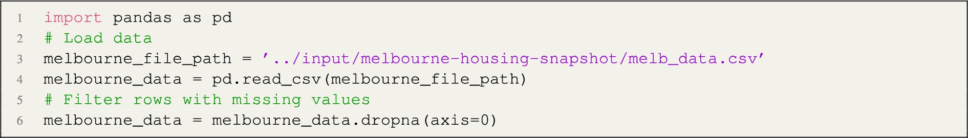 Line 1 and 3 mention references to resources: a software library (pandas) and a CSV file. The Kaggle notebook itself is the human readable and machine executable source code. When the python interpreter executes this script, it does so by the means of an intermediate machine representation, for example an abstract syntax tree is produced by parsing the code, and this is then exploited by the interpreter. However, the code structure implies knowledge that is not explicitly stated. This include the data flow, as defined in [17], which provides an abstraction of the way data is transferred and manipulated from the file in Line 3 to the variable melbourne_data in Line 6 (datanode graph). Finally, this source hides high-level intentions, for example, the fact that libraries and data are reused and some data preparation is performed, i.e., a column is dropped in Line 6 (activity graph).
While the first three components pre-exist the data journey, i.e. they do not pertain to the knowledge level [50], the remaining represent two distinct, although interconnected, representation layers. Here, we aim at automatically constructing such a layered representation, to demonstrate that data journeys can be automatically identified from the source code of a data science pipeline.
4.Ontology
We build on previous work and design an ontology as the reference knowledge model of a data journey, satisfying our definition. Our methodology is based on reusing successful, relevant models, completing them with concepts derived from the data used in this work. Specifically, we reuse concepts from three approaches: the W3C Provenance Ontology PROV-O [35], the Workflow Motifs Ontology [22] and the Datanode ontology [15]. Compared to the pre-existing models, DJO provides a unified view of the data journey, linking the two layers (the data flow layer and the activity layer). In addition, it extends the Datanode Ontology by specifying node types.
The Data Journey Ontology (DJO) reuses fundamental concepts from those three ontologies into a new conceptual model with layered semantics. The namespace of the DJO is http://purl.org/datajourneys/, the preferred prefix is djo. The design rationale of DJO is one of layered semantics. The ontology should be able to capture fine-grained data flows but also high-level activities, as super-imposed abstractions. An overview of the ontology is provided in Figs 1 and 2.22 We note that we align with broader software engineering concepts rather than specific machine learning notions as the aim here is to represent a generic data processing pipeline.
Fig. 1.
DJO: overview of the classes.
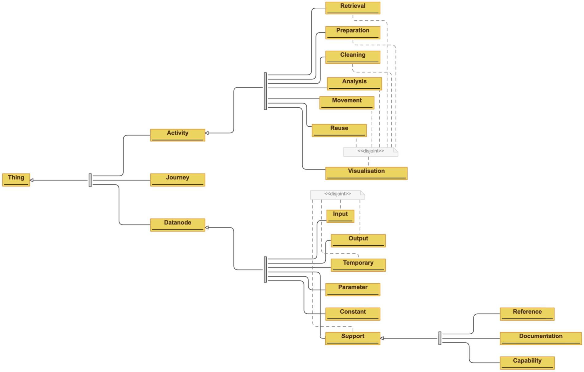
The core components are three classes: Datanode, Activity, and Journey.
Datanode The Datanode class represents a data object. We performed a thematic analysis of 20 randomly chosen notebooks from the dataset collected for the experiments (more about it in Section 6) in order to identify possible data node types, depending on the role they have in the process.
The result is as follows:
– Constant: a value hard-coded in the source code, for example, the value of an argument of a machine learning instruction
– Input: a pre-existing data object served to the program for consumption and manipulation.
– Output: a data node produced by the program
– Parameter: any data node which is not supposed to be modified by the program but is needed to tune the behaviour of the process. For example, the process splits the data source into two parts, 20% for the test set and 80% for the training set. 2, 20%, and 80% are all parameters.
– Support: any data node pre-existing the program, which is used without manipulation. Includes:
∗ Reference: any datanode used as background knowledge by the program, for example, a lookup service or a knowledge graph. Such datanode pre-exists the program and is external to the program.
∗ Capability: any datanode which provides capabilities to the program, including pre-existing modules, functions, and imported libraries.
∗ Documentation: any datanode which does not affect the operation of the program, such as source code comments and documentation.
– Temporary: any datanode produced and then reused by the program that is not intended to be the final output
– Input, Output, Support, and Temporary
– Capability, Documentation, and Reference
Table 1
List of object properties connecting instances of class Datanode in the Data Journey Ontology. Sources: PROV-O (PO), Datanode Ontology (DN), and Workflow Motifs (WM)
| Property | PO | DN | WM |
| derivedFrom | ✓ | ✓ | |
| analysedFrom | ✓ | ✓ | |
| cleanedFrom | ✓ | ✓ | |
| computedFrom | ✓ | ||
| copiedFrom | ✓ | ||
| movedFrom | ✓ | ✓ | |
| optimizedFrom | ✓ | ||
| preparedFrom | ✓ | ||
| augmentedFrom | ✓ | ||
| combinedFrom | ✓ | ✓ | |
| extractedFrom | ✓ | ✓ | |
| filteredFrom | ✓ | ✓ | |
| formatTransformedFrom | ✓ | ||
| groupedFrom | ✓ | ||
| sortedFrom | |||
| splitFrom | |||
| refactoredFrom | ✓ | ||
| remodelledFrom | ✓ | ||
| retrievedFrom | ✓ | ||
| visualisedFrom | ✓ |
Fig. 2.
DJO: overview of the properties.
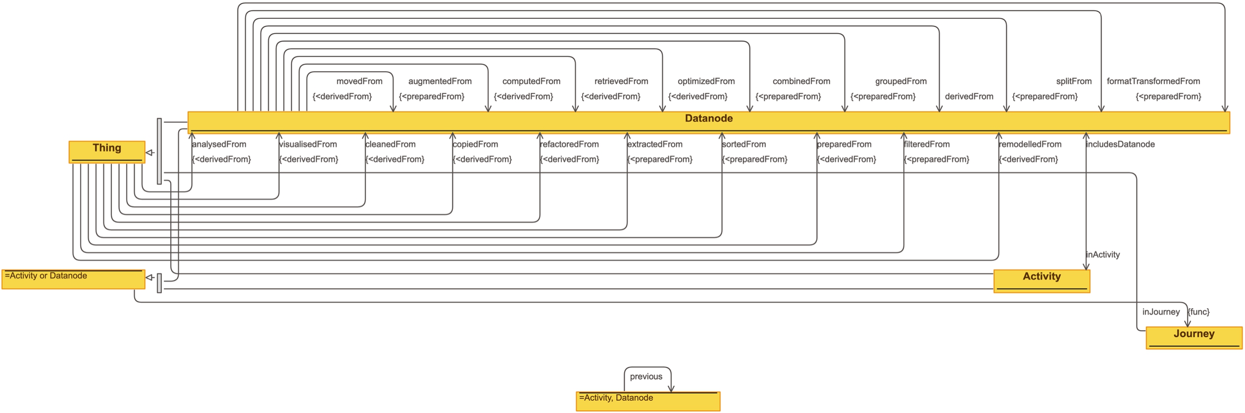
Activity In a Data Journey, sibling datanodes are supposed to be grouped together in activities, in order to provide a more abstract representation of the data journey. The activities included in DJO are mutually disjoint sub-classes of Activity: Analysis, Cleaning, Movement, Preparation, Retrieval, Reuse, and Visualisation. Except for Reuse, the other classes are derived from concepts defined by the Workflow Motifs ontology. Activities instances are connected to each other in a sequence, using the object property previous (and its inverse next. We note that the semantics of these two properties does not imply derivation but merely states the sequence of activities in a data journey. This approach in representing lists is inspired by the Sequence ontology design pattern33 [13,55] (see also [20] for a survey on modelling solutions for treating sequential information in RDF). Each activity instance is then connected to the involved datanodes through the property includesDatanode (and its inverse inActivity).
Journey Finally, both activities and Datanodes are meant to be connected to one data journey via the functional property inJourney.
Table 2 illustrates how DJO relates to fundamental concepts of data mining and machine learning workflows, as defined by two domain-specific ontologies for data mining (DMOP [33]) and machine learning (ML-Schema [56]). DJO can be extended by direct reuse of those concepts. In addition, DJO covers a broader set of notions familiar to any data science experiment, including, for example, visualisation and reuse.
Table 2
Conceptual mappings between DJO, DMOP and ML-schema
| DJO | DMOP | ML-Schema |
| Journey | DM-Workflow, DM-Process, DM-Experiment | Study, Experiment, Run |
| Datanode | ||
| Datanode > Constant | HyperParameterSetting | |
| Datanode > Input | IO-Object, DM-Data | Data, Dataset |
| Datanode > Output | IO-Object, DM-PatternSet, DM-Model | Model, ModelEvaluation |
| Datanode > Parameter | Parameter | HyperParameter |
| Datanode > Temporary | Dataset, Feature | |
| Datanode > Support | ||
| Datanode > Support > Reference | Measure | Data, Dataset, EvaluationMeasure, EvaluationSpecification, EvaluationProcedure |
| Datanode > Support > Capability | DM-Software, DM-Operator, DM-Model | Model, Feature, Software, Implementation |
| Datanode > Support > Documentation | DM-Task, DM-Algorithm, DM-Hypothesis, DM-Operation | Task, Algorithm, ModelCharacteristic, DataCharacteristic, ImplementationCharacteristic |
| Activity | DataProcessingTask | |
| Activity > Analysis | InductionTask, ModelingTask, PatternDiscoveryTask | |
| Activity > Cleaning | DataCleaningTask | |
| Activity > Movement | ||
| Activity > Preparation | DataReductionTask, DataAbstractionTask, DataTransformationTask | |
| Activity > Retrieval | ||
| Activity > Reuse | ||
| Activity > Visualisation |
5.Extracting data journeys
In this section, we describe our approach to extracting data journeys. An application of the method with a step-by-step example will follow in Section 6. Specifically, we examine the problem of automatically deriving data journeys from source code, focusing on identifying activities and their composition. We ground our method on the following hypothesis:
Given a data science program, it is possible to automatically extract a data journey from the code (a) by generating a datanode graph from the code; (b) making use of machine learning techniques to classify high-level activities in such graphs automatically; and (c) collapsing adjacent activity nodes involved in the same activity.
The method assumes source code as input (e.g. a python notebook), then generates a data node graph reusing symbols from the code (variable names, functions, operators, etc...). It then uses this information to train a classifier for identifying activity types. We note that we only focus on the generation of the data node graph structure and on the activity types, leaving the automatic support for the remaining features of the ontology (e.g. data node arc labelling and node types) to future work.
We divide the approach into four steps: (i) data node graph extraction, (ii) knowledge expansion, and (iii) knowledge compression.
In the first step – data node graph extraction – the method traverses the code Abstract Syntax Tree (AST) and transforms the structure into a Datanode graph. In such a graph, nodes represent data elements (such as files, variables, constants, and libraries), while arcs represent relationships, labelled with operations derived from the code – e.g. importing a library or assigning a variable – or with names of functions, method calls, or operators.
In the second step – knowledge expansion – we aggregate the data node graphs into a knowledge graph and derive frequent relationships (arcs in the graph) in a Frequent Activity Table (FAT). The most frequent activities are then annotated with the Data Journey Ontology (limited to Activity types in our experiments). The FAT allows us: (a) to generate automatically a set of rules encoded in SPARQL CONSTRUCT queries, to materialise the annotations, and (b) to produce a dataset of annotated data node graphs for training a classifier able to assign an Activity to each node in the data node graph. Furthermore, the classifier is applied to derive DJO activities automatically.
In the last step – data journey generation, adjacent nodes with the same activity types are collapsed, producing a summarised, compact, semantic representation of the data science pipeline – completing the Data Journey.
In the following sections, we describe each step in the abstract, leaving the details of the execution to the evaluation section, where we apply it to Python notebooks [53]. While we use Python here, the approach applies to any programming language that can be expressed as an AST.
5.1.Datanode graph extraction
We describe deriving a data node graph from a Python notebook. The algorithm implements heuristics, transforming the code structures into a graph. We organise the process in three steps:
Listing 1 illustrates the algorithm that generates the directed graph in pseudo-code.
Listing 1.
Pseudocode of the algorithm to extract a directed graph from the Python code
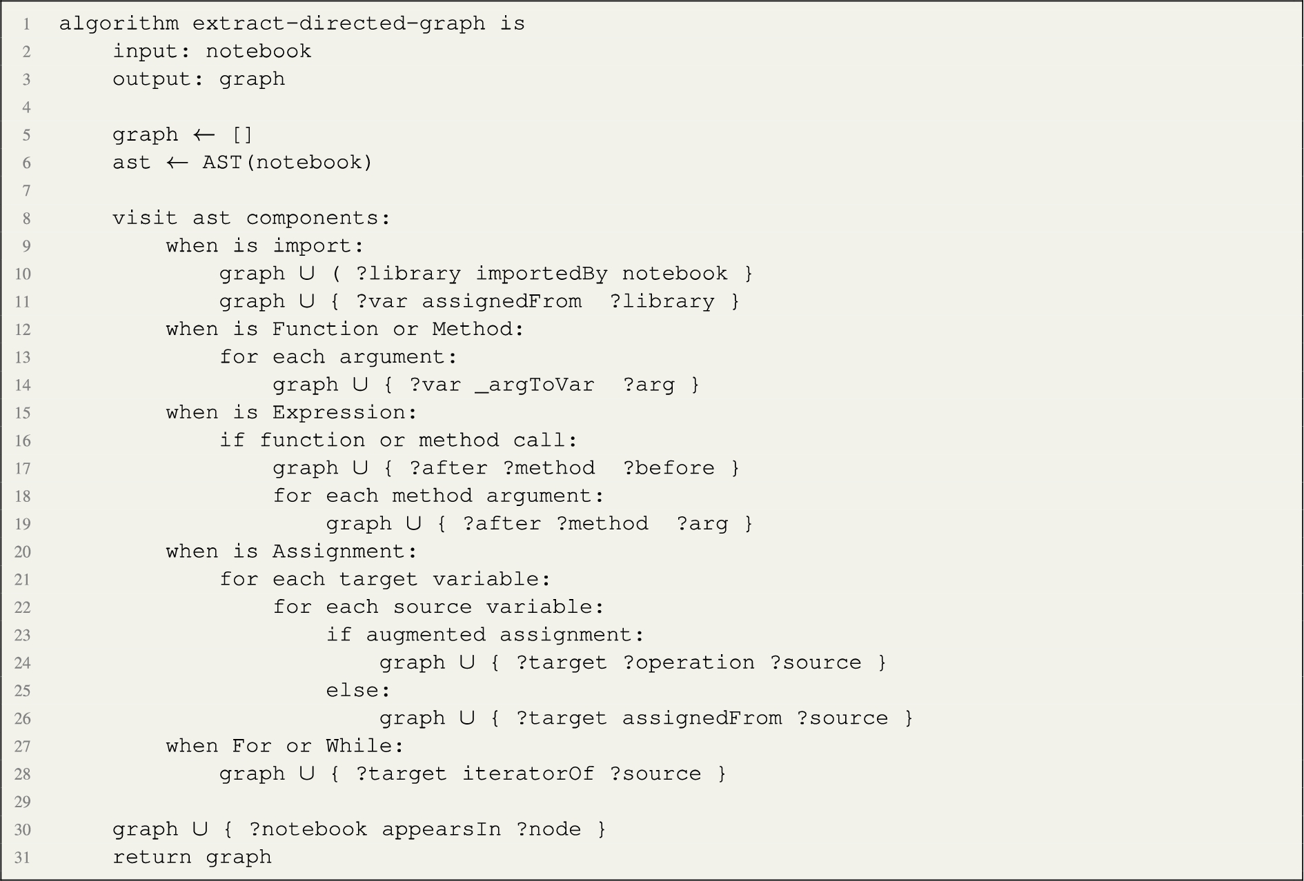
The process starts with traversing the Abstract Syntax Tree (AST) to build a directed graph where the nodes are data objects, such as libraries, files, constant values, and occurrences of variables, and arcs are dependency relationships, in the spirit of provenance models. The algorithm assigns unique identifiers (and human-readable labels) to graph nodes and assigns relationships applying an initial semantic layer derived from the code syntax (e.g. considering elements such as import, assignment operators, or function calls). The algorithm takes as input a python notebook and outputs an RDF graph. First, the graph is initialised (empty) and the abstract syntax tree derived by reusing a standard library. Then, AST components are traversed. Each one of the possible components of the Python programming languages are handled by dedicated heuristics. An import statement is interpreted as linking the notebook to the library, and the library to the variable that references it. Modules and Classes are not mapped directly in the data flow, while their components are inspected. Function and method definitions (line 12) are represented by linking the local variables to the function arguments (later calls to the function will link the input variables to the function arguments). Expressions are traversed by connecting variables and function or method arguments via the function or method names). Assignments are traversed by linking the variables accordingly. Finally, control operators such as if, when, etc. are not considered, apart from mapping variables accordingly, by flattening multiple iterations in a single data flow. Finally, all data nodes are mapped to the notebook with the appearsIn relation. The output of this step is a directed graph where nodes are data objects and arcs are relationship types derived from the code syntax.
The resulting directed graph is re-engineered into RDF. The direction of the arcs is reversed in the spirit of provenance graphs. In addition, we generate links from the notebook entity to each of the variable nodes. Furthermore, we add namespaces and use an entity function, which returns an RDF resource from the node label, applying the appropriate conversions to valid URI strings. The result is a data node graph, the first layer of our Data Journey.
5.2.Knowledge expansion
The previous section described obtaining a data node representation from the source code. This section will use the data node graph to derive background knowledge for training a Machine Learning algorithm able to annotate nodes with data journeys activities. Background knowledge includes the following components:
– The Data Journeys Ontology (DJO), introduced in Section 4, which specifies the following activity types: Reuse, Movement, Preparation, Analysis, and Visualisation
– A dataset of (frequent) data node arcs, manually annotated with DJO Activities – Frequent Activity Table (FAT)
– A set of rules (encoded as SPARQL construct queries) mapping frequent arcs in the data node graphs to DJ Activities, using the FAT – Frequent Activity Rules (FAR)
– Training dataset for the machine learning model, to predict Activities of unknown data node nodes – Machine Learning Training Dataset (MLTD)
Frequent Activity Table (FAT) From a statistical analysis of the data node graphs, the frequent arcs types can be determined. Such arcs are manually annotated with activity types. For example, nodes receiving an arc named “dj:importedBy” can be associated to a Reuse activity, or an arc derived from a popular function such as read_csv to a Movement activity. Similarly, a print arc demonstrates a Visualisation activity, and so forth. The objective is to have sufficient coverage of activity types in the table to use the annotation for training a machine learning model able to automate such annotations on all nodes in the data node graphs.
Frequent Activity Rules (FAR) From the FAT, we build rules to materialise the annotations. These are encoded as SPARQL CONSTRUCT queries to apply to the dataset of data node graphs.
Machine Learning Training Dataset (MLTD) We derive a training dataset from the table of annotated data node arcs. The input data includes a set of data nodes annotated with activity types (derived from the FAT). We can then enhance the activity types with background knowledge from existing knowledge models such as CodeBERTa [29] or produce RDF2Vec [58] embeddings directly from the data node graphs.
Machine learning application We use the dataset to evaluate the performance of potential ML approaches. Specifically, we evaluate a set of machine learning methods to automatically annotate the missing nodes with activity types in this phase. The most promising method is selected and applied to predict the activities of remaining and less frequent nodes.
5.3.Knowledge compression
We annotated the data node graph with activity types in the knowledge expansion phase. In this phase, we aim at obtaining a summarised view of the data journey. The knowledge compression task has the objective of generating activity instances by analysing sibling data nodes annotated with the same activity type. Activities may span multiple adjacent data nodes. For example, a Reuse activity applies to all imported libraries. Therefore, a better representation would generate a single instance of Reuse’s activity type, grouping all the import data nodes under a shared activity instance. The output is an Activity graph, whose nodes are instances of activities and arcs the previous relation. Crucially, activities may occur multiple times in different parts of the data node graph.
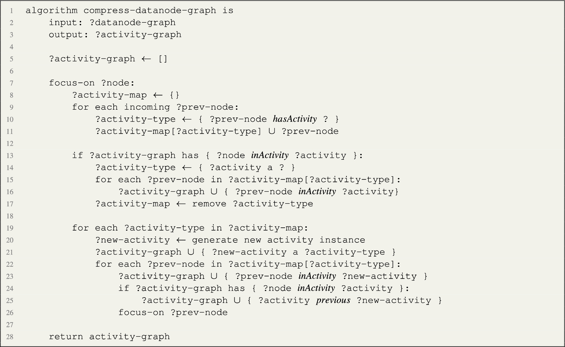
The process starts from the root of the data node graph (the nodes that don’t have outgoing arcs). Nodes are inspected for their annotated activity type. Every time a new activity type is found in the path, a new node is created of type Activity. If the node is annotated with the same activity type in the path, the existing activity node is mapped to the data node. The algorithm, illustrated in Listing 2, implements the following recursive pipeline, starting from the root node (the program):
1. Focus on a node and collect the set of previous nodes. Then, group those nodes by activity type, relying on the annotation property hasActivity, produced in the previous phase.
2. If the focus node was already linked to an activity instance in a previous iteration (property inActivity), link previous nodes having the same activity type to that activity instance with an inActivity property.
3. Generate a new activity instance for each remaining group, linking the related nodes with an inActivity relation.
4. Link the new activity instances to the focus node activity instance with a previous relation
5. Repeat for each previous node
Listing 2.
Pseudocode of the algorithm to compress the datanode graph and generate an activity graph.
6.Evaluation
To support XAI via exploration, we want to extract compact abstract representations of the data science workflows that are used to build AI systems (i.e. data journeys). These representations should provide a more accessible overview of these systems by virtue of being both smaller and by being tied to higher level concepts (e.g. Visualisation).
Hence, this section evaluates our hypothesis that it is possible to automatically derive a data journey by applying a combination of methods that abstract the source code into a layered, semantic representation. Specifically, we perform experiments to evaluate the effectiveness of classifying nodes within the program with higher-level semantics as expressed in the Data Journeys Ontology. Crucially, we aim to verify whether the graph structure is helpful in this classification process over just the use of the code itself. We evaluate:
1. the feasibility of automatically generating a graph representation, anchored to the source code,
2. the ability of data node graphs to support the automatic classification of activity types, and
3. the ability of activity graphs to offer a representation that is substantially more compact than the data node graph.
In the remainder of the section, we follow the approach introduced in Section 5, and we apply it to Python notebooks. Our dataset consists of the 1000 most popular python55 notebooks from Kaggle66 as of April 2020. Kaggle is one of the main hosts for data science competitions. Data node graphs are constructed for each notebook.
The implementation of the approach and all data assets used in the evaluation are provided for auditing and reproducibility [19].
6.1.Datanode graph extraction
In this step, we apply the algorithm described by Listing 1, which generates the directed graph. For example, given the following python code snippet (Kaggle: https://www.kaggle.com/dansbecker/random-forests): 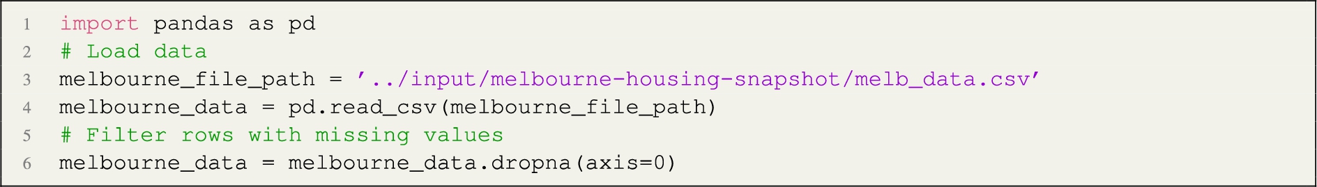 the algorithm generates the following directed graph, represented here in DOT format:
 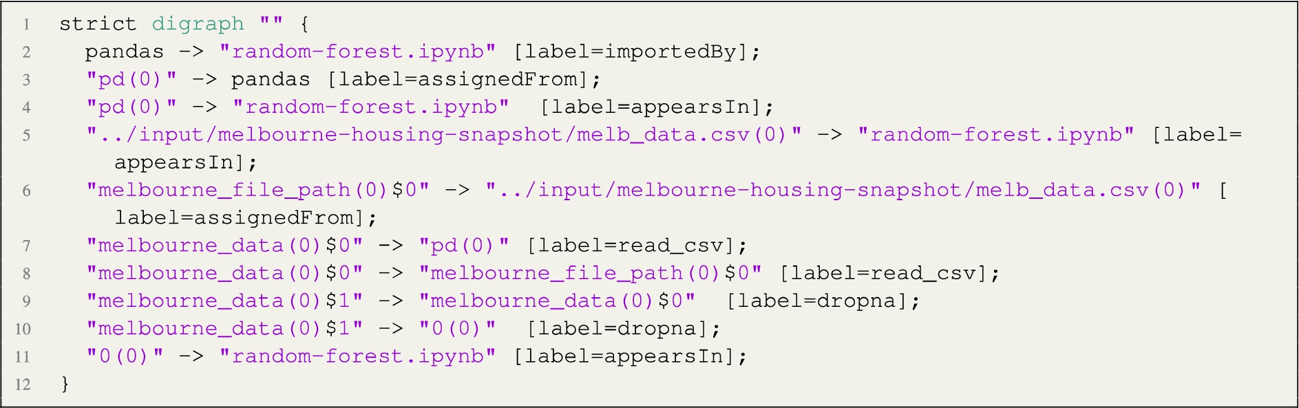 The arcs of the graph incorporate semantics derived from the code structure, partly assigned from heuristics in the algorithm, and partly derivable from the names of operators used in the code. For example, the relation importedBy links a library to the python script; the relation add links a variable (or constant) to its target variable; the relation print links a processing node to an output node; the relation assignedFrom is applied to local handlers of imported libraries as well as regular variable assignment operations. In addition, the example shows how the implementation takes care of linking multiple occurrences of the same variable together, generating a new node every time the variable value changes (for example, when re-assigned or when a method is called on a variable object, assuming the internal state of the data object is affected by the method call). Finally, the implementation ensures that variables are interpreted in the context of their scope. The number in parenthesis represents the outer scope, while the dollar sign distinguishes different instances of the same variable name. For example, it distinguishes a variable name used within the context of a function from the same variable name used in the outer scope (e.g. melbourne_data, lines 7–10).
The resulting directed graph is re-engineered into RDF. In particular, the direction of the arcs is reversed. Then, we add links from the notebook entity to each one of the nodes. In addition, we add namespaces and use an entity function which returns an RDF resource from the node label, applying the appropriate conversions to valid URI strings. In the implementation, we use the following namespaces: 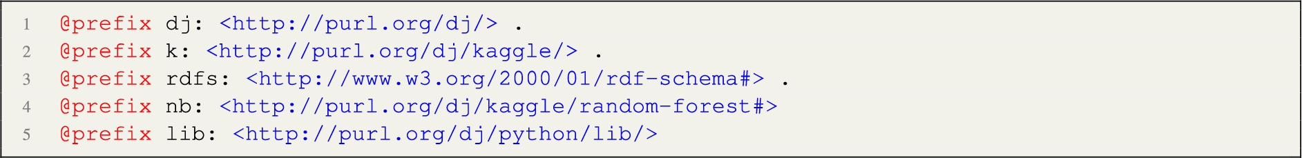 The k: namespace prefix is used for naming notebooks, the lib: namespace prefix is applied to python libraries, while the default namespace is used for any other entity generated. The above code generates the following data node graph in RDF:
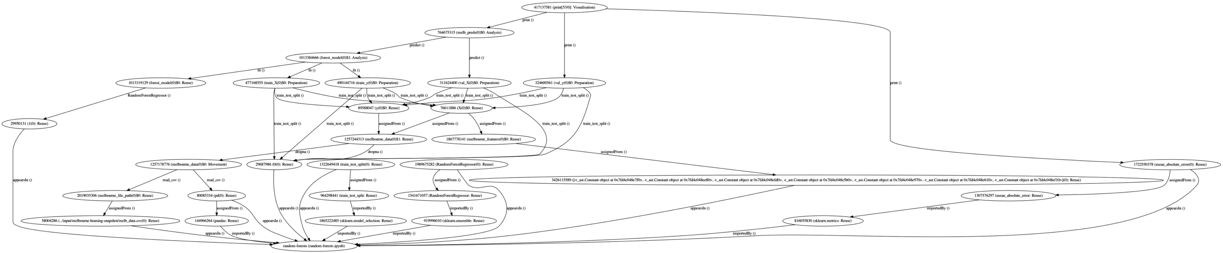
 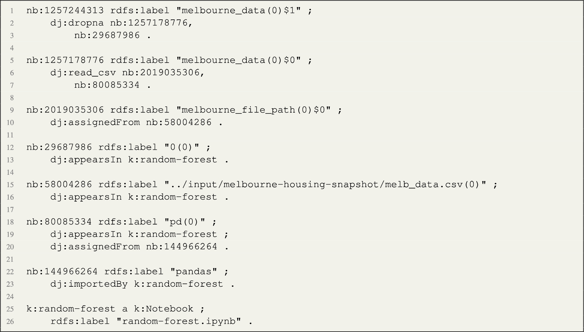 The execution of the process produces 804 data node graphs (we provide an example visualisation of one data node graph in Fig. 3. The remaining notebooks either included syntax errors, they did not include any source code, or the process took more than 10 minutes to complete. We leave the study of possible optimisations to future work.
Fig. 3.
Datanode graph of the random-forests data journey.
6.2.Knowledge expansion
The output of the previous phase are data node graphs expressed in RDF. Such a representation has the benefit that it is directly linked to the source code, to enable a graph representation to be overlayed on the program code. In this phase, we aim at identifying activities for each one of the node. Data node arcs are labelled according to clues derivable from the code (e.g. import statements and assignments, see Listing 1) or by reusing code elements (e.g. object methods, function names,…).
Frequent Activity Table (FAT) Following our method, we compute statistics of data node arcs and focus on the most frequent relationships in a Frequent Activity Table (FAT). The dataset includes 3384 distinct relations, from the more frequent ones (the most frequent being assignedFrom, 90370 occurrences) to relations occurring less frequently. We manually annotated the arcs occurring at least 2000 times in the dataset with data journey activities. The intended meaning is that when a given relation occurs, the target node can be qualified as being the result of the specified activity.77 Table 3 shows the relations occurring at least 1000 times in the dataset and related annotations. However, we observed that the Movement activity was underrepresented in the table; therefore, we selected two more arcs mapped to that activity.
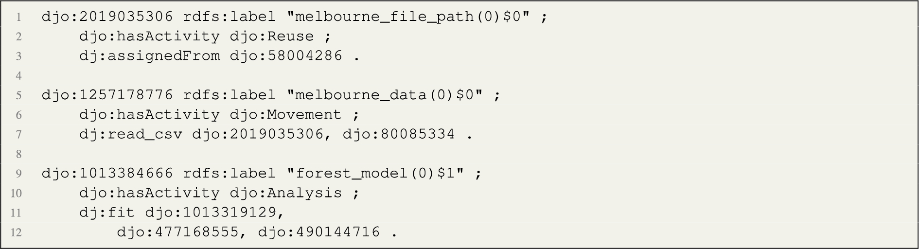
Frequent Activity Rules (FAR) From the FAT, rules are derived and encoded as SPARQL CONSTRUCT queries. Listings 3 and 4 show examples of such rules. The rules materialise a new statement using the DJO annotation property hasActivity, connecting data node entities to subclasses of Activity. We apply the rule sets to the data node graphs and materialise the new triples. An excerpt related to the guide example can be seen in Listing 5.
Table 3
Frequent Activity Table (FAT). Relations occurring at least 1000 times in the datanode dataset and related annotations. The table also distinguishes relations explicitly asserted by the AST traversal algorithm and the ones that are implicitly derived from the code
| Datanode arc | Occurrences | Asserted | Annotation |
| 16888 | :Visualisation | ||
| iteratorOf | 11825 | Y | :Preparation |
| importedBy | 10855 | Y | :Reuse |
| _argToVar | 9713 | Y | :Reuse |
| Add | 7334 | + | :Preparation |
| append | 6840 | :Preparation | |
| subplots | 6128 | :Visualisation | |
| apply | 5471 | :Preparation | |
| Div | 5115 | / | :Preparation |
| fit | 4415 | :Analysis | |
| read_csv | 4412 | :Movement | |
| astype | 4191 | :Preparation | |
| plot | 4036 | :Visualisation | |
| train_test_split | 3667 | :Preparation | |
| tanh | 3546 | :Analysis | |
| DataFrame | 3494 | :Preparation | |
| title | 3243 | :Preparation | |
| mean | 3200 | :Preparation | |
| add | 2843 | :Preparation | |
| subplot | 2545 | :Visualisation | |
| drop | 2527 | :Preparation | |
| predict | 2483 | :Analysis | |
| merge | 2404 | :Preparation | |
| map | 2345 | :Preparation | |
| head | 2314 | :Preparation | |
| [...] | |||
| to_csv | 1033 | :Movement | |
| [...] | |||
| copy | 678 | :Movement | |
Listing 3.
We can infer from the datanode arc importedBy that the target node relates to a Reuse activity.

Listing 4.
We can infer from the datanode arc print that the target node relates to a Visualisation activity.

Listing 5.
Example of data nodes annotated with activity types.
Machine Learning Training Dataset (MLTD) We create a training dataset from the table of annotated data node arcs. The input data includes a set of data nodes annotated with activity types (derived from the FAT). These can be enhanced with background knowledge, such as from existing knowledge models such as BERTcode [21] or producing RDF2Vec embeddings [58] from the data node graphs. Activities in the FAT are not equally represented. For example, Reuse, Preparation, and Visualisation have many more nodes than Analysis and Movement. Therefore, we select four arcs for each activity to give more balanced coverage to the training data. These are highlighted in Table 3. The resulting dataset includes the following information: the notebook, the graph node, the arc used to derive the annotation, and the annotated activity. The data includes 802 notebooks and 29282 nodes. Statistics of arcs, activities, and number of nodes in the training dataset are reported in Table 4.88
Table 4
ML Training Dataset, statistic of activity types and nodes
| Arc | Activity | Nodes |
| fit | :Analysis | 1316 |
| tanh | :Analysis | 299 |
| predict | :Analysis | 959 |
| read_csv | :Movement | 1727 |
| copy | :Movement | 431 |
| to_csv | :Movement | 490 |
| Add | :Preparation | 2078 |
| append | :Preparation | 2111 |
| iteratorOf | :Preparation | 4499 |
| importedBy | :Reuse | 1622 |
| _argToVar | :Reuse | 9709 |
| plot | :Visualisation | 1408 |
| subplots | :Visualisation | 1705 |
| :Visualisation | 6405 |
Machine learning application In this phase, we train an ML model to annotate the missing nodes with activity types automatically. In the next section, we will report on experiments with multiple machine learning algorithms. We select the most promising method and use it to predict the activities of remaining non-frequent nodes. The output of the learned classifier is a data node graph whose nodes are all annotated with activity types, using the DJO OWL annotation property :hasActivity.
6.3.ML classification experiments
We train classifiers that, given a node representing an Activity from a notebook, predict its high-level semantic type – one of Analysis, Movement, Preparation, Reuse, Visualisation. We tested standard classifiers available in scikit-learn, specifically Logistic Regression, Decision Trees, Gaussian Naive Bayes, Linear Support Vector Machine and a Multi-layer Perceptron.
We develop tests using two different methods for representing nodes as input to the classifiers:
1. CodeBERTa – In this setting, we embed the code string associated with a node using CodeBERTa [29] a pre-trained transformed based language model trained on a large corpus of the programs from the CodeSearchNet [31]. The corpus used contains roughly 6 million functions spanning six programming languages.
2. RDF2Vec – In this setting, we use RDF2Vec [58] to embed each node based on its structural position in a knowledge graph constructed from the RDF representation of the notebooks used during the experiment. RDF2Vec is set to use the following parameters: the node is represented based on its context, i.e. a continuous bag of words (CBOW). The context is determined by extracting paths in a random walk around the node. A maximum of 100 paths are extracted with a maximum depth of 10.
For each setting, we employ two testing regimes:
R1 Nodes are randomly split between training and testing sets.
R2 Nodes are randomly split between training and testing sets but the train and test sets do not share notebooks.
A 70/30 train test split is used. Hyperparameters are as detailed above. R1 simulates the behaviour where one wants to classify other (e.g. long-tail) nodes from within a codebase, which contains some already classified nodes. Whereas R2 aims to simulate an environment in which one is trying to classify nodes from a notebook that has not been seen before. For each classifier, setting and regime combination, we use 10, 100 and 200 notebooks randomly sampled from the corpus. Experiments are repeated 10 times for each combination. Table 5 shows the average knowledge graph size across experimental runs.
The experiments showed an increasing accuracy when providing a larger set of notebooks. Table 6 presents the best results achieved when training with 200 notebooks. We report on two metrics: Accuracy and Matthews correlation coefficient.99 The best results are achieved by the Multi-Layered Perceptron classifier using the RDF2Vec embeddings method. With these results, we demonstrate that using a data node graph as an intermediate representation of the program improves the prediction accuracy systematically across all machine learning algorithms.
Table 5
The size of knowledge graphs per number of notebooks used across experiments
| Notebook count | Average KG size (nodes) |
| 10 | 8885 |
| 100 | 89202 |
| 200 | 186457 |
Table 6
Results for test regime R1 for multiple classifiers using a KG based on 200 notebooks
| Method | Accuracy | Matthews | ||
| mean | std | mean | std | |
| CodeBERTa | ||||
| Decision Tree | 0.49 | 0.36 | 0.32 | 0.48 |
| GaussianNB | 0.66 | 0.25 | 0.61 | 0.25 |
| LinearSVC | 0.43 | 0.45 | 0.25 | 0.58 |
| LogisticRegression | 0.05 | 0.00 | 0.00 | 0.00 |
| MLPClassifier | 0.40 | 0.40 | 0.30 | 0.45 |
| RandomForestClassifier | 0.52 | 0.31 | 0.33 | 0.45 |
| RDF2Vec | ||||
| Decision Tree | 0.68 | 0.06 | 0.58 | 0.07 |
| GaussianNB | 0.84 | 0.02 | 0.79 | 0.02 |
| LinearSVC | 0.95 | 0.01 | 0.93 | 0.02 |
| LogisticRegression | 0.95 | 0.01 | 0.93 | 0.02 |
| MLPClassifier | 0.96 | 0.01 | 0.95 | 0.01 |
| RandomForestClassifier | 0.85 | 0.01 | 0.80 | 0.02 |
6.4.Knowledge compression
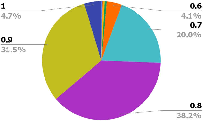
The output of the machine learning application phase is a datanode graph whose nodes are all annotated with activity types. However, such representation does not allow us to see the intended activities at a higher level of abstraction. In this final phase, we apply the algorithm described in Listing 2 to the notebooks from the prior stage in order to generate a summarised view of the program by creating instances of activities in our ontology, absorbing adjacent data nodes annotated with the same activity type. Here, we evaluate the ability of the approach to generate a more abstract representation of the process, by reducing the number of nodes required to express the data science pipeline. Specifically, we compare the size (number of arcs) of the data node layer with the one of the activity layer of the data journeys produced. Figures 4 displays the distribution of this compression factor, computed as the ratio between the number of arcs of the data node graph and the ones of the activity graphs. The numbers demonstrate that our approach provides an effective way of summarising the data science pipelines, with almost all of the activity graphs being more than half of the size of the respective data node ones. Crucially, there has been a reduction of at least 0.8 factor in about 3/4 of the cases.
Fig. 4.
Compression factor – the percentage of the notebook corpus that were compressed by the indicated amount.
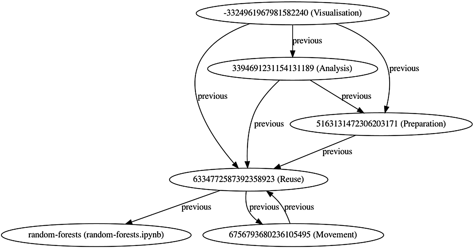
Following the example introduced at the beginning of this section, the random-forests data journey contains 84 entities in the data node layer and only 18 in the activity graph layer, for a compression factor of .78. Figure 5 shows the activity graph (the equivalent data node graph is in Fig. 3). The first representation accurately describes the data flow, but it is also very difficult to explore. The second, is a much more compact representation of core activities. Crucially, our layered approach allows us to use the more synthetic representation as a proxy to the underlying one and, indirectly, to the actual source code.
Fig. 5.
Activity graph of the random-forests data journey.
7.Exploratory user survey
We performed an exploratory user survey to evaluate the validity of our proposal and its potential interest to data science practitioners.
7.1.Participants
To that end, we performed convenience sampling and disseminated a questionnaire to researchers and data technologists known to the authors and collected twelve responses. Participants agreed on sharing anonymous survey results in publications.
Our survey participants are all data science technologists. While sharing a high technical expertise, their experience span a variety of support systems and are, therefore, a good representative of our target user base.
Four participants have more than five years of practical experience in data science, seven of the participants have between one and five years of experience, while one of them has less than one year.
When asked to self-assess their confidence with data science methods and/or tools on a Likert scale of 1 (not at all) to 5 (very confident), the majority of the participants indicated 4 (10), while the remaining two participants replied 3 (medium) and 2 (low), respectively.
When asked about how much they rely on user-friendly support tools rather than writing code directly, on a Likert scale of 1 (code directly) to 5 (tool support), there was a clear preference to writing code, with only one participant replying 4 and none of them 5. Interestingly, only 25% of the participants use debugging or troubleshooting support tools as part of their development process. When asked, they mentioned the Pycharm debugger,1010 Kedro,1111 Visual Studio,1212 and Papermill.1313 Most of the survey participants use data science notebooks and mentioned environments such as Jupyter,1414 Databricks,1515 RStudio,1616 or Google Colaboratory1717 (11 out of 12).
7.2.Feedback on DJO
With the objective of assessing the coverage of DJO, we asked participant whether they recognised the activities of the ontology in their own practice, on a Likert scale of 1 (never) to 5 (always). Results are presented in Fig. 6.
Fig. 6.
Answers to the question: “do you recognise these high level steps in your data science process?”
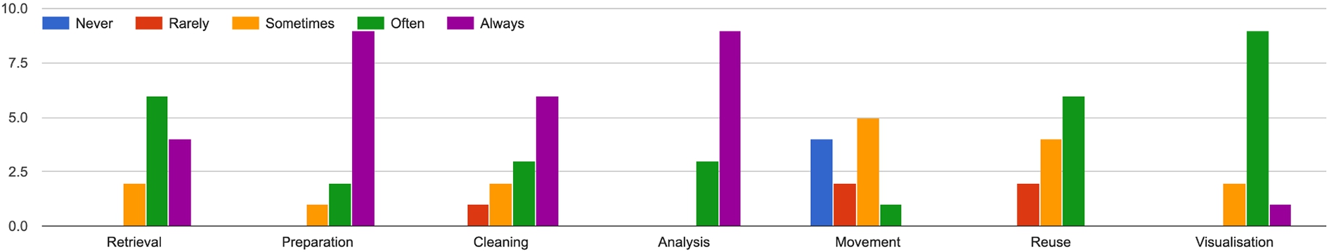
We asked participants if they could think of any step missing, and received two types of answers. The first relates to activities such as exploration, modelling, publishing, dissemination, testing, monitoring and maintenance, and deployment. These are all relevant activities, typically conducted during the design and development phases. However, they are describing activities of developers rather than activities of the data science pipeline. The second relates to machine learning-specific operations such as training, prediction, and validation. In our work, we avoided including ML-specific terminology with the purpose of generality, and consider those activities a special type of Analysis. However, DJO could be extended and specialised to support ML-specific activities, for example, reusing notions from Onto-DM [52].
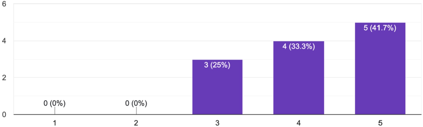
With the purpose of assessing the sufficiency of DJO, we asked participants to judge the appropriateness of the classes proposed, from the point of view of their level of abstraction, on a Likert scale of 1 (too much detailed) to 5 (too much abstract). Eight participants out of twelve replied with option 3, while the remaining four judged them possibly abstract (option 4) but never too much (option 5).
Next, we moved on evaluating the types of objects considered by DJO (see Fig. 1) We asked participants if they recognised those high level types of object in their data science process. The answers are summarised in Fig. 7 Crucially, the majority of the responses lean towards considering the DJO object types necessary for capturing the meaning of data science pipelines. When asked if they could think about missing object types, some of them provided feedback pointing to further roles that can be given to data objects, for example, specialising DJO type reference into baseline and control, and considering metric as a sub class of capability.
Furthermore, we asked survey participants to provide feedback on the data-to-data operations (relations) that could link data objects in the datanode layer of DJO (see Table 1 and Fig. 2). Feedback shows how all the relations included in DJO play a substantial role for data science practitioners, with only a few responses leaning towards rarely or never used (the least “popular” relations being remodelling, refactoring, and augmenting; see Fig. 8). Instead, when asked for feedback about potentially missing relations, we had very few suggestions, mainly referring to notions already emerged previously, such as predicting, classifying, reporting, disseminating, and packaging. Some of those are possible specialisations of existing relations, e.g. predicting and classifying are special cases of analysing. Instead, reporting and disseminating are not relations between data objects, while packaging can be considered a special case of format transforming. Ultimately, this feedback reassure us on the sufficiency of the ontology to cover the generality of data science workflows.
Fig. 7.
Answers to the question: “do you recognise these high level object types in your data science process?”
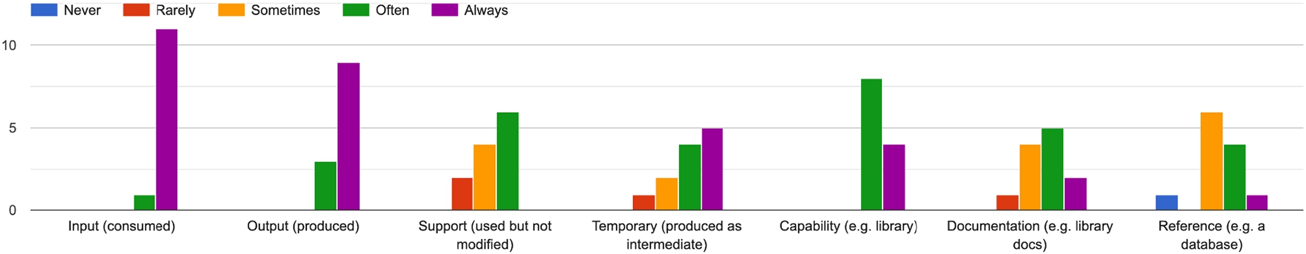
Fig. 8.
Answers to the question: “do you recognise these operations on objects of your data science pipelines?”

7.3.Feedback on concrete data journeys
In the last part of the survey, we presented three examples of data journeys, and we asked few questions about this type of data science pipeline representation.
Specifically, we asked participants to review data journeys generated from three Kaggle notebooks, selected for being representative of three families of data science activities:
Fig. 9.
Answers to the question: “in what task would you see the representation helping?”
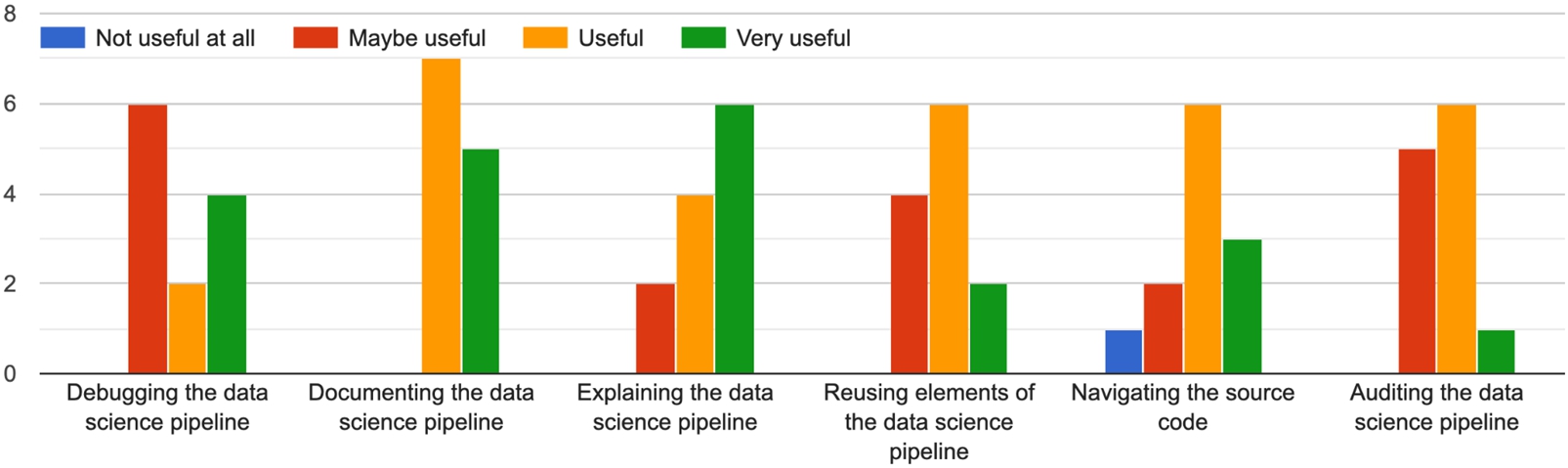
Feedback shows how data journeys are perceived as useful for all these tasks, and especially useful for explaining data science workflows (we received the highest positive feedback on this task, specifically). When asked if data journeys could be useful to other tasks, users mentioned pipeline information retrieval, pipeline pattern recognition, pipeline handover/onboarding, as well as education and visualisation. Additionally, survey participants comments included the need of developing tools and particularly UIs to support data journeys (to hide the technical underlying representation of the pipeline and make it more readable). Data journeys could be used for navigating the source code, and using the representations as presented in this survey (graph-like diagrams) directly may be a bit difficult.
We concluded the survey asking for a general assessment about the utility and value-to-users of data journeys, which is shown in Fig. 10. Overall, this preliminary survey shows the benefit of Data Journey style representations for tasks related to the explanation of how AI systems are constructed and trained.
Fig. 10.
Answers to the question: “would you like to have a data journey alongside the source code?”
8.Conclusion
In this article, we proposed an ontology for representing Data Journeys and mechanisms for extracting them from data science notebooks in order to provide a basis for traced-based XAI. Using a corpus obtained from the 1000 most popular python notebooks on Kaggle, we showed how data journeys can be automatically identified from source code. The abstract representations that are generated are in many cases 80% the size of the original graphs. Additionally, our experiments show that an intermediate (datanode) graph representation (via RDF2Vec) improves performance over the use of just the code itself (via CodeBERTa) on the task of identifying high-level datascience activity.
There are several limitations to our current approach. First, the current implementation is limited to Python code, although the approach is portable to other languages. In addition, the implementation can be improved as there were notebooks could not be properly processed. Here, we focused on the Activity Graph layer of the data journey. We plan to expand our approach to include also the other components of the Data Journey ontology, specifically, by decorating the datanode layer with the richer types and relations specified in the Data Journey Ontology.
Importantly, data journeys provide an exciting foundation for further work in XAI. For example, exploring better debugging of machine learning pipelines through user interfaces and end user tools that take advantage of the overview that data journeys provide. There is also potential in incorporating more layers (e.g policies, specialised data science ontologies, or domain specific data view) that provide different ways of exploring AI system workflows.
Beyond XAI, data journeys can potentially provide a mechanism for compliance checking in terms of correct licensing, data privacy and attribution. In terms of open science, data journeys could provide the possibility to wire in expertise and explanation at different levels of abstraction.
We see a potential future in which data journeys with multiple layers of information about tasks, data, expertise, bias, can be used to build rich environments for transparency and explanation.
Notes
2 The visual representations are generated with OWLGrEd [39]: http://owlgred.lumii.lv/online_visualization.
3 Sequence ODP: http://ontologydesignpatterns.org/wiki/Submissions:Sequence.
5 As measured by the ‘hotness’ parameter of the API.
7 We note that the training data was annotated with only one activity, although several of those arcs may be classified under more that one activity. The activity is assigned based on the annotators knowledge of the corpus.
8 The data in the table was produced by querying the training dataset (CSV) using SPARQL Anything [7].
10 https://www.jetbrains.com/pycharm/ (Accessed 03/03/2023).
11 https://kedro.org/ (Accessed 03/03/2023).
12 https://visualstudio.microsoft.com/ (Accessed 03/03/2023).
13 https://papermill.readthedocs.io/en/latest/ (Accessed 03/03/2023).
14 https://jupyter.org/ (Accessed 03/03/2023).
15 https://azure.microsoft.com/en-us/products/databricks (Accessed 03/03/2023).
16 https://posit.co/products/open-source/rstudio/ (Accessed 03/03/2023).
17 https://colab.research.google.com/ (Accessed 03/03/2023).
18 The Kaggle notebook is https://www.kaggle.com/code/dansbecker/random-forests (accessed, 7/03/2023). The DJO representation of the data science pipeline can be found at this URL: https://github.com/enridaga/data-journeys/blob/master/datajourneys/random-forests.ttl.
19 https://www.kaggle.com/code/ngyptr/python-nltk-sentiment-analysis/notebook (accessed, 7/03/2023). The DJO representation of the data science pipeline can be found at this URL: https://github.com/enridaga/data-journeys/blob/master/datajourneys/python-nltk-sentiment-analysis.ttl.
20 https://www.kaggle.com/code/dimarudov/data-analysis-using-sql (accessed, 7/03/2023). The DJO representation of the data science pipeline can be found at this URL: https://github.com/enridaga/data-journeys/blob/master/datajourneys/data-analysis-using-sql.ttl.
Acknowledgements
This work was partially supported by the EU’s Horizon Europe research and innovation programme within the ENEXA project (grant Agreement no. 101070305), the SPICE project (Grant Agreement N. 870811), and the Polifonia project (grant angreemnt N. 101004746).
References
[1] | I. Abdelaziz, J. Dolby, J. McCusker and K. Srinivas, A toolkit for generating code knowledge graphs, in: Proceedings of the 11th on Knowledge Capture Conference, K-CAP’21, Association for Computing Machinery, New York, NY, USA, (2021) , pp. 137–144. ISBN 9781450384575. doi:10.1145/3460210.3493578. |
[2] | I. Abdelaziz, K. Srinivas, J. Dolby and J.P. McCusker, A demonstration of CodeBreaker: A machine interpretable knowledge graph for code, in: ISWC (Demos/Industry), 2020. |
[3] | ACM US Public Policy Council, Statement on algorithmic transparency and accountability, 2017. |
[4] | W. Ahmad, S. Chakraborty, B. Ray and K.-W. Chang, A transformer-based approach for source code summarization, in: Proceedings of the 58th Annual Meeting of the Association for Computational Linguistics, Association for Computational Linguistics, Online, (2020) , pp. 4998–5007, https://aclanthology.org/2020.acl-main.449. doi:10.18653/v1/2020.acl-main.449. |
[5] | S. Al Manir, J. Niestroy, M.A. Levinson and T. Clark, Evidence graphs: Supporting transparent and FAIR computation, with defeasible reasoning on data, methods, and results, in: Provenance and Annotation of Data and Processes, Springer, (2020) , pp. 39–50. |
[6] | A.I. Anik and A. Bunt, Data-centric explanations: Explaining training data of machine learning systems to promote transparency, in: Proceedings of the 2021 CHI Conference on Human Factors in Computing Systems, CHI’21, Association for Computing Machinery, New York, NY, USA, (2021) . ISBN 9781450380966. doi:10.1145/3411764.3445736. |
[7] | L. Asprino, E. Daga, A. Gangemi and P. Mulholland, Knowledge graph construction with a façade: A unified method to access heterogeneous data sources on the Web, ACM Transactions on Internet Technology (2022). |
[8] | M. Atzeni and M. Atzori, CodeOntology: RDF-ization of source code, in: International Semantic Web Conference, Springer, (2017) , pp. 20–28. |
[9] | A. Barredo Arrieta, N. Díaz-Rodríguez, J. Del Ser, A. Bennetot, S. Tabik, A. Barbado, S. Garcia, S. Gil-Lopez, D. Molina, R. Benjamins, R. Chatila and F. Herrera, Explainable Artificial Intelligence (XAI): Concepts, taxonomies, opportunities and challenges toward responsible AI, Information Fusion 58: ((2020) ), 82–115, https://www.sciencedirect.com/science/article/pii/S1566253519308103. doi:10.1016/j.inffus.2019.12.012. |
[10] | K. Belhajjame, J. Zhao, D. Garijo, M. Gamble, K. Hettne, R. Palma, E. Mina, O. Corcho, J.M. Gómez-Pérez, S. Bechhofer et al., Using a suite of ontologies for preserving workflow-centric research objects, Journal of Web Semantics 32: ((2015) ), 16–42. doi:10.1016/j.websem.2015.01.003. |
[11] | K. Cao and J. Fairbanks, Unsupervised construction of knowledge graphs from text and code, 2019, arXiv preprint arXiv:1908.09354. |
[12] | S. Chari, D.M. Gruen, O. Seneviratne and D.L. McGuinness, Directions for explainable knowledge-enabled systems, in: Knowledge Graphs for EXplainable Artificial Intelligence: Foundations, Applications and Challenges, IOS Press, (2020) , pp. 245–261. |
[13] | E. Daga, E. Blomqvist, A. Gangemi, E. Montiel, N. Nikitina, V. Presutti and B. Villazón-Terrazas, D2.5.2 Pattern Based Ontology Design: Methodology and Software Support, (2008) . |
[14] | E. Daga, M. d’Aquin, A. Adamou and E. Motta, Addressing exploitability of smart city data, in: 2016 IEEE International Smart Cities Conference (ISC2), IEEE, (2016) , pp. 1–6. |
[15] | E. Daga, M. d’Aquin, A. Gangemi and E. Motta, Describing semantic web applications through relations between data nodes, Technical Report kmi-14–05, Knowledge Media Institute, The Open University, Walton Hall, Milton Keynes, 2014. |
[16] | E. Daga, M. d’Aquin, A. Gangemi and E. Motta, Propagation of policies in rich data flows, in: Proceedings of the 8th International Conference on Knowledge Capture, (2015) , pp. 1–8. |
[17] | E. Daga, M. d’Aquin and E. Motta, Propagating data policies: A user study, in: Proceedings of the Knowledge Capture Conference, (2017) , pp. 1–8. |
[18] | E. Daga, A. Gangemi and E. Motta, Reasoning with data flows and policy propagation rules, Semantic Web 9: (2) ((2018) ), 163–183. doi:10.3233/SW-170266. |
[19] | E. Daga and P. Groth, enridaga/data-journeys: v1, 2021. doi:10.5281/zenodo.5770310. |
[20] | E. Daga, A. Meroño-Peñuela and E. Motta, Sequential linked data: The state of affairs, Semantic Web (2021), 1–36. |
[21] | Z. Feng, D. Guo, D. Tang, N. Duan, X. Feng, M. Gong, L. Shou, B. Qin, T. Liu, D. Jiang and M. Zhou, CodeBERT: A pre-trained model for programming and natural languages, in: Findings of the Association for Computational Linguistics: EMNLP 2020, Association for Computational Linguistics, Online, (2020) , pp. 1536–1547, https://aclanthology.org/2020.findings-emnlp.139. doi:10.18653/v1/2020.findings-emnlp.139. |
[22] | D. Garijo, P. Alper, K. Belhajjame, O. Corcho, Y. Gil and C. Goble, Common motifs in scientific workflows: An empirical analysis, Future Generation Computer Systems 36: ((2014) ), 338–351. doi:10.1016/j.future.2013.09.018. |
[23] | S. Grafberger, P. Groth and S. Schelter, Towards data-centric what-if analysis for native machine learning pipelines, in: Proceedings of the Sixth Workshop on Data Management for End-To-End Machine Learning, DEEM’22, Association for Computing Machinery, New York, NY, USA, (2022) , https://stefan-grafberger.com/mlwhatif-deem.pdf. ISBN 9781450393751. doi:10.1145/3533028.3533303. |
[24] | S. Grafberger, P. Groth, J. Stoyanovich and S. Schelter, Data distribution debugging in machine learning pipelines, The VLDB Journal ((2022) ), https://stefan-grafberger.com/mlinspect-journal.pdf. doi:10.1007/s00778-021-00726-w. |
[25] | S. Grafberger, J. Stoyanovich and S. Schelter, Lightweight inspection of data preprocessing in native machine learning pipelines, in: 11th Conference on Innovative Data Systems Research, CIDR 2021, Virtual Event, Online Proceedings, January 11–15, 2021, www.cidrdb.org, (2021) , http://cidrdb.org/cidr2021/papers/cidr2021_paper27.pdf. |
[26] | M. Herschel, R. Diestelkämper and H.B. Lahmar, A survey on provenance: What for? What form? What from?, The VLDB Journal 26: (6) ((2017) ), 881–906. doi:10.1007/s00778-017-0486-1. |
[27] | K. Holstein, J. Wortman Vaughan, H. Daumé, M. Dudik and H. Wallach, Improving fairness in machine learning systems: What do industry practitioners need?, in: Proceedings of the 2019 CHI Conference on Human Factors in Computing Systems, CHI’19, Association for Computing Machinery, New York, NY, USA, (2019) , pp. 1–16. ISBN 9781450359702. doi:10.1145/3290605.3300830. |
[28] | A. Holzinger, C. Biemann, C.S. Pattichis and D.B. Kell, What do we need to build explainable AI systems for the medical domain? 2017, arXiv preprint arXiv:1712.09923. |
[29] | huggingface/CodeBERTa-small-v1 · Hugging Face, https://huggingface.co/huggingface/CodeBERTa-small-v1. |
[30] | M.R. Huq, P.M.G. Apers and A. Wombacher, ProvenanceCurious: A tool to infer data provenance from scripts, in: Proceedings of the 16th International Conference on Extending Database Technology, EDBT’13, Association for Computing Machinery, New York, NY, USA, (2013) , pp. 765–768. ISBN 9781450315975. doi:10.1145/2452376.2452475. |
[31] | H. Husain, H.-H. Wu, T. Gazit, M. Allamanis and M. Brockschmidt, CodeSearchNet challenge: Evaluating the state of semantic code search, 2019, http://arxiv.org/abs/1909.09436. |
[32] | A. Ignatiev, Towards trustable explainable AI, in: Proceedings of the Twenty-Ninth International Joint Conference on Artificial Intelligence, IJCAI-20, C. Bessiere, ed., International Joint Conferences on Artificial Intelligence Organization, (2020) , pp. 5154–5158, Early Career. doi:10.24963/ijcai.2020/726. |
[33] | C.M. Keet, A. Ławrynowicz, C. d’Amato, A. Kalousis, P. Nguyen, R. Palma, R. Stevens and M. Hilario, The data mining optimization ontology, Journal of web semantics 32: ((2015) ), 43–53. doi:10.1016/j.websem.2015.01.001. |
[34] | F.Z. Khan, S. Soiland-Reyes, R.O. Sinnott, A. Lonie, C. Goble and M.R. Crusoe, Sharing interoperable workflow provenance: A review of best practices and their practical application in CWLProv, GigaScience 8: (11) ((2019) ), giz095. doi:10.1093/gigascience/giz095. |
[35] | T. Lebo, S. Sahoo, D. McGuinness, K. Belhajjame, J. Cheney, D. Corsar, D. Garijo, S. Soiland-Reyes, S. Zednik and J. Zhao, Prov-o: The prov ontology, 2013. |
[36] | S. Leonelli, Learning from data journeys, in: Data Journeys in the Sciences, S. Leonelli and N. Tempini, eds, Springer International Publishing, Cham, (2020) , pp. 1–24. ISBN 978-3-030-37177-7. doi:10.1007/978-3-030-37177-7_1. |
[37] | S. Leonelli and N. Tempini (eds), Data Journeys in the Sciences, Springer International Publishing, Cham, (2020) , ISBN 9783030371760, 9783030371777. doi:10.1007/978-3-030-37177-7. |
[38] | X.-H. Li, C.C. Cao, Y. Shi, W. Bai, H. Gao, L. Qiu, C. Wang, Y. Gao, S. Zhang, X. Xue et al., A survey of data-driven and knowledge-aware explainable ai, IEEE Transactions on Knowledge and Data Engineering (2020). |
[39] | R. Liepinš, M. Grasmanis and U. Bojars, OWLGrEd ontology visualizer, in: Proceedings of the 2014 International Conference on Developers, Vol. 1268: , CEUR-WS.org, (2014) , pp. 37–42. |
[40] | Z.C. Lipton, The mythos of model interpretability, in: Machine Learning, the Concept of Interpretability Is Both Important and Slippery., Queue, Vol. 16: , (2018) , pp. 31–57. doi:10.1145/3236386.3241340. |
[41] | R. Lourenço, J. Freire and D. Shasha, Debugging machine learning pipelines, in: Proceedings of the 3rd International Workshop on Data Management for End-To-End Machine Learning, DEEM’19, Association for Computing Machinery, New York, NY, USA, (2019) . ISBN 9781450367974. doi:10.1145/3329486.3329489. |
[42] | S.M. Lundberg and S.-I. Lee, A unified approach to interpreting model predictions, in: Proceedings of the 31st International Conference on Neural Information Processing Systems, NIPS’17, Curran Associates Inc., Red Hook, NY, USA, (2017) , pp. 4768–4777. ISBN 9781510860964. |
[43] | S. Mohseni, N. Zarei and E.D. Ragan, A multidisciplinary survey and framework for design and evaluation of explainable AI systems, ACM Trans. Interact. Intell. Syst. 11(3–4) (2021). doi:10.1145/3387166. |
[44] | L. Moreau, The Foundations for Provenance on the Web, Now Publishers Inc, (2010) . |
[45] | L. Moreau and P. Groth, 2013, PROV-Overview, W3C Note, W3C, https://www.w3.org/TR/2013/NOTE-prov-overview-20130430/. |
[46] | L. Moreau, P. Groth, S. Miles, J. Vazquez-Salceda, J. Ibbotson, S. Jiang, S. Munroe, O. Rana, A. Schreiber, V. Tan et al., The provenance of electronic data, Communications of the ACM 51: (4) ((2008) ), 52–58. doi:10.1145/1330311.1330323. |
[47] | S.T. Mueller, R.R. Hoffman, W. Clancey, A. Emrey and G. Klein, Explanation in Human-AI Systems: A Literature Meta-Review, Synopsis of Key Ideas and Publications, and Bibliography for Explainable AI, (2019) , arXiv:1902.01876. doi:10.48550/ARXIV.1902.01876. |
[48] | L. Murta, V. Braganholo, F. Chirigati, D. Koop and J. Freire, noWorkflow: Capturing and Analyzing Provenance of Scripts, Springer International Publishing, (2015) , pp. 71–83. doi:10.1007/978-3-319-16462-5_6. |
[49] | M.H. Namaki, A. Floratou, F. Psallidas, S. Krishnan, A. Agrawal, Y. Wu, Y. Zhu and M. Weimer, Vamsa: Automated provenance tracking in data science scripts, in: Proceedings of the 26th ACM SIGKDD International Conference on Knowledge Discovery & Data Mining, KDD’20, Association for Computing Machinery, New York, NY, USA, (2020) , pp. 1542–1551. ISBN 9781450379984. doi:10.1145/3394486.3403205. |
[50] | A. Newell, The knowledge level, Artificial intelligence 18: (1) ((1982) ), 87–127. doi:10.1016/0004-3702(82)90012-1. |
[51] | W. Oliveira, D.D. Oliveira and V. Braganholo, Provenance analytics for workflow-based computational experiments: A survey, ACM Comput. Surv. 51(3) (2018). doi:10.1145/3184900. |
[52] | P. Panov, L. Soldatova and S. Džeroski, Ontology of core data mining entities, Data Mining and Knowledge Discovery 28: (5) ((2014) ), 1222–1265. doi:10.1007/s10618-014-0363-0. |
[53] | F. Pérez and B.E. Granger, IPython: A system for interactive scientific computing, Computing in Science and Engineering 9: (3) ((2007) ), 21–29, https://ipython.org. doi:10.1109/MCSE.2007.53. |
[54] | R. Pradhan, J. Zhu, B. Glavic and B. Salimi, Interpretable data-based explanations for fairness debugging, in: Proceedings of the 2022 International Conference on Management of Data, SIGMOD’22, Association for Computing Machinery, New York, NY, USA, (2022) , pp. 247–261. ISBN 9781450392495. doi:10.1145/3514221.3517886. |
[55] | V. Presutti, E. Blomqvist, E. Daga and A. Gangemi, Pattern-based ontology design, in: Ontology Engineering in a Networked World, Springer, (2012) , pp. 35–64. doi:10.1007/978-3-642-24794-1_3. |
[56] | G.C. Publio, D. Esteves, A. Ławrynowicz, P. Panov, L. Soldatova, T. Soru, J. Vanschoren and H. Zafar, ML-schema: Exposing the semantics of machine learning with schemas and ontologies, 2018, arXiv preprint arXiv:1807.05351. |
[57] | M.T. Ribeiro, S. Singh and C. Guestrin, Model-Agnostic Interpretability of Machine Learning, (2016) , arXiv:1606.05386. doi:10.48550/ARXIV.1606.05386. |
[58] | P. Ristoski and H. Paulheim, Rdf2vec: Rdf graph embeddings for data mining, in: International Semantic Web Conference, Springer, (2016) , pp. 498–514. |
[59] | S. Samuel, F. Löffler and B. König-Ries, Machine learning pipelines: Provenance, reproducibility and FAIR data principles, in: Provenance and Annotation of Data and Processes, Springer, (2020) , pp. 226–230. |
[60] | S. Schelter and J. Stoyanovich, Taming technical bias in machine learning pipelines, Bulletin of the Technical Committee on Data Engineering 43(4) (2020). |
[61] | A. Seeliger, M. Pfaff and H. Krcmar, Semantic web technologies for explainable machine learning models: A literature review, PROFILES/SEMEX@ ISWC 2465: ((2019) ), 1–16. |
[62] | P.K. Sinha, S.B. Gajbe, S. Debnath, S. Sahoo, K. Chakraborty and S.S. Mahato, A review of data mining ontologies, Data Technologies and Applications 56: (2) ((2022) ), 172–204. doi:10.1108/DTA-04-2021-0106. |
[63] | S. Soiland-Reyes, P. Sefton, M. Crosas, L.J. Castro, F. Coppens, J.M. Fernández, D. Garijo, B. Grüning, M. La Rosa, S. Leo et al., Packaging research artefacts with RO-Crate, Data Science (2022), 1–42. doi:10.3233/DS-210053. |
[64] | S. Soiland-Reyes, P. Sefton, M. Crosas, L.J. Castro, F. Coppens, J.M. Fernández, D. Garijo, B.A. Grüning, M.L. Rosa, S. Leo, E.Ó. Carragáin, M. Portier, A. Trisovic, R. Community, P. Groth and C.A. Goble, Packaging research artefacts with RO-Crate, 2021, CoRR, arXiv:2108.06503. |
[65] | J. Stoyanovich, B. Howe and H.V. Jagadish, Responsible data management, Proc. VLDB Endow. 13: (12) ((2020) ), 3474–3488. doi:10.14778/3415478.3415570. |
[66] | K. Subramanian, N. Hamdan and J. Borchers, Casual notebooks and rigid scripts: Understanding data science programming, in: 2020 IEEE Symposium on Visual Languages and Human-Centric Computing (VL/HCC), (2020) , pp. 1–5. doi:10.1109/VL/HCC50065.2020.9127207. |
[67] | I. Tiddi et al., Foundations of explainable knowledge-enabled systems, Knowl. Graph. eXplainable Artif. Intell.: Found. Appl. Challenges 47: ((2020) ), 23. |
[68] | I. Tolovski, S. Džeroski and P. Panov, Semantic annotation of predictive modelling experiments, in: International Conference on Discovery Science, Springer, (2020) , pp. 124–139. |
[69] | J.N. Yan, Z. Gu and J.M. Rzeszotarski, Tessera: Discretizing data analysis workflows on a task level, in: Proceedings of the 2021 CHI Conference on Human Factors in Computing Systems, Association for Computing Machinery, New York, NY, USA, (2021) . ISBN 9781450380966. doi:10.1145/3411764.3445728. |
[70] | D. Zhang, S. Mishra, E. Brynjolfsson, J. Etchemendy, D. Ganguli, B. Grosz, T. Lyons, J. Manyika, J.C. Niebles, M. Sellitto, Y. Shoham, J. Clark and R. Perrault, The AI Index 2021 Annual Report, (2021) , arXiv:2103.06312. doi:10.48550/ARXIV.2103.06312. |
[71] | J. Zhao, T. Wang, M. Yatskar, V. Ordonez and K.-W. Chang, Men also like shopping: Reducing gender bias amplification using corpus-level constraints, in: Proceedings of the 2017 Conference on Empirical Methods in Natural Language Processing, Association for Computational Linguistics, Copenhagen, Denmark, (2017) , pp. 2979–2989, https://aclanthology.org/D17-1323. doi:10.18653/v1/D17-1323. |


