
LSQ 2.0: A linked dataset of SPARQL query logs
Abstract
We present the Linked SPARQL Queries (LSQ) dataset, which currently describes 43.95 million executions of 11.56 million unique SPARQL queries extracted from the logs of 27 different endpoints. The LSQ dataset provides RDF descriptions of each such query, which are indexed in a public LSQ endpoint, allowing interested parties to find queries with the characteristics they require. We begin by describing the use cases envisaged for the LSQ dataset, which include applications for research on common features of queries, for building custom benchmarks, and for designing user interfaces. We then discuss how LSQ has been used in practice since the release of four initial SPARQL logs in 2015. We discuss the model and vocabulary that we use to represent these queries in RDF. We then provide a brief overview of the 27 endpoints from which we extracted queries in terms of the domain to which they pertain and the data they contain. We provide statistics on the queries included from each log, including the number of query executions, unique queries, as well as distributions of queries for a variety of selected characteristics. We finally discuss how the LSQ dataset is hosted and how it can be accessed and leveraged by interested parties for their use cases.
1.Introduction
Since its initial recommendation in 2008 [70], the SPARQL query language for RDF has received considerable adoption, where it is used on hundreds of public query endpoints accessible over the Web [93]. The most prominent of these endpoints receive millions of queries per month [12], or even per day [57]. There is much to be learnt from queries received by such endpoints, where research on SPARQL would benefit – and has already benefited – from access to real-world queries to help focus both applied and theoretical research on commonly seen forms of queries [59].
To exemplify how access to real-world queries can directly benefit research on SPARQL, first consider the complexity results of SPARQL [67], which show that evaluation of SPARQL queries is intractable (PSPACE-hard). But do the worst cases predicted in theory actually occur in practice? Is it possible to define fragments of the language that avoid computationally difficult cases and lead the way to efficient algorithms dedicated to these common cases? The answer is yes, where a number of restricted fragments of SPARQL queries have been identified that are less computationally costly for important tasks. These fragments include well-designed queries that use the OPTIONAL clause in restricted ways [21,67], queries with low treewidth [21] whose structure is close to that of a tree, queries such as simple transitive expressions [58] or (certain fragments of) simple conjunctive regular path queries [36] where only restricted use of Kleene star (*) is allowed in path expressions, certain types of simple conjunctive regular path queries where disjunction (|) is not allowed inside Kleene star, and threshold queries that limit the number of results returned [20]. Studies of SPARQL query logs have shown that these fragments cover many of the queries seen in practice [24,58], where query logs help to bridge the theory and practice of SPARQL [59].
Another use case for a large collection of real-world queries pertains to benchmarking. For over a decade, the SPARQL community has relied on synthetic datasets and queries (e.g., LUBM [40], Berlin [19]), or real-world datasets and hand-crafted queries (e.g., BTC [63], FedBench [84]) to perform benchmarking. However, Aluç et al. [7] and Saleem et al. [83] find the queries of these benchmarks to often be too narrow and simplistic. Building benchmarks from real-world queries can help tune implementations and guide research towards better support for the types of queries most commonly encountered in practical settings [13,16,62,65,79,101]. Yet another use case is caching [50,54,100]. Here, real-world queries can be used to simulate practical workloads experienced by endpoints. The usability of SPARQL interfaces [24,25,52,73] can also benefit from query logs, as these logs can reveal patterns in how users incrementally build their queries, as has recently been studied by Bonifati et al. [24] in DBpedia logs. These use cases and others will be discussed in more detail in Section 2.
Recognising the value of query logs, a number of such collections have been published previously, including contributions from USEWOD [55],11 as well as Wikidata [57]. These logs have been widely used and analysed by a variety of authors (e.g., [12,21,23,57,68,72]). However, (i) these logs are provided in ad-hoc formats, varying in terms of syntax and information provided depending on the particular SPARQL implementation used to host the endpoint. (ii) Typically, queries are published as strings, meaning (for example) that a client would need to use a SPARQL query parser and some procedural code to find queries matching particular structures or characteristics. (iii) Moreover, runtime statistics in terms of–for example–the selectivity of individual query patterns with respect to the base dataset of the endpoint are not provided. (iv) Furthermore, these datasets have generally been limited to publishing logs from a small number (1–4) of endpoints.
In this dataset description paper, we extend upon our previous work [77], which reported on the initial release of the Linked SPARQL Query Dataset (LSQ). The goal of LSQ is to publish queries from a variety of SPARQL logs in a consistent format and associate these queries with rich metadata, including both static metadata (i.e., considering only the query) and runtime metadata (i.e., considering the query and the dataset). In particular, we propose an RDF representation of queries that captures their source, structure, static metadata and runtime metadata. These RDF descriptions of queries are indexed in a SPARQL endpoint. Thus, they allow clients to retrieve the queries of interest to their use case declaratively, potentially sourced from several endpoints at once. In comparison to our previous work [77], which described the initial release of the dataset in 2015:
– The LSQ dataset has grown considerably: LSQ 2.0 now features logs from 27 endpoints (22 of which are from Bio2RDF) compared with 4 initial endpoints. As a result, the number of query executions described by the LSQ 2.0 dataset has grown from 5.68 million to 43.95 million.
– Based on the experiences gained from the first version of LSQ, we have improved the RDF model to provide better modularisation and more detailed metadata, facilitating new ways in which clients can select the queries of interest to them; we have likewise updated the LSQ vocabulary accordingly.
– We have re-engineered the extraction framework, which takes as input raw logs produced by a variety of popular SPARQL engines and Web servers, producing an output RDF graph in the LSQ 2.0 data model describing the queries. The RDFization process can now be scaled as it leverages Apache Spark.22 The LSQ software framework has been released as open source.
– We have evaluated the new queries locally in a Virtuoso instance in order to gain runtime statistics (including estimates of the number of results, the selectivity of patterns, overall runtimes, etc.), and have updated the statistical analysis of the queries featured by LSQ to include the additional data provided by the new endpoints.
– Since the initial release, LSQ has been used by a variety of diverse research works on SPARQL [2,3,11,14,15,17,18,21,22,26,30–32,34,35,37,39,41,42,49,58,69,71,74–76,78–80,83,85–87,89–91,94,97–99,102]. To exemplify the value of LSQ, we discuss the various ways in which the dataset has been used in these past years.
LSQ 2.0 is available at http://aksw.github.io/LSQ/.
The rest of the paper is structured as follows:
– Section 2 describes use cases envisaged for LSQ.
– Section 3 details the model and vocabulary used by LSQ to represent and describe SPARQL queries.
– Section 4 describes how LSQ is published following Linked Data principles and best practices.
– Section 5 first describes the datasets for which LSQ indexes queries, and then provides details on the raw logs from which queries are extracted.
– Section 6 provides an analysis of the LSQ dataset itself, as well as the queries it contains.
– Section 7 describes how LSQ has been adopted for the past six years since its initial release.
– Section 8 concludes and discusses future directions for the LSQ dataset.
2.Use cases
To help motivate the Linked SPARQL Queries dataset, we first discuss some potential use cases that we envisage. We then list some general requirements for LSQ that arise from these use cases.
UC1 Custom Benchmarks | A number of benchmarks have been proposed recently based on real-world queries observed in logs [16,62,79,101]. The LSQ dataset can support the creation of such benchmarks, allowing users to select queries from a diverse selection of logs based on custom criteria matching the metadata provided by LSQ. Queries may be selected so as to provide a general benchmark that is representative of real-world workloads, or a specialised benchmark focused on particular query characteristics, such as path expressions, multi-way joins, and aggregation queries. |
UC2 SPARQL Adoption | Various works have analysed SPARQL query logs in order to understand how features of the SPARQL standard are used “in the wild” as well as to extract structural properties of real-world queries [12,21,23,24,57,68,72]. In turn, this family of works has led to the definition of tractable fragments of queries that are common in practice [20,58]. LSQ can facilitate further research on the use of SPARQL in the wild as it compiles logs from different domains. |
UC3 Caching | Techniques for SPARQL caching [50,60,66,100] aim to re-use solutions across multiple queries. Caching allows for reducing the computational requirements needed to evaluate a workload, particularly in cases where queries are often repeated and the underlying data do not change too frequently. The LSQ dataset can again provide a sequence of real-world queries for benchmarking caching systems in realistic settings. |
UC4 Usability | Aside from efficiency, a crucial aspect of SPARQL research and development is to explore techniques that allow non-expert users to express queries against endpoints more easily. A number of techniques have been proposed to enhance the usability of SPARQL endpoints, including works on auto-completion [25,52,73], query relaxation [38,43,96] and query builders [10,27,44,95]. Such works could use the LSQ dataset to investigate patterns in how users iteratively formulate more complex queries, causes for queries with empty results, as well as to detect the most important features that interfaces must support. |
UC5 Optimisation | Understanding the most common cases encountered in real-world queries can allow for optimising implementations towards those cases. One such optimisation is to define workload-aware schemes for local [8,9] and distributed [4,28,45] indexing that attempt to group data commonly requested together in the same region of storage; other optimisations look at scheduling the execution of parallel query requests in an effective and fair manner [56], or propose efficient algorithms for frequently encountered patterns in queries [58]. The LSQ dataset can provide diverse examples of real workloads to help configure and evaluate such techniques. |
UC6 Meta-Querying | The final use case is admittedly more speculative. By meta-querying, we refer to LSQ being used to query for queries of interest, for example, to find the (most common) queries that are asked about specific resources, such as finding out what queries are being asked involving dbr:Zika_virus, or what frequent co-occurrences of resources appear in queries. Meta-querying along these lines may help to understand what are the common information needs of users. |
These six use cases are intended to help motivate the dataset, to give ideas of potential applications, and also to help distil some key requirements for the design of the dataset. The list should not be considered complete, as other use cases will naturally arise in future. We identify the following facets of the dataset as relevant to support the aforementioned six use cases.
F1 Static Query Features | LSQ should describe the key features of each query independently of the dataset. These include SPARQL keywords (e.g., UNION, DISTINCT), syntactic features (e.g., property paths), and structural features (e.g., multi-way joins, number of projected variables, statistics relating to basic graph patterns (BGPs), etc.). Furthermore, the query should make the resources it mentions explicit. Static features are of key importance to UC1, UC2, UC4, UC5 and UC6. |
F2 Provenance | LSQ should provide provenance meta-data about the execution of each query, including the endpoint it was issued to, a timestamp of when it was executed, and an anonymised identifier for the client. Timestamps are of particular importance to UC3 and UC4, while an anonymised identifier for the client is mostly of importance to UC4. |
F3 Runtime Query Statistics | LSQ should include statistics of the evaluation of the query over the original dataset, including the number of results returned, the estimated runtime, and the selectivity of individual patterns in the query. Again, making such statistics available allows clients to select and analyse queries with regard to these features without having to execute them over the original dataset. Runtime statistics are of particular importance to UC1, UC3, UC4 and UC5. |
These facets guide the design of the LSQ dataset in terms of what is included, and how the descriptions of individual queries are represented in RDF.
3.Data model & vocabulary
In this section, we describe the data model and vocabulary employed by LSQ for describing SPARQL queries. First, we identify a number of desiderata:
D1 Generality | The data model should facilitate a variety of use cases and cover at least the aforementioned facets (F1–F3) without the need for clients to parse the raw query strings. |
D2 Conciseness | With logs containing millions of queries, the data model should be relatively concise – in terms of triples produced per query – to keep LSQ at a manageable volume of data. |
D3 Usability | Core competency questions over the dataset (e.g., find all queries using a particular feature) should be expressible in terms of simple queries that are efficient to evaluate.
Fig. 1.Core of the LSQ data model: dashed lines indicate sub-classes; datatype properties are embedded within their associated class nodes to simplify presentation; external classes are shown with dotted borders. For clarity, we do not show details of the SPIN representation, or the execution of query elements more fine-grained than BGPs (which follow a similar pattern). 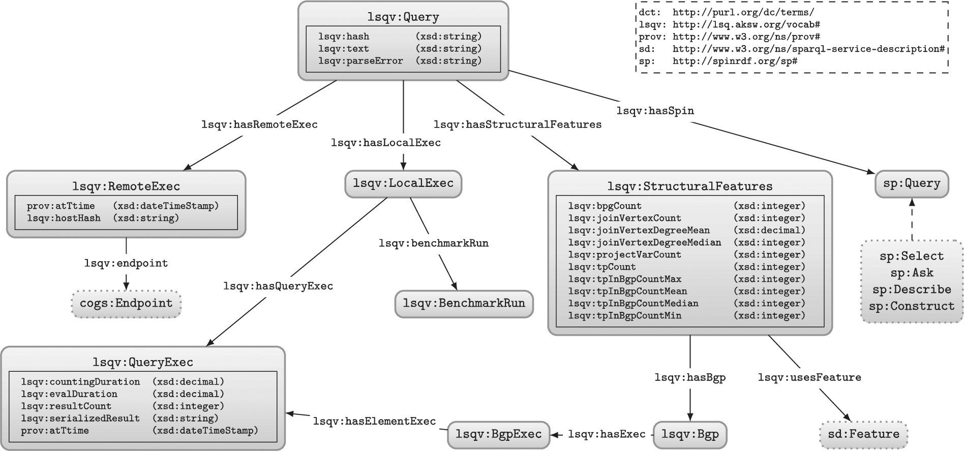 |
D4 Linked Data Compatibility | URIs should be dereferenceable so as to abide by the Linked Data Principles. Terms from external well-known vocabularies should be re-used where appropriate. Links to other datasets should be provided. |
It is important to note that some of these desiderata are incompatible. For example, D2 is in direct conflict with D1 as adding more meta-data for queries can increase generality, but decreases conciseness. D2 can also be seen as being in conflict with D3 and D4, as D3 can be achieved by adding “shortcut” representations for common needs, while D4 requires the addition of links to external datasets, both of which reduce conciseness. Consequently, the data model must find a balance between providing a detailed description of each query, being useful for various purposes, and keeping the overall dataset relatively concise and manageable.
In Fig. 1 we provide an overview of the model used to represent queries in RDF, while in Listing 1 we provide a snippet of the top-level data generated for a query found in the SWDF logs.33 We now discuss the groups of features described for each query.
Query instance We define a “query” to be uniquely identified by the syntactic query string (independently of the endpoint, the particular execution, etc.). We type these queries with lsqv:Query. Instances of this class are linked to the query string using lsqv:text, and to various instances of local and remote executions. Other links are provided to other resources that capture further details of the static features of the query, its structure, as well as runtime statistics of its local execution (on our server) as information about its remote execution (on the original server).
Listing 1.
An example LSQ/RDF representation of a SPARQL query in Turtle syntax
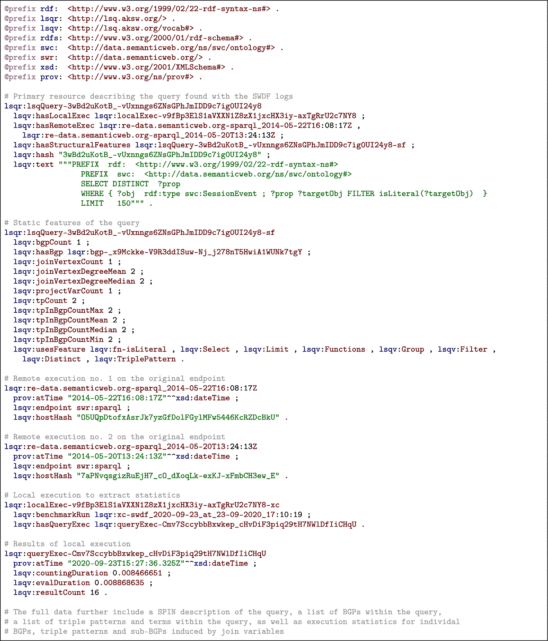
Static features Next we define some static features of the query, independent of the dataset over which it is evaluated. These include links to its individual join variables, triple patterns, and basic graph patterns; the SPARQL features that is uses; its number of projected variables, basic graph patterns, join variables, triple patterns; the maximum, mean and median degree of its join variables; and the maximum and minimum size of its basic graph patterns. The triple patterns and basic graph patterns themselves link to the SPIN representation of the query included in the description (and discussed presently); the triple patterns, in turn, link to the resources used by the query. The join variables, on the other hand, are described separately, indicating the degree of the variable and type of join [81] it induces.
SPIN representation While the static features aim to capture some high-level descriptions of the query that may be of interest to specific use cases, some details may be missing. In the interest of generality, we also include for each query a SPARQL Inferencing Notation (SPIN) [48] representation of the query, which essentially captures a fine-grained translation of the SPARQL query to RDF. This SPIN encoding can be translated back to a SPARQL query equivalent to the original.44
Remote execution(s) Next, individual queries are associated with one or more executions on the original endpoint, including a timestamp of when the query was executed, as well as an anonymised ID for the client – based on their cryptographically-hashed and salted I.P. – to identify which queries are run by the same agent.55 The remote execution is also linked to the originating endpoint using lsqv:endpoint.66 Given that these meta-data constitute provenance for the query, we use the PROV Ontology (PROV-O) [51] for modelling the time, date and agent involved in the remote execution.
Local execution In most cases, the log of the remote executions will not provide statistics about the execution of the query in terms of how many results were returned, how long it took, how selective were the individual patterns, and so forth. Hence we re-execute the queries offline against the original dataset to generate runtime statistics about the query. Local executions were run on a machine with 64 core Intel(R) Xeon(R) CPU E5-2683 v4 @ 2.10 GHz, and 528 GB RAM running Ubuntu 18.04.5 LTS using Virtuoso 7.2.77 Due to the large number of queries to evaluate, we set a query timeout of one minute. The statistics generated include the number of results and the runtime for the query, as well as the number of results and the selectivity for each individual triple pattern.88 Runtime statistics are computed in a controlled environment that abstract away external factors such as the load on the endpoint server, etc.; however, due to the costs involved in evaluating such queries, we compute these only for one query engine, namely Virtuoso 7.2, where runtime estimates may thus vary for other engines.
Summary The meta-data described in this section aim to strike a balance in terms of the four desiderata mentioned previously. In terms of Generality, we provide detailed meta-data for static query features, for provenance, and for runtime query statistics. In terms of Conciseness, though the detailed meta-data do require potentially many triples to be encoded for each query, we take steps to reduce this number by re-using resources insofar as appropriate where, for example, each unique query string is encoded once per log, with one set of static features, one SPIN representation, and one set of local executions, being subsequently linked to its different remote executions (rather than duplicate the former meta-data each time the same query string appears in the log). In terms of Usability, we provide some “shortcut triples” that allow for quickly finding queries of interest; for example, the static features of the query are largely of this form, where all such meta-data could in principle be computed from the SPIN representation, but using rather complex SPARQL queries over LSQ; the static query features are thus presented to make it easier to find queries, for example, with a certain range of numbers of triple patterns, or queries using DISTINCT and GROUP BY, etc. We will discuss Linked Data Compatibility in the section that follows.
4.Publication
The LSQ dataset is published as Linked Data. Before describing the current contents of LSQ, we discuss in more detail how LSQ has been published.
Access methods We provide a number of ways to access LSQ. Firstly, following Linked Data principles, all IRIs under the lsqr: namespace are made dereferenceable using a 303 Redirect; this is implemented with LodView99 and supports content negotiation. A SPARQL endpoint is provided for querying LSQ 2.0. Table 1 lists the locations for these access methods.
Table 1
Locations from which LSQ can be accessed including an example Linked Data IRI, the vocabulary, dumps, the SPARQL endpoint, as well as locations where LSQ is indexed, including DataHub, Linked Open Vocabularies (LOV) and prefix.cc
| Method | Location |
| Linked Data IRIs | http://lsq.aksw.org/lsqQuery-3wBd2uKotB_-vUxnngs6ZNsGPhJmIDD9c7ig0UI24y8 (example) |
| Vocabulary | http://lsq.aksw.org/vocab |
| Dumps | http://lsq.aksw.org/downloads |
| SPARQL Endpoint | http://lsq.aksw.org/sparql |
| Catalogue | Location |
| Datahub | https://datahub.io/dataset/lsq |
| LOV | https://lov.linkeddata.es/dataset/lov/vocabs/lsq |
| prefix.cc | http://prefix.cc/lsqv |
Vocabulary As seen in Fig. 1, we use a mixture of a custom vocabulary in the lsqv: namespace, as well as existing vocabulary where possible. The custom LSQ vocabulary dereferences (via 303 Redirect) to an RDFS/OWL definition of the corresponding terms in Turtle, which includes metadata about authors. The vocabulary meets four of the five stars of Linked Data vocabulary use [46].1010 With respect to external vocabulary, we re-use terms from the SPARQL Inferencing Notation (SPIN) ontology [48], as well as the Provenance Ontology (PROV-O) [51] where possible.
Discoverability The LSQ dataset has been registered in the DataHub catalogue, while the LSQ vocabulary has been listed on Linked Open Vocabularies (LOV) [92] as well as prefix.cc. We provide these locations in Table 1. We also compute and publish meta-data about the LSQ dataset using the Vocabulary of Interlinked Datasets (VoID) [5]. More specifically, we compute a separate VoID description for each log and make the resulting description accessible via both a downloadable file and a named graph of the SPARQL endpoint.
Availability The LSQ dataset has been hosted for over six years (at the time of writing) by the Agile Knowledge Engineering and Semantic Web (AKSW) group. As discussed in Section 7, it has been widely adopted in that time. The dataset is available to all under a CC-BY license. We further make the source code used for generating the LSQ dataset from the raw query logs available on Github https://github.com/AKSW/LSQ.
Table 2
High-level statistics for queries in the LSQ dataset (QE = Query Executions, UQ = Unique Queries, RE = Runtime Error, ZR = Zero Results, SEL = SELECT, CON = CONSTRUCT, DES = DESCRIBE)
| Dataset | QE | UQ | RE | ZR | SEL (%) | CON (%) | DES (%) | ASK (%) |
| Affymetrix | 1,229,339 | 311,096 | 277,983 | 31,659 | 16.47 | 83.21 | 0.02 | 0.30 |
| BioModels | 1,238,375 | 435,232 | 412,984 | 21,692 | 41.18 | 58.75 | 0.00 | 0.06 |
| BIOPORTAL | 1,337,804 | 89,664 | 85,273 | 3,389 | 64.88 | 34.78 | 0.00 | 0.34 |
| CTD | 940,390 | 287,296 | 266,999 | 19,824 | 11.98 | 87.76 | 0.00 | 0.26 |
| DBpedia | 6,535,500 | 4,258,941 | 1,259,972 | 1,755,338 | 69.90 | 3.59 | 25.23 | 1.28 |
| dbSNP | 794,023 | 269,498 | 267,662 | 1,698 | 4.99 | 94.99 | 0.00 | 0.02 |
| DrugBank | 1,613,951 | 379,233 | 372,022 | 6,186 | 46.67 | 52.80 | 0.05 | 0.48 |
| GenAge | 589,211 | 265,067 | 263,205 | 1,661 | 5.55 | 94.43 | 0.00 | 0.02 |
| GenDR | 690,864 | 270,697 | 262,776 | 7,726 | 7.53 | 92.45 | 0.00 | 0.02 |
| GO | 1,839,991 | 121,542 | 88,743 | 30,082 | 98.31 | 0.03 | 0.35 | 1.31 |
| GOA | 3,544,273 | 343,836 | 310,800 | 32,317 | 26.18 | 73.69 | 0.06 | 0.07 |
| HGNC | 1,529,681 | 364,961 | 327,540 | 33,568 | 29.15 | 70.58 | 0.04 | 0.23 |
| iRefIndex | 1,560,704 | 309,777 | 289,546 | 19,858 | 18.10 | 81.88 | 0.00 | 0.02 |
| KEGG | 66,830 | 19,871 | 10,386 | 8,004 | 92.04 | 4.30 | 0.41 | 3.24 |
| LinkedGeoData | 154,884 | 61,897 | 11,028 | 13,990 | 98.58 | 1.00 | 0.02 | 0.40 |
| LinkedSQP | 337,001 | 204,112 | 203,534 | 310 | 0.28 | 99.69 | 0.00 | 0.03 |
| MGI | 1,316,673 | 319,627 | 277,080 | 33,781 | 21.12 | 78.60 | 0.05 | 0.23 |
| NCBIGene | 770,716 | 216,832 | 215,938 | 718 | 8.71 | 91.26 | 0.00 | 0.04 |
| OMIM | 1,506,621 | 335,541 | 290,483 | 44,093 | 22.78 | 76.89 | 0.08 | 0.26 |
| PharmGKB | 94,540 | 24,000 | 14,597 | 8,649 | 60.35 | 39.65 | 0.00 | 0.01 |
| SABIORK | 922,407 | 274,098 | 253,733 | 19,938 | 7.91 | 92.07 | 0.00 | 0.02 |
| SGD | 973,281 | 318,641 | 309,593 | 7,199 | 16.06 | 80.53 | 0.30 | 3.12 |
| SIDER | 599,285 | 277,766 | 274,963 | 1,965 | 9.38 | 90.59 | 0.00 | 0.03 |
| SWDF | 1,415,567 | 101,423 | 30,792 | 36,789 | 73.57 | 0.06 | 26.17 | 0.21 |
| Taxonomy | 7,698,898 | 354,582 | 334,290 | 20,041 | 15.83 | 84.16 | 0.00 | 0.02 |
| Wikidata | 3,298,254 | 844,256 | 520,976 | 150,395 | 95.03 | 0.13 | 0.08 | 4.77 |
| Wormbase | 1,353,316 | 498,170 | 496,325 | 1,660 | 49.33 | 50.66 | 0.00 | 0.01 |
| Overall | 43,952,379 | 11,557,656 | 7,729,223 | 2,312,530 | 36.14 | 57.8 | 1.89 | 0.60 |
5.LSQ 2.0 logs
We now describe the content of the LSQ 2.0 dataset. In order to collect raw SPARQL query logs, we sent mails both to the [email protected] mailing list and to individual providers of endpoints. We also incorporated logs from LSQ 1.0 [77] and a sample of queries from the Wikidata logs [57]. We thus acquired access to the logs of 27 endpoints, 22 of which are part of Bio2RDF release 3 [33].1111 Table 2 provides high-level statistics of the query logs from which we extract the LSQ dataset, including the query executions registered; the unique query strings; the number of queries providing a runtime error, or returning zero results; as well as the percentage of unique queries using SELECT, CONSTRUCT, DESCRIBE or ASK. Aside from the initial log of LSQ, only one log is already publicly available, namely Wikidata [57], of which we include a subset described in our data model.
Affymetrix | is a biomedical Linked Dataset describing probesets found in DNA microarrays [33]. |
BioModels | is a biomedical Linked Dataset describing mathematical models of biological systems [33].1212 |
BioPortal | is a biomedical Linked Dataset cataloguing biomedical ontologies [33]. |
CTD: Comparative Toxicogenomics Database | is a biomedical Linked Dataset that describes how environmental chemicals relate to diseases [33]. |
DBpedia | is a cross-domain Linked Dataset that is primarily extracted from Wikipedia [53]. |
dbSNP: Single Nucleotide Polymorphism Database | is a biomedical Linked Dataset that describes single base nucleotide substitutions and short deletion and insertion polymorphisms [33]. |
DrugBank | is a biomedical Linked Dataset that describes drugs and drug targets [33]. |
GenAge | is a biomedical Linked Dataset that describes human and other genes linked with ageing [33]. |
GenDR: Dietary Restriction Gene Database | is a biomedical Linked Dataset that describes genes associated with dietary restrictions [33]. |
GO: Gene Ontology | is a biomedical ontology that describes gene, gene products, and their functions [33]. |
GOA: Gene Ontology Annotation | is a biomedical Linked Dataset that provides annotations on proteins, RNA and protein complexes [33]. |
HGNC: HUGO Gene Nomenclature Committee | is a biomedical Linked Dataset that describes human gene nomenclature [33]. |
iRefIndex | is a biomedical Linked Dataset that indexes interaction data for proteins [33]. |
KEGG: Kyoto Encyclopedia of Genes and Genomes | is a biomedical Linked Dataset that describes functions of genes and biological systems [33]. |
LinkedGeoData | is a geographical Linked Data extracted primarily from Open Street Map [88]. |
LinkedSQP: Linked Structured Product Labelling | is a biomedical Linked Dataset that contains meta-data about drug labels sourced from DailyMed [33]. |
MGI: Mouse Genome Informatics | is a biomedical Linked Dataset that describes mouse genes, alleles, and strains [33]. |
NCBI Gene | is a biomedical Linked Dataset that describes gene-related information given by the National Center for Biotechnology Information (NCBI) [33]. |
Online Mendelian Inheritance in Man (OMIM) | is a biomedical Linked Dataset that catalogues human genes as well as genetic traits and disorders [33]. |
PharmGKB | is a biomedical Linked Dataset describing how genetic variations impact drug responses [33]. |
SABIORK: System for the Analysis of Biochemical Pathways – Reaction Kinetics | is a biomedical Linked Dataset that describes biochemical reactions [33]. |
SGD: Saccharomyces Genome Database | is a biomedical Linked Dataset describing the biology and genetics of the yeast Saccharomyces cerevisiae [33]. |
SIDER: Side Effect Resource | is a biomedical Linked Dataset describing the side effects of drugs [33]. |
SWDF: Semantic Web Dog Food | is a bibliographical Linked Dataset describing papers, presentations and people participating in top Semantic Web related conferences and workshops [61]. |
Taxonomy: NBCI Taxonomy | is a biomedical Linked Dataset that describes all organisms found in genetic databases [33]. |
Wikidata | is a collaboratively edited knowledge graph hosted by the Wikimedia foundation [57]. |
Wormbase | is a biomedical Linked Dataset that describes the biology and genome of worms [33]. |
6.LSQ 2.0 query statistics
We now look in more detail at the composition of the queries currently included in the LSQ dataset. In particular, we first look at some high-level statistics for queries in the dataset, before looking at the static features of the query, the agents making the queries, as well as runtime statistics computed against the corresponding dataset. Finally we discuss the composition of the LSQ dataset itself.
High-level statistics Table 2 provides a high-level analysis of the queries (both query executions and unique queries) appearing in each of the logs considered. From the overall row, we see that LSQ contains 43.95 million query executions and 11.56 million unique queries, implying that each query is executed, on average, 3.8 times within each log. Of the unique queries, 7.7 million (66.9%) have runtime errors; and 2.3 million (20.0%) have no errors but return empty results. A high ratio of runtime errors come from the Bio2RDF logs. The majority of queries are CONSTRUCT queries (60.0%), followed by SELECT (32.3%), DESCRIBE (7.1%) and ASK (0.5%). We find that CONSTRUCT queries are particularly prevalent on Bio2RDF endpoints, while DESCRIBE queries are particularly prevalent on DBpedia and Wikdata endpoints, possibly due to the use of such queries for dereferencing Linked Data IRIs through the endpoint.
Static features Turning to static features, we first look at the percentages of unique queries without parse errors using different SPARQL features (note that we will analyse joins in BGPs and property paths later). Table 3 provides statistics for the usage of different features of SPARQL. We see that FILTER is among the most widely used features, along with SPARQL functions and expressions (note that almost all filters use such expressions). This feature is followed by DISTINCT and other solution modifiers, UNION, OPTIONAL, etc. Notably these are all SPARQL 1.0 features. The SERVICE keyword is commonly used on Wikidata since the Wikidata Query Service provides a custom service for retrieving multilingual labels as preferred/available.
Table 3
Percentage of unique queries without parse errors using the specified SPARQL feature (Sol. Mod. includes the solution modifiers ORDER BY, OFFSET, and LIMIT; Agg. includes aggregation features GROUP BY, HAVING, AVG, SUM, COUNT, MAX, and MIN; Neg. includes MINUS, NOT EXISTS, and EXISTS; Bind. includes VALUES and BINDING; Graph includes FROM, FROM NAMED, and GRAPH; Func. includes SPARQL functions and expressions)
| Dataset | UNION | OPTIONAL | DISTINCT | FILTER | REGEX | SERVICE | Sub-Q. | Sol. M. | Agg. | Neg. | Bind. | Graph | Func. |
| Affymetrix | 3.68 | 0.02 | 7.64 | 83.30 | 0.15 | 0.01 | 0.06 | 4.85 | 0.36 | 0.00 | 0.01 | 0.69 | 83.30 |
| BioModels | 2.64 | 0.01 | 0.18 | 94.32 | 0.06 | 0.00 | 0.01 | 0.12 | 0.10 | 0.00 | 0.00 | 0.03 | 94.32 |
| BIOPORTAL | 1.50 | 0.06 | 0.05 | 37.95 | 2.23 | 0.01 | 0.01 | 0.21 | 34.10 | 0.00 | 0.00 | 34.26 | 37.95 |
| CTD | 3.99 | 0.02 | 0.37 | 88.06 | 0.06 | 0.04 | 0.01 | 3.57 | 0.13 | 0.00 | 0.01 | 3.21 | 88.06 |
| DBpedia | 28.68 | 19.97 | 22.22 | 29.87 | 4.10 | 0.00 | 2.22 | 8.92 | 9.98 | 0.00 | 1.11 | 0.01 | 29.87 |
| dbSNP | 0.05 | 0.01 | 0.10 | 94.87 | 0.00 | 0.05 | 0.01 | 0.13 | 0.07 | 0.00 | 0.00 | 0.09 | 94.87 |
| DrugBank | 2.58 | 15.55 | 12.37 | 54.67 | 1.81 | 0.10 | 0.02 | 9.31 | 2.59 | 0.00 | 0.01 | 2.73 | 54.67 |
| GenAge | 0.00 | 0.01 | 0.08 | 94.37 | 0.00 | 0.00 | 0.01 | 0.06 | 0.07 | 0.00 | 0.00 | 0.02 | 94.37 |
| GenDR | 0.01 | 0.01 | 0.07 | 96.55 | 0.00 | 0.01 | 0.01 | 0.06 | 0.07 | 0.00 | 0.00 | 0.02 | 96.55 |
| GO | 9.08 | 0.16 | 20.98 | 18.82 | 5.92 | 0.89 | 0.07 | 3.86 | 0.08 | 0.00 | 0.01 | 0.02 | 18.82 |
| GOA | 4.17 | 0.01 | 5.00 | 84.76 | 9.15 | 0.86 | 0.03 | 0.71 | 0.09 | 0.00 | 0.00 | 0.44 | 84.76 |
| HGNC | 3.16 | 0.02 | 5.00 | 84.12 | 0.04 | 0.03 | 0.02 | 1.20 | 0.44 | 0.00 | 0.00 | 0.47 | 84.12 |
| iRefIndex | 9.99 | 1.00 | 0.86 | 83.37 | 2.29 | 0.01 | 0.01 | 0.87 | 0.12 | 0.00 | 0.00 | 0.74 | 83.37 |
| KEGG | 11.64 | 1.13 | 54.91 | 7.22 | 2.86 | 0.07 | 0.04 | 42.95 | 1.02 | 0.00 | 0.01 | 0.79 | 7.22 |
| LinkedGeoData | 1.15 | 19.13 | 9.24 | 18.06 | 2.61 | 0.01 | 7.64 | 30.75 | 37.57 | 0.00 | 0.52 | 2.52 | 18.06 |
| LinkedSQP | 0.00 | 0.01 | 0.00 | 99.76 | 0.00 | 0.00 | 0.01 | 0.05 | 0.07 | 0.00 | 0.00 | 0.03 | 99.76 |
| MGI | 3.57 | 0.02 | 6.99 | 79.43 | 0.43 | 0.01 | 0.03 | 2.98 | 0.57 | 0.00 | 0.05 | 0.64 | 79.43 |
| NCBIGene | 0.02 | 0.01 | 0.17 | 91.53 | 0.02 | 0.03 | 0.01 | 2.72 | 0.22 | 0.00 | 0.00 | 2.61 | 91.53 |
| OMIM | 3.52 | 1.10 | 4.90 | 80.83 | 0.31 | 0.39 | 0.04 | 5.62 | 0.93 | 0.00 | 0.01 | 1.09 | 80.83 |
| PharmGKB | 33.05 | 0.00 | 42.22 | 47.92 | 0.28 | 0.13 | 0.01 | 43.40 | 0.07 | 0.00 | 0.00 | 1.14 | 47.92 |
| SABIORK | 4.15 | 0.01 | 0.12 | 92.00 | 0.00 | 0.00 | 0.01 | 0.17 | 0.09 | 0.00 | 0.00 | 0.05 | 92.00 |
| SGD | 1.63 | 0.01 | 6.73 | 80.06 | 0.09 | 0.03 | 0.04 | 4.38 | 3.87 | 0.00 | 0.00 | 4.24 | 80.06 |
| SIDER | 0.02 | 0.01 | 7.44 | 90.87 | 0.00 | 0.03 | 0.01 | 7.42 | 0.09 | 0.00 | 0.00 | 0.73 | 90.87 |
| SWDF | 40.13 | 34.08 | 53.16 | 2.34 | 0.87 | 0.04 | 0.10 | 31.45 | 1.08 | 0.00 | 0.01 | 32.32 | 2.34 |
| Taxonomy | 3.19 | 0.01 | 0.04 | 92.91 | 0.04 | 0.00 | 0.01 | 0.35 | 0.25 | 0.00 | 0.00 | 0.44 | 92.91 |
| Wikidata | 9.27 | 29.21 | 15.32 | 26.48 | 1.13 | 54.38 | 7.44 | 40.72 | 7.99 | 0.00 | 8.99 | 0.00 | 26.48 |
| Wormbase | 14.16 | 4.46 | 0.12 | 69.92 | 9.69 | 1.58 | 0.00 | 0.27 | 0.63 | 0.00 | 0.00 | 0.82 | 69.92 |
| Overall | 7.22 | 4.67 | 10.23 | 67.57 | 1.63 | 2.17 | 0.66 | 9.14 | 3.77 | 0.00 | 0.34 | 3.34 | 67.57 |
Next, in Table 4, we provide three types of statistics about the basic graph patterns and property path features used. First, we present the unique number of subject, predicate and object terms used in the BGPs of the logs in order to characterise their diversity. We see that DBpedia, LinkedGeoData and Wikidata offer the most diversity, particularly in terms of predicates found in the queries. Second, we present the percentage of queries with different types of joins in the basic graph patterns [81]. Each join variable in a basic graph pattern is analysed in order to understand how they connect triple patterns. We say that a join vertex has an “outgoing link” if it appears as a subject of a triple pattern, and that it has an “incoming link” if it appears as predicate or object. The join types are then defined as follows:
Star | has multiple outgoing but no incoming links. |
Path | has one incoming and one outgoing link. |
Hybrid | has at least one incoming and outgoing link and three or more links overall. |
Sink | has multiple incoming but no outgoing links. |
These statistics may be helpful for consumers to choose which dataset/log to work with. For example, for the purposes of benchmarking joins, a dataset such as LinkedGeoData or Wikidata may be chosen as most queries feature joins; in order to benchmark or analyse property paths, DBpedia or Wikidata may be chosen as they use this feature more frequently; etc.
Table 4
Analysis of basic graph patterns and property paths including number of unique subject/predicate/object terms, percentage of unique queries containing different types of joins (a query may contain multiple join types), and number of queries using different types of property path expressions (/ denotes concatenation, ^ denotes inverse, * denotes zero-or-more; + denotes one-or-more; | denotes disjunction
| Dataset | BGP Terms | Join Types (%) | Prop. Path Features | ||||||||||
| Subj. | Pred. | Obj. | Star | Hyb. | Path | Sink | None | / | ^ | * | + | | | |
| Affymetrix | 17,912 | 432 | 27,398 | 2.36 | 0.16 | 0.03 | 0.10 | 97.57 | 2 | 0 | 0 | 0 | 1 |
| BioModels | 14,055 | 347 | 120,148 | 37.22 | 0.10 | 0.01 | 0.04 | 62.71 | 2 | 0 | 0 | 0 | 1 |
| BIOPORTAL | 9,275 | 130 | 6,275 | 36.26 | 34.22 | 0.01 | 53.08 | 44.60 | 1 | 0 | 0 | 0 | 1 |
| CTD | 14,927 | 276 | 22,320 | 1.72 | 0.19 | 0.04 | 0.16 | 98.21 | 3 | 1 | 0 | 0 | 1 |
| DBpedia | 912,943 | 10,842 | 1,104,732 | 29.38 | 7.06 | 1.71 | 15.48 | 69.56 | 49,660 | 39,039 | 271 | 7,582 | 32,709 |
| dbSNP | 12,825 | 112 | 6,069 | 2.10 | 0.06 | 0.01 | 0.04 | 97.86 | 2 | 0 | 0 | 0 | 1 |
| DrugBank | 37,578 | 989 | 34,601 | 33.39 | 16.81 | 2.01 | 7.50 | 64.44 | 8 | 0 | 1 | 0 | 1 |
| GenAge | 2,666 | 113 | 11,875 | 4.30 | 0.04 | 0.01 | 0.01 | 95.66 | 2 | 0 | 0 | 0 | 1 |
| GenDR | 5,664 | 104 | 705 | 4.22 | 4.17 | 0.01 | 0.01 | 95.74 | 3 | 0 | 0 | 0 | 1 |
| GO | 35,504 | 394 | 59,362 | 16.51 | 0.90 | 0.87 | 1.31 | 83.14 | 4 | 2 | 0 | 0 | 1 |
| GOA | 33,593 | 204 | 22,044 | 8.06 | 0.05 | 0.02 | 0.02 | 91.89 | 5 | 0 | 0 | 0 | 1 |
| HGNC | 23,430 | 414 | 36,857 | 15.72 | 1.53 | 0.02 | 4.30 | 84.21 | 2 | 0 | 0 | 0 | 1 |
| iRefIndex | 20,067 | 171 | 28,069 | 9.09 | 0.35 | 0.01 | 1.50 | 90.85 | 2 | 0 | 0 | 0 | 1 |
| KEGG | 5,620 | 251 | 8,964 | 7.24 | 1.67 | 0.51 | 0.93 | 92.08 | 3 | 0 | 0 | 0 | 1 |
| LinkedGeoData | 13,498 | 5,991 | 2,628 | 49.51 | 24.15 | 0.04 | 34.27 | 41.28 | 672 | 78 | 0 | 0 | 9 |
| LinkedSQP | 326 | 55 | 144 | 0.05 | 0.03 | 0.02 | 0.00 | 99.91 | 2 | 0 | 0 | 0 | 1 |
| MGI | 28,702 | 391 | 23,867 | 2.13 | 1.36 | 0.15 | 0.56 | 97.79 | 5 | 0 | 0 | 0 | 1 |
| NCBIGene | 11,753 | 254 | 4,427 | 2.16 | 0.20 | 0.02 | 0.18 | 97.79 | 3 | 0 | 1 | 0 | 1 |
| OMIM | 23,504 | 623 | 50,229 | 7.00 | 4.57 | 0.34 | 3.95 | 92.52 | 10 | 0 | 0 | 0 | 3 |
| PharmGKB | 1,099 | 83 | 13,548 | 8.03 | 50.69 | 0.82 | 1.83 | 47.97 | 0 | 0 | 0 | 0 | 1 |
| SABIORK | 14,224 | 156 | 19,775 | 0.70 | 0.04 | 0.02 | 0.01 | 99.25 | 2 | 0 | 0 | 0 | 1 |
| SGD | 7,228 | 508 | 13,460 | 6.83 | 5.65 | 0.03 | 4.02 | 93.06 | 2 | 0 | 0 | 0 | 1 |
| SIDER | 8,792 | 152 | 3,589 | 0.53 | 0.08 | 0.02 | 0.04 | 99.43 | 6 | 0 | 0 | 0 | 1 |
| SWDF | 25,640 | 420 | 10,823 | 32.05 | 7.27 | 3.34 | 0.95 | 58.62 | 94 | 22 | 0 | 0 | 17 |
| Taxonomy | 16,201 | 207 | 97,298 | 22.54 | 0.23 | 0.01 | 0.21 | 77.41 | 6 | 0 | 0 | 0 | 1 |
| Wikidata | 47,871 | 11,779 | 263,974 | 46.63 | 17.59 | 4.98 | 12.05 | 41.20 | 134,811 | 2,944 | 3,838 | 0 | 23,525 |
| Wormbase | 53,807 | 148 | 24,083 | 39.40 | 5.13 | 4.47 | 5.07 | 60.55 | 2 | 0 | 0 | 0 | 1 |
| Overall | 1,398,704 | 35,546 | 2,017,264 | 15.74 | 6.58 | 0.72 | 5.47 | 80.56 | 185,314 | 42,086 | 4,111 | 7,582 | 56,285 |
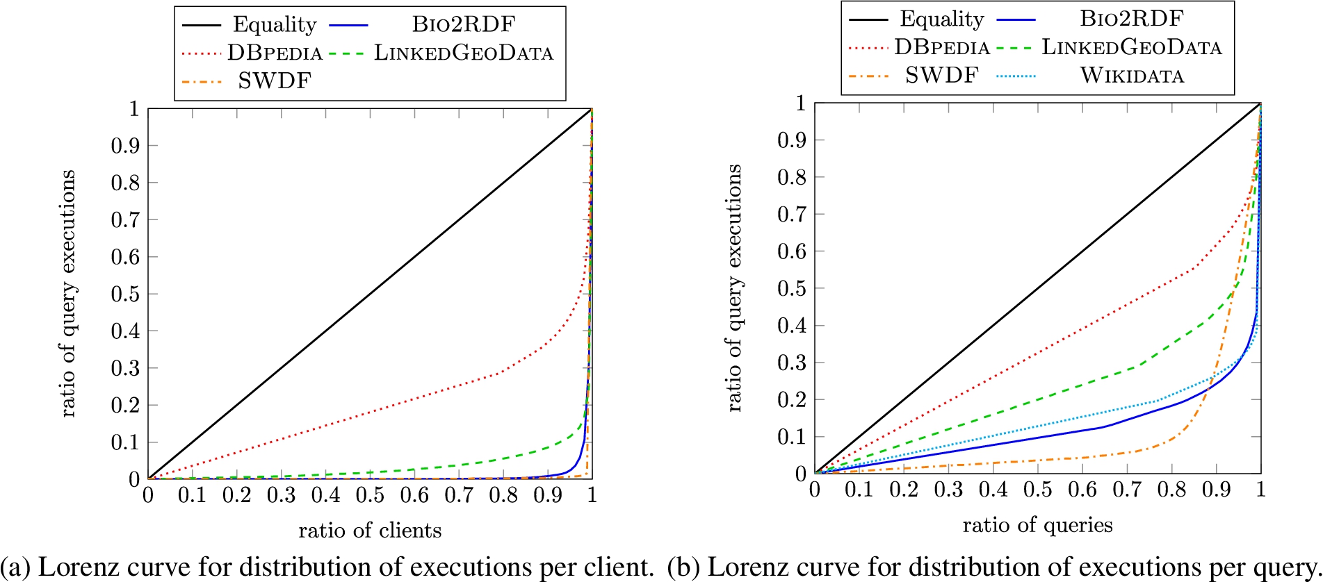
Provenance: Executions and agents Next we look at how many clients (anonymised IPs) and unique queries underlie the executions registered in order to compare the diversity of the different datasets. Note that client information is not available for Wikidata. In Fig. 2(a) and Fig. 2(b), we present Lorenz curves for the number of executions per client and per query, respectively.1313 We present results for Bio2RDF together as one series to ensure better readability. In general, we see a skew in the graph away from the equality curve towards the bottom-left corner, meaning that a small number of clients/queries are involved in a large number of executions. The skew is more evident in the case of clients, and particularly for the SWDF and Bio2RDF datasets; thus consumers of LSQ 2.0 should be aware that a high ratio of queries from these datasets come from a small number of clients (likely bots). DBpedia is the most diverse in terms of clients and queries.
Fig. 2.
Lorenz curves for the LSQ dataset
Static and runtime statistics Next, in order to characterise how complex the queries are to evaluate, in Table 5 we present some relevant static and runtime statistics, where static statistics can be computed from the query string, while runtime statistics require evaluating the query locally (only queries that were successfully run are counted; see Table 2 for statistics on runtime errors). Regarding runtimes, we recall that these were run with a one minute timeout, which represents the max runtime. We see that LinkedGeoData contains the most costly queries to run, which appears to correlate with larger result sizes and a larger mean join-vertex degree. Relatively high runtimes are also seen for the KEGG dataset. The simplest queries to run are found in the GenAge, GenDR and Taxonomy datasets. These results suggest, for example, that LinkedGeoData might be more suitable for consumers looking for a challenging benchmark.
Table 5
Comparison of the mean values of runtime statistics across all query logs (PVs = Project Variables, BGPs = Basic Graph Patterns, TPs = Triple Patterns, JVs = Join Vertices, MJVD = Mean Join Vertex Degree, MTPS = Mean Triple Pattern Selectivity)
| Dataset | Static Statistics (mean) | Runtime Statistics (mean) | ||||||
| PVs | BGPs | TPs | JVs | MJVD | MTPS | Result Size | Runtime (sec) | |
| Affymetrix | 1.93 | 1.06 | 1.10 | 0.03 | 0.06 | 0.82 | 12708.39 | 0.084 |
| BioModels | 1.24 | 1.04 | 1.42 | 0.37 | 0.75 | 0.57 | 4896.67 | 0.011 |
| BIOPORTAL | 1.16 | 1.03 | 1.94 | 1.43 | 1.12 | 0.54 | 1699.48 | 0.004 |
| CTD | 2.56 | 1.05 | 1.08 | 0.02 | 0.04 | 0.85 | 24354.24 | 0.102 |
| DBpedia | 2.78 | 2.37 | 3.23 | 0.93 | 0.66 | 0.01 | 114038.38 | 0.164 |
| dbSNP | 1.09 | 1.02 | 1.04 | 0.02 | 0.04 | 0.97 | 757108.37 | 0.009 |
| DrugBank | 2.61 | 1.05 | 1.93 | 0.69 | 0.91 | 0.66 | 119759.38 | 0.007 |
| GenAge | 1.88 | 1.00 | 1.09 | 0.04 | 0.13 | 0.99 | 1642.84 | 0.003 |
| GenDR | 2.73 | 1.00 | 1.08 | 0.08 | 0.09 | 0.97 | 83.50 | 0.003 |
| GO | 1.46 | 1.10 | 1.37 | 0.22 | 0.38 | 0.02 | 93806.20 | 0.046 |
| GOA | 1.87 | 1.03 | 1.12 | 0.08 | 0.16 | 0.85 | 7692.26 | 0.016 |
| HGNC | 1.91 | 1.05 | 1.29 | 0.23 | 0.35 | 0.80 | 2419.43 | 0.019 |
| iRefIndex | 2.92 | 1.13 | 1.43 | 0.19 | 0.25 | 0.82 | 32200.76 | 0.077 |
| KEGG | 2.27 | 1.15 | 1.31 | 0.13 | 0.18 | 0.33 | 175469.53 | 3.862 |
| LinkedGeoData | 2.27 | 1.16 | 2.62 | 1.10 | 1.76 | 0.15 | 11055973.09 | 6.788 |
| LinkedSQP | 2.01 | 1.00 | 1.00 | 0.00 | 0.00 | 1.00 | 9503.41 | 0.014 |
| MGI | 2.04 | 1.04 | 1.11 | 0.05 | 0.06 | 0.84 | 2050.76 | 0.178 |
| NCBIGene | 1.39 | 1.02 | 1.04 | 0.03 | 0.04 | 0.95 | 10731.33 | 0.021 |
| OMIM | 1.83 | 1.07 | 1.26 | 0.17 | 0.18 | 0.77 | 3505.54 | 0.020 |
| PharmGKB | 1.96 | 1.34 | 2.48 | 1.06 | 1.08 | 0.39 | 255.61 | 0.017 |
| SABIORK | 2.96 | 1.05 | 1.06 | 0.01 | 0.02 | 0.88 | 1610.77 | 0.005 |
| SGD | 1.45 | 1.12 | 1.96 | 0.35 | 0.18 | 0.58 | 108951.60 | 0.058 |
| SIDER | 1.34 | 1.00 | 1.01 | 0.01 | 0.01 | 0.98 | 9703.86 | 0.010 |
| SWDF | 4.04 | 3.37 | 3.97 | 0.45 | 0.92 | 0.03 | 37362.67 | 0.007 |
| Taxonomy | 1.77 | 1.17 | 1.53 | 0.23 | 0.59 | 0.69 | 1928.75 | 0.004 |
| Wikidata | 3.00 | 2.47 | 4.73 | 1.06 | 1.81 | 0.00 | 17817773.63 | 0.412 |
| Wormbase | 1.56 | 1.25 | 2.05 | 0.65 | 0.87 | 0.98 | 9888.61 | 0.007 |
| Overall | 2.07 | 1.26 | 1.71 | 0.35 | 0.47 | 0.65 | 1126559.96 | 0.440 |
LSQ dataset statistics The LSQ 2.0 dataset, describing 43.95 million executions of 11.56 million unique queries, contains 1.24 billion triples, split into 27 named graphs (one for each of the datasets listed).1414
7.LSQ adoption
In this section we present how LSQ has been adopted since its initial release with four logs in 2015. We organise this discussion following the motivational use cases we originally envisaged, as presented in Section 2. Table 6 provides an overview of the research works that have used LSQ, and the relevant use case(s) that they target. We now discuss these works in more detail; note that in the case of works that relate to multiple use cases, we will discuss them once in what we identify to be the “primary” related use case. We further discuss some works that have used the LSQ dataset for use cases beyond the six we had originally envisaged.
Table 6
Research works making use of the LSQ dataset since its initial release, ordered by year and then alphabetically by author name, with relevant use cases indicated (UC1: Custom Benchmarks; UC2: SPARQL Adoption; UC3: Caching; UC4: Usability; UC5: Optimisation; UC6: Meta-Querying)
| Name | Year | UC 1 | UC 2 | UC 3 | UC 4 | UC 5 | UC 6 | Other |
| Saleem et al. [79] | 2015 | ✓ | ||||||
| Arenas et al. [11] | 2016 | ✓ | ✓ | |||||
| Benedetti and Bergamaschi [17] | 2016 | ✓ | ||||||
| Georgala et al. [39] | 2016 | ✓ | ||||||
| Han et al. [41] | 2016 | ✓ | ✓ | |||||
| Hernandez et al. [42] | 2016 | ✓ | ||||||
| Knuth et al. [49] | 2016 | ✓ | ✓ | |||||
| Rico et al. [71] | 2016 | ✓ | ||||||
| Schoenfisch and Stuckenschmidt [85] | 2016 | ✓ | ✓ | |||||
| Song et al. [87] | 2016 | ✓ | ✓ | |||||
| Bonifati et al. [21] | 2017 | ✓ | ✓ | |||||
| Dellal et al. [31] | 2017 | ✓ | ||||||
| Fokou et al. [37] | 2017 | ✓ | ||||||
| Stegemann and Ziegler [89] | 2017 | ✓ | ✓ | ✓ | ||||
| Thakkar et al. [90] | 2017 | ✓ | ||||||
| Akhtar et al. [2] | 2018 | ✓ | ✓ | |||||
| Bonifati et al. [22] | 2018 | ✓ | ✓ | |||||
| Darari et al. [29] | 2018 | ✓ | ||||||
| Martens and Trautner [58] | 2018 | ✓ | ||||||
| Salas and Hogan [76] | 2018 | ✓ | ✓ | |||||
| Saleem et al. [78] | 2018 | ✓ | ||||||
| Saleem et al. [80] | 2018 | ✓ | ||||||
| Varga et al. [94] | 2018 | ✓ | ||||||
| Viswanathan et al. [97] | 2018 | ✓ | ||||||
| Akhtar et al. [3] | 2019 | ✓ | ✓ | |||||
| Cheng and Hartig [26] | 2019 | ✓ | ✓ | ✓ | ||||
| Fafalios and Tzitzikas [34] | 2019 | ✓ | ||||||
| Fernandez et al. [35] | 2019 | ✓ | ||||||
| Potoniec [69] | 2019 | ✓ | ✓ | |||||
| Saleem et al. [83] | 2019 | ✓ | ||||||
| Thost and Dolby [91] | 2019 | ✓ | ✓ | |||||
| Wang et al. [99] | 2019 | ✓ | ||||||
| Savafi et al. [75] | 2019 | ✓ | ||||||
| Singh et al. [86] | 2019 | ✓ | ✓ | |||||
| Azzam et al. [15] | 2020 | ✓ | ||||||
| Bigerl et al. [18] | 2020 | ✓ | ||||||
| Bonifati et al. [24] | 2020 | ✓ | ✓ | ✓ | ||||
| Figueira et al. [36] | 2020 | ✓ | ✓ | |||||
| Jian et al. [47] | 2020 | ✓ | ✓ | |||||
| Zhang et al. [102] | 2020 | ✓ | ✓ | |||||
| Aebeloe et al. [1] | 2021 | ✓ | ✓ | |||||
| Almendros-Jimenez et al. [6] | 2021 | ✓ | ✓ | |||||
| Azzam et al. [14] | 2021 | ✓ |
Table 6
(Continued)
| Name | Year | UC 1 | UC 2 | UC 3 | UC 4 | UC 5 | UC 6 | Other |
| Davoudian et al. [30] | 2021 | ✓ | ||||||
| Desouki et al. [32] | 2021 | ✓ | ||||||
| Röder et al. [74] | 2021 | ✓ | ||||||
| Wang et al. [98] | 2021 | ✓ | ✓ |
UC1: Custom Benchmarks LSQ has been adopted in various works for creating custom benchmarks.
– Saleem et al. [79] present a framework for generating benchmarks that can be used to evaluate SPARQL endpoints under typical workloads; the benchmarks generate query types depending on the features of the queries submitted to the endpoint, where LSQ is used for testing.
– Later works by Saleem et al. further propose frameworks for generating benchmarks from LSQ for the purposes of evaluating query containment [80,82] and federated query evaluation [78], as well as comparing existing SPARQL benchmarks against LSQ in order to understand how representative they are of real workloads [83].
– Hernández et al. [42] present an empirical study of the efficiency of graph database engines for answering SPARQL queries over Wikidata; they refer to LSQ to verify that the query shapes considered for evaluation correspond with other analyses of real-world SPARQL queries.
– Fernández et al. [35] evaluate various archiving techniques and querying strategies for RDF archives that store historical data; in their evaluation, they select the 200 most frequent triple patterns from the DBpedia query set in LSQ.
– Azzam et al. [15] use LSQ for retrieving highly-demanding queries from the dataset in order to evaluate their system for dividing the load processed by different SPARQL servers.
– Bigerl et al. [18] develop a tensor-based triple store, where they used LSQ as input to the FEASIBLE framework to generate a custom benchmark.
– Azzam et al. [14] present a system that dynamically delegates query processing load between clients and servers. The authors use the Linked Data Fragments client/server approach improving it with the aforementioned technique and use 16 queries from LSQ to complement their evaluation.
– Davoudian et al. [30] present a system that partitions graphs depending on the access frequency to their nodes. In this way the system implements workload-aware partitioning. The authors use LSQ for evaluating their approach.
– Desouki et al. [32] propose a method to generate synthetic benchmark data. To generate these synthetic data they use other RDF graphs available, such as SWDF and DBpedia 2016. They benchmark their approach using queries from LSQ.
– Röder et al. [74] develop a method to predict the performance of knowledge graph query engines; to do so the authors use a stochastic generation model that is able to generate graphs of arbitrary sizes similar to the input graph. They use LSQ as a benchmark of real-world queries.
UC2: SPARQL adoption Other works have used LSQ to understand how SPARQL is being used in practice.
– Han et al. [41] provide a statistical analysis of the queries of LSQ, surveying both syntactic features, such as the number of triple patterns, the SPARQL features used, the frequency of well-designed patterns; as well as semantic properties, such as montonicity, weak-monotonicity, non-monotonicity and satisfiability.
– Bonifati et al. [21,22] conduct detailed analysis of the queries in various logs, including LSQ; they study a variety of phenomena in these queries, including their shape, their (hyper)treewidth, common abstract patterns found in the property paths, “streaks” that represent a sequence of user reformulations from a seed query, and more besides.
UC3: Caching LSQ can also be used to simulate real workloads for systems that explore caching techniques.
– Knuth et al. [49] propose a middleware component to which applications register and get notifications when the results of their SPARQL queries change; the authors study the problem of scheduling refresh queries for a large number of registered queries and use LSQ to validate their approach.
– Akhtar et al. [2,3] propose an approach to capture changes in an RDF dataset and update a cache system in front of the SPARQL endpoint exposing that data; their approach consists of a change metric that quantifies the changes in an RDF dataset, and a weighting function that assigns importance to recent changes; they use LSQ to verify their approach for real workloads.
– Salas and Hogan [76] propose a method for query canonicalisation, which consists in mapping congruous queries – i.e., queries that are equivalent modulo variable names – to the same query string; their main use case is to increase the hit rate of SPARQL caches, where they use LSQ to test efficiency on real-world queries and to see how many congruent queries can be found in real workloads.
– Savafi et al. [75] study SPARQL adoption using LSQ so they can later provide queries to summarise the Knowledge Graphs such that they can be more efficiently accessed from and stored on mobile devices with limited resources.
UC4: Usability LSQ also has applications for improving the usability of SPARQL endpoints.
– Arenas et al. [11] propose a method for reverse-engineering SPARQL queries, which attempts to construct a query that will return a given set of positive examples as results, but not a second set of negative examples; the authors use LSQ to show that the approach scales well in the data size, number of examples, and in the size of the smallest query that fits the data.
– Benedetti and Bergamaschi [17] present a system (LODeX) that allows users to explore SPARQL endpoints more easily through a formal model defined over the endpoint schema; they show that LODeX is able to generate 77.6% of the 5 million queries contained in the original LSQ dataset.
– Dellal et al. [31] proposes query relaxation methods for queries with empty results, based on finding minimal failing subqueries (generating empty results) and maximal succeeding subqueries (generating non-empty results) to aid the user [37]. The paper refers to LSQ to establish that queries with empty results are common in practice.
– Stegemann and Ziegler [89] propose new operators for the SPARQL language that allow for composing path queries more easily; the authors evaluated their approach with a user study and analysis of the extent to which their language is able to express the real-world queries found in LSQ.
– Viswanathan et al. [97] propose a different form of query relaxation, which generalises a specific resource to a variable on which specific restrictions are added that correspond to relevant characteristics of the resource; they use LSQ to understand how entities are queried in practice.
– Potoniec [69] proposes an interactive system for learning SPARQL queries from positive and negative examples;1515 he uses the DBpedia queries of LSQ for experiments.
– Wang et al. [99] present an approach for explaining missing results for a SPARQL query – based on answering “why-not” questions that ask why a specific result is not included – to help users refine their initial queries; the authors search LSQ for queries useful for their approach.
– Bonifati et al. [24] analyse “streaks” in DBpedia query logs,1616 where a streak is defined as a sequence of similar queries in chronological order, capturing the idea of a user refining and/or extending an initial query towards a final query.
– Jian et al. [47] use LSQ to evaluate their approach for SPARQL query relaxation (to generalise users’ queries) and query restriction (to refine users’ queries) based on approximation and heuristics.
– Zhang et al. [102] propose a method to model client behaviour when formulating SPARQL queries in order to predict their intent and optimise queries. They use LSQ for their evaluation.
– Almendros-Jimenez et al. [6] present two methods for discovering and diagnosing “wrong” SPARQL queries based on ontology reasoning. They evaluate their approach using LSQ queries.
– Wang et al. [98] focus on providing explanations for SPARQL query similarity measures. The authors provide similarity scores using several explainable models based on Linear Regression, Support Vector Regression, Ridge Regression, and Random Forest Regression. They use LSQ to evaluate their query classification.
UC5: Optimisation The LSQ dataset can also be used to identify and study fragments that are commonly used in practice and can be evaluated efficiently using dedicated algorithms.
– The aforementioned analyses by Han et al. [41] and Bonifati et al. [21,22] suggest that well-designed patterns, queries of bounded treewidth, etc., make for promising fragments.
– In the context of probabilistic Ontology-Based Data Access (OBDA), Schoenfisch and Stuckenschmidt [85] analyse the ratio of safe queries – whose evaluation is tractable in data complexity – versus unsafe queries – whose evaluation is #P-hard; they show that over 97.9% of the LSQ queries are safe, and can be efficiently evaluated.
– Song et al. [87] use LSQ to analyse how nested OPTIONAL clauses affect query response times; they propose a way to approximate solutions for deeply-nested well-designed patterns.
– Martens and Trautner [58] later take the property paths extracted by Bonifati et al. [21] from LSQ and other sources, defining simple transitive expressions that subsume almost all property path expressions seen in practice, while allowing more efficient evaluation than the general case.
– Cheng and Hartig [26] introduce a monotonic version of the OPTIONAL operator to SPARQL called OPT+; a possible downside of the operator is an increase in query result sizes, where they use the LSQ dataset to study how OPTIONAL and OPT+ behave for real-world queries.
– Building upon the work of Martens and Trautner [58], Figueira et al. [36] specifically study the containment problem for restricted classes of Conjunctive Regular Path Queries (CRPQs), which are akin to BGPs with property paths; aside from complexity results, they show the coverage of the different classes for logs that include LSQ [24].
UC6: Meta-querying A handful of works have also used LSQ in the context of meta-querying, where queries are found based on the resources they contain.
– Rico et al. [71] observe that analogous DBpedia properties are often defined in two distinct namespaces – e.g., dbo:birthPlace and dbp:birthPlace – where they propose methods to automatically expand SPARQL queries to capture solutions involving analogous properties; they show that only 0.2% of the DBpedia queries in LSQ mention properties from both namespaces.
– Varga et al. [94] provide an RDF-based metamodel for BI 2.0 systems, which allows for capturing the schema of a dataset, as well as previous queries that have been posed against that dataset by other users; the authors propose to re-use parts of the LSQ vocabulary in their model; they further instantiate their model using LSQ to retrieve queries asked about countries.
Other use cases A number of works have used LSQ (mostly for evaluation) in contexts that were not originally anticipated by the aforementioned use cases.
– Georgala et al. [39] propose a method to predict temporal relations between events represented by RDF resources following Allen’s interval algebra; they use LSQ to validate their approach considering query executions as events.
– Darari et al. [29] present a theoretical framework for augmenting RDF data sources with completeness statements, which allows for reasoning about the completeness of SPARQL query results; they evaluate their method using LSQ.
– Fafalios and Tzitzikas [34] present a query evaluation strategy, called SPARQL-LD, that combines link traversal and query processing at SPARQL endpoints; they provide a method for checking if a SPARQL query can be answered through link traversal, and analyse a large corpus of real SPARQL query logs – including LSQ – for finding the frequency and distribution of answerable and non-answerable query patterns; they also use LSQ to evaluate their approach.
– Singh et al. [86] use the LSQ vocabulary for providing a benchmark for Question Answering over Linked Data. The authors use the LSQ vocabulary to represent the SPARQL query related features prior to generating the benchmark.
– Thost and Dolby [91] present QED: a system for generating concise RDF graphs that are sufficient to produce solutions from a given query, which can be used for benchmarking, for compliance testing, for training query-by-example models, etc.; they apply their system over LSQ queries to generate datasets from DBpedia.
– Aebeloe et al. [1] present a decentralised architecture based on blockchain that allows users to propose updates to faulty or outdated data, tracing back their origin, and query older versions of the data. They use LSQ queries for their evaluation.
Discussion Per Table 6, we see that the original version of LSQ has been used in a wide variety of research works for a variety of purposes. Complementing other SPARQL query logs such as Wikidata’s [57], we believe that LSQ 2.0, with its extended set of queries, will likewise serve as a useful resource to help align the theory and practice of SPARQL research.
8.Conclusions and future directions
In this paper, we have described the Linked SPARQL Queries v.2 (LSQ 2.0) dataset, which represents queries in logs as RDF, allowing clients to quickly find real-world queries that may be of interest to them. We have described a number of use cases for LSQ, including the generation of custom benchmarks, the analysis of how SPARQL is used in practice, the evaluation of caching systems, the exploration of techniques to improve the usability of SPARQL services, the targeted optimisation of queries with characteristics commonly found in real workloads, as well as the ability to find queries relating to specific resources. We then described the model and vocabulary used to represent LSQ, including static features of queries, a SPIN representation, provenance encoding the agents and endpoints from which the query originate, as well as runtime statistics generated through local executions of the queries against their corresponding dataset. We then discussed how LSQ is published, thereafter describing the datasets and queries featured in the current version of LSQ. Finally we discussed how LSQ has been used for research purposes since its initial release in 2015.
As discussed in Section 7, since its initial release, LSQ has been adopted by a variety of research works for a variety of purposes. In terms of future directions, we will look to continue adding further logs with further queries to the dataset. Looking at how LSQ has been adopted in the literature has also revealed ways in which the metadata for LSQ could be extended in a future version, such as to add information about monotonicity and satisfiability [41], or information about (hyper)treewidth [21,22], for example. It may also be useful to provide a canonical version of the query string [76]; this could perhaps be leveraged, for example, when evaluating caching methods. Another useful feature would be to add questions in natural language that verbalise each query, which could be used, for example, in order to create datasets for training and testing question answering systems, as well as enabling users to find relevant queries through keyword search; given the large number of queries in the dataset, an automated approach may be applicable [64].
As discussed by Martens and Trautner [59], query logs allow to bridge the theory and practice of SPARQL. They serve an important role, ensuring that the research conducted by the community is guided by the requirements and trends that emerge in practice. We thus believe that LSQ (2.0) will continue to serve an important role in SPARQL research in the coming years.
Notes
1 http://usewod.org/; retr. 2015/04/14.
3 Note that for the purposes of presentation, we abbreviate some of the details of the query, including the IRIs used to identify local query executions.
4 Given a query Q and dataset D, let
5 A “salt” in cryptography is a privately-held arbitrary string that is combined (e.g., concatenated) with the input being hashed in order to avoid attacks based on precomputed tables (e.g., of common values or, in this case, of a collection of I.P.’s of interest).
6 Although there exist properties called “endpoint” – such as void:sparqlEndpoint or sd:endpoint – the domains of these properties were not query executions, but rather VoID datasets (i.e., sets of RDF triples), or SPARQL services. Though it would be possible to define properties such as lsqv:dataset or lsqv:service and then link a query execution <x> to an endpoint URL <e> with <x> lsqv:dataset [void:sparqlEndpoint <e>], or alternatively <x> lsqv:service [sd:endpoint <e>], this would introduce
7 The configuration used for Virtuoso was MaxQueryMem = 32G, NumberOfBuffers = 20050000, and MaxDirtyBuffers = 20000000.
8 The selectivity of the triple pattern is the ratio of triples from the dataset that it selects.
10 With respect to the fifth star, which requires that our LSQ vocabulary be linked to from external vocabularies, we are not aware of such links, though we do know, for example, that Varga et al. [94] incorporate elements of the LSQ vocabulary within their own Analytical Metadata (AM) model, while Singh et al. [86] also use the LSQ vocabulary within their benchmark.
11 We also acquired logs for the British Museum and UniProt endpoints, but decided to omit them due to having few unique queries.
12 The external SPARQL endpoint is spelt biomedels, and thus the IRIs use this spelling in LSQ 2.0.
13 Lorenz curves visualise (in)equality in distributions for a given quantity over a given set of elements: a coordinate
14 We exclude some named graphs created by Virtuoso.
15 Notably the system is called Learning SPARQL Queries (LSQ).
16 In fact, these logs were gathered directly from OpenLink, though we include discussion since similar analysis could have been applied to the LSQ logs, and LSQ logs where used in other analyses.
Acknowledgements
We thank the OpenLink Software team for hosting the DBpedia SPARQL endpoint and for making the logs available to us. Hogan was supported by Fondecyt Grant No. 1181896 and by ANID – Millennium Science Initiative Program – Code ICN17_002. Buil-Aranda was supported by Fondecyt Iniciación Grant No. 11170714 and by ANID – Millennium Science Initiative Program – Code ICN17_002. This work was also partially supported by the German Federal Ministry of Education and Research (BMBF) within the EuroStars project E!114681 3DFed under the grant no 01QE2114, project RAKI (01MD19012D) and project KnowGraphs (No 860801).
References
[1] | C. Aebeloe, G. Montoya and K. Hose, ColChain: Collaborative linked data networks, in: The Web Conference (WWW), (2021) , pp. 1385–1396, ACM/IW3C2. doi:10.1145/3442381.3450037. |
[2] | U. Akhtar, M.A. Razzaq, U.U. Rehman, M.B. Amin, W.A. Khan, E.-N. Huh and S. Lee, Change-aware scheduling for effectively updating linked open data caches, IEEE Access 6: ((2018) ), 65862–65873. doi:10.1109/ACCESS.2018.2871511. |
[3] | U. Akhtar, A. Sant’Anna and S. Lee, A dynamic, cost-aware, optimized maintenance policy for interactive exploration of linked data, Applied Sciences 9: (22) ((2019) ), 4818. doi:10.3390/app9224818. |
[4] | R. Al-Harbi, I. Abdelaziz, P. Kalnis, N. Mamoulis, Y. Ebrahim and M. Sahli, Accelerating SPARQL queries by exploiting hash-based locality and adaptive partitioning, VLDB J. 25: (3) ((2016) ), 355–380. doi:10.1007/s00778-016-0420-y. |
[5] | K. Alexander, R. Cyganiak, M. Hausenblas and J. Zhao, Describing Linked Datasets with the VoID Vocabulary, 2011, W3C Interest Group Note, https://www.w3.org/TR/void/. |
[6] | J.M. Almendros-Jiménez and A. Becerra-Terón, Discovery and diagnosis of wrong SPARQL queries with ontology and constraint reasoning, Expert Systems with Applications 165: ((2021) ), 113772. doi:10.1016/j.eswa.2020.113772. |
[7] | G. Aluç, O. Hartig, M.T. Özsu and K. Daudjee, Diversified stress testing of RDF data management systems, in: International Semantic Web Conference (ISWC), Springer, (2014) , pp. 197–212. doi:10.1007/978-3-319-11964-9_13. |
[8] | G. Aluç, M.T. Özsu and K. Daudjee, Workload matters: Why RDF databases need a new design, PVLDB 7: (10) ((2014) ), 837–840. doi:10.14778/2732951.2732957. |
[9] | G. Aluç, M.T. Özsu and K. Daudjee, Building self-clustering RDF databases using tunable-LSH, VLDB J. 28: (2) ((2019) ), 173–195. doi:10.1007/s00778-018-0530-9. |
[10] | O. Ambrus, K. Möller and S. Handschuh, Konduit VQB: A visual query builder for SPARQL on the social semantic desktop, in: Visual Interfaces to the Social and Semantic Web (VISSW), ACM Press, (2010) . |
[11] | M. Arenas, G.I. Diaz and E.V. Kostylev, Reverse engineering SPARQL queries, in: World Wide Web Conference (WWW), ACM, (2016) , pp. 239–249. doi:10.1145/2872427.2882989. |
[12] | M. Arias-Gallego, J.D. Fernández, M.A. Martínez-Prieto and P. de la Fuente, An empirical study of real-world SPARQL queries, in: Usage Analysis and the Web of Data (USEWOD), CEUR-WS.org, (2011) . doi:10.48550/arXiv.1103.5043. |
[13] | D. Arroyuelo, A. Hogan, G. Navarro, J.L. Reutter, J. Rojas-Ledesma and A. Soto, Worst-case optimal graph joins in almost no space, in: SIGMOD International Conference on Management of Data, ACM, (2021) , pp. 102–114. doi:10.1145/3448016.3457256. |
[14] | A. Azzam, C. Aebeloe, G. Montoya, I. Keles, A. Polleres and K. Hose, WiseKG: Balanced access to web knowledge graphs, in: The Web Conference (WWW), (2021) , pp. 1422–1434. ACM/IW3C2. doi:10.1145/3442381.3449911. |
[15] | A. Azzam, J.D. Fernández, M. Acosta, M. Beno and A. Polleres, SMART-KG: Hybrid shipping for SPARQL querying on the web, in: The Web Conference (WWW), (2020) , pp. 984–994. doi:10.1145/3366423.3380177. |
[16] | S. Bail, S. Alkiviadous, B. Parsia, D. Workman, M. van Harmelen, R.S. Gonçalves and C. Garilao, FishMark: A linked data application benchmark, in: Joint Workshop on Scalable and High-Performance Semantic Web Systems (SSWS+HPCSW), (2012) , pp. 1–15. |
[17] | F. Benedetti and S. Bergamaschi, A model for visual building SPARQL queries, in: Symposium on Advanced Database Systems (SEBD), (2016) , pp. 19–30. |
[18] | A. Bigerl, F. Conrads, C. Behning, M.A. Sherif, M. Saleem and A.-C. Ngonga Ngomo, Tentris – a tensor-based triple store, in: International Semantic Web Conference (ISWC), Springer, (2020) , pp. 56–73. doi:10.1007/978-3-030-62419-4_4. |
[19] | C. Bizer and A. Schultz, The Berlin SPARQL benchmark, IJSWIS 5: (2) ((2009) ), 1–24. doi:10.4018/978-1-60960-593-3.ch004. |
[20] | A. Bonifati, S. Dumbrava, G. Fletcher, J. Hidders, M. Hofer, W. Martens, F. Murlak, J. Shinavier, S. Staworko and D. Tomaszuk, Threshold Queries in Theory and in the Wild, 2021, CoRR arXiv:2106.15703. doi:10.14778/3510397.3510407. |
[21] | A. Bonifati, W. Martens and T. Timm, An analytical study of large SPARQL query logs, PVLDB 11: (2) ((2017) ), 149–161. doi:10.14778/3149193.3149196. |
[22] | A. Bonifati, W. Martens and T. Timm, DARQL: Deep analysis of SPARQL queries, in: WWW Posters & Demos, ACM, (2018) , pp. 187–190. doi:10.1145/3184558.3186975. |
[23] | A. Bonifati, W. Martens and T. Timm, Navigating the maze of Wikidata query logs, in: World Wide Web Conference (WWW), ACM, (2019) , pp. 127–138. doi:10.1145/3308558.3313472. |
[24] | A. Bonifati, W. Martens and T. Timm, An analytical study of large SPARQL query logs, VLDB J. 29: (2–3) ((2020) ), 655–679. doi:10.1007/s00778-019-00558-9. |
[25] | S. Campinas, Live SPARQL auto-completion, in: ISWC Posters & Demos, CEUR-WS.org, (2014) , pp. 477–480. |
[26] | S. Cheng and O. Hartig, OPT+: A monotonic alternative to OPTIONAL in SPARQL, Journal of Web Engineering 18: (1) ((2019) ), 169–206. doi:10.13052/jwe1540-9589.18135. |
[27] | A. Clemmer and S. Davies, Smeagol: A “specific-to-general” semantic web query interface paradigm for novices, in: Database and Expert Systems Applications (DEXA), Springer, (2011) , pp. 288–302. doi:10.1007/978-3-642-23088-2_21. |
[28] | O. Curé, H. Naacke, M.A. Baazizi and B. Amann, HAQWA: A hash-based and query workload aware distributed RDF store, in: ISWC Posters & Demos, CEUR-WS.org, (2015) . |
[29] | F. Darari, W. Nutt, G. Pirrò and S. Razniewski, Completeness management for RDF data sources, ACM Transactions on the Web (TWEB) 12: (3) ((2018) ), 18. doi:10.1145/3196248. |
[30] | A. Davoudian, L. Chen, H. Tu and M. Liu, A workload-adaptive streaming partitioner for distributed graph stores, Data Science and Engineering 6: (2) ((2021) ), 163–179. doi:10.1007/s41019-021-00156-2. |
[31] | I. Dellal, S. Jean, A. Hadjali, B. Chardin and M. Baron, On addressing the empty answer problem in uncertain knowledge bases, in: International Conference on Database and Expert Systems Applications (DEXA), Springer, (2017) , pp. 120–129. doi:10.1007/978-3-319-64468-4_9. |
[32] | A.A. Desouki, F. Conrads, M. Röder and A.-C.N. Ngomo, SYNTHG: Mimicking RDF graphs using tensor factorization, in: International Conference on Semantic Computing (ICSC), (2021) , pp. 76–79. doi:10.1109/ICSC50631.2021.00017. |
[33] | M. Dumontier, A. Callahan, J. Cruz-Toledo, P. Ansell, V. Emonet, F. Belleau and A. Droit, Bio2RDF release 3: A larger, more connected network of linked data for the life sciences, in: ISWC Posters & Demos, CEUR-WS.org, (2014) , pp. 401–404. |
[34] | P. Fafalios and Y. Tzitzikas, How many and what types of SPARQL queries can be answered through zero-knowledge link traversal?, in: ACM/SIGAPP Symposium on Applied Computing (SAC), ACM, (2019) , pp. 2267–2274. doi:10.1145/3297280.3297505. |
[35] | J.D. Fernández, J. Umbrich, A. Polleres and M. Knuth, Evaluating query and storage strategies for RDF archives, Semantic Web 10: (2) ((2019) ), 247–291. doi:10.3233/SW-180309. |
[36] | D. Figueira, A. Godbole, S.N. Krishna, W. Martens, M. Niewerth and T. Trautner, Containment of simple conjunctive regular path queries, in: International Conference on Principles of Knowledge Representation and Reasoning (KR), (2020) , pp. 371–380. doi:10.24963/kr.2020/38. |
[37] | G. Fokou, S. Jean, A. Hadjali and M. Baron, Handling failing RDF queries: From diagnosis to relaxation, Knowl. Inf. Syst. 50: (1) ((2017) ), 167–195. doi:10.1007/s10115-016-0941-0. |
[38] | R. Frosini, A. Calì, A. Poulovassilis and P.T. Wood, Flexible query processing for SPARQL, Semantic Web 8: (4) ((2017) ), 533–563. doi:10.3233/SW-150206. |
[39] | K. Georgala, M.A. Sherif and A.-C.N. Ngomo, An efficient approach for the generation of Allen relations, in: European Conference on Artificial Intelligence (ECAI), IOS Press, (2016) , pp. 948–956. doi:10.3233/978-1-61499-672-9-948. |
[40] | Y. Guo, Z. Pan and J. Heflin, LUBM: A benchmark for OWL knowledge base systems, J. Web Semant. 3: (2–3) ((2005) ), 158–182. doi:10.1016/j.websem.2005.06.005. |
[41] | X. Han, Z. Feng, X. Zhang, X. Wang, G. Rao and S. Jiang, On the statistical analysis of practical SPARQL queries, in: International Workshop on Web and Databases (WebDB), ACM, (2016) , p. 2. doi:10.1145/2932194.2932196. |
[42] | D. Hernández, A. Hogan, C. Riveros, C. Rojas and E. Zerega, Querying Wikidata: Comparing SPARQL, relational and graph databases, in: International Semantic Web Conference (ISWC), Springer, (2016) , pp. 88–103. doi:10.1007/978-3-319-46547-0_10. |
[43] | A. Hogan, M. Mellotte, G. Powell and D. Stampouli, Towards fuzzy query-relaxation for RDF, in: European Semantic Web Conference (ESWC), Springer, (2012) , pp. 687–702. doi:10.1007/978-3-642-30284-8_53. |
[44] | F. Hogenboom, V. Milea, F. Frasincar and U. Kaymak, RDF-GL: A SPARQL-based graphical query language for RDF, in: Emergent Web Intelligence: Advanced Information Retrieval, (2010) , pp. 87–116. doi:10.1007/978-1-84996-074-8_4. |
[45] | K. Hose and R. Schenkel, WARP: Workload-aware replication and partitioning for RDF, in: Data Engineering Meets the Semantic Web (DESWEB@ICDE), IEEE Computer Society, (2013) , pp. 1–6. doi:10.1109/ICDEW.2013.6547414. |
[46] | K. Janowicz, P. Hitzler, B. Adams, D. Kolas and C. Vardeman, Five stars of linked data vocabulary use, Semantic Web 5: (3) ((2014) ), 173–176. doi:10.3233/SW-140135. |
[47] | X. Jian, Y. Wang, X. Lei, L. Zheng and L. Chen, SPARQL rewriting: Towards desired results, in: SIGMOD International Conference on Management of Data, (2020) , pp. 1979–1993. doi:10.1145/3318464.3389695. |
[48] | H. Knublauch, J.A. Hendler and K. Idehen, SPIN – Overview and Motivation. W3C Member Submission, 22 February 2011, available at: http://www.w3.org/Submission/spin-overview/. |
[49] | M. Knuth, O. Hartig and H. Sack, Scheduling refresh queries for keeping results from a SPARQL endpoint up-to-date, in: On the Move to Meaningful Internet Systems (OTM), Springer, (2016) , pp. 780–791. doi:10.1007/978-3-319-48472-3_49. |
[50] | T. Lampo, M. Vidal, J. Danilow and E. Ruckhaus, To cache or not to cache: The effects of warming cache in complex SPARQL queries, in: On the Move to Meaningful Internet Systems (OTM), Springer, (2011) , pp. 716–733. doi:10.1007/978-3-642-25106-1_22. |
[51] | T. Lebo, S. Sahoo, D. McGuinness, K. Belhajjame, J. Cheney, D. Corsar, D. Garijo, S. Soiland-Reyes and S. Zednik, PROV-O: The PROV Ontology, W3C Recommendation, 2013, https://www.w3.org/TR/prov-o/. |
[52] | J. Lehmann and L. Bühmann, AutoSPARQL: Let users query your knowledge base, in: European Semantic Web Conference (ESWC), Springer, (2011) , pp. 63–79. doi:10.1007/978-3-642-21034-1_5. |
[53] | J. Lehmann, R. Isele, M. Jakob, A. Jentzsch, D. Kontokostas, P.N. Mendes, S. Hellmann, M. Morsey, P. van Kleef, S. Auer and C. Bizer, DBpedia – a large-scale, multilingual knowledge base extracted from Wikipedia, Semantic Web 6: (2) ((2015) ), 167–195. doi:10.3233/SW-140134. |
[54] | A.M. Loustaunau and A. Hogan, Predicting SPARQL query dynamics, in: K-CAP ’21: Knowledge Capture Conference, Virtual Event, USA, December 2–3, 2021, A.L. Gentile and R. Gonçalves, eds, ACM, (2021) , pp. 161–168. doi:10.1145/3460210.3493565. |
[55] | M. Luczak-Roesch, S. Aljaloud, B. Berendt and L. Hollink, USEWOD – Usage Analysis and the Web of Data, (2016) . doi:10.5258/SOTON/385344. |
[56] | F. Maali, I.A. Hassan and S. Decker, Scheduling for SPARQL endpoints, in: Scalable Semantic Web Knowledge Base Systems (SWSS), CEUR-WS.org, (2014) , pp. 19–28. |
[57] | S. Malyshev, M. Krötzsch, L. González, J. Gonsior and A. Bielefeldt, Getting the most out of Wikidata: Semantic technology usage in Wikipedia’s knowledge graph, in: International Semantic Web Conference (ISWC), Springer, (2018) , pp. 376–394. doi:10.1007/978-3-030-00668-6_23. |
[58] | W. Martens and T. Trautner, Evaluation and enumeration problems for regular path queries, in: International Conference on Database Theory (ICDT), Schloss Dagstuhl – Leibniz-Zentrum fuer Informatik, (2018) , pp. 19:1–19:21. doi:10.48550/arXiv.1710.02317. |
[59] | W. Martens and T. Trautner, Bridging theory and practice with query log analysis, SIGMOD Record 48: (1) ((2019) ), 6–13. doi:10.1145/3371316.3371319. |
[60] | M. Martin, J. Unbehauen and S. Auer, Improving the performance of semantic web applications with sparql query caching, in: Extended Semantic Web Conference, Springer, (2010) , pp. 304–318. doi:10.1007/978-3-642-13489-0_21. |
[61] | K. Möller, T. Heath, S. Handschuh and J. Domingue, Recipes for semantic web dog food - the ESWC and ISWC metadata projects, in: International Semantic Web Conference (ISWC), Springer, (2007) , pp. 802–815. doi:10.1007/978-3-540-76298-0_58. |
[62] | M. Morsey, J. Lehmann, S. Auer and A.-C. Ngonga Ngomo, DBpedia SPARQL benchmark – performance assessment with real queries on real data, in: International Semantic Web Conference (ISWC), Springer, (2011) . doi:10.1007/978-3-642-25073-6_29. |
[63] | T. Neumann and G. Weikum, RDF-3X: A RISC-style engine for RDF, PVLDB 1: (1) ((2008) ), 647–659. doi:10.14778/1453856.1453927. |
[64] | A.N. Ngomo, L. Bühmann, C. Unger, J. Lehmann and D. Gerber, Sorry, I don’t speak SPARQL: translating SPARQL queries into natural language, in: World Wide Web Conference (WWW), D. Schwabe, V.A.F. Almeida, H. Glaser, R. Baeza-Yates and S.B. Moon, eds, ACM, (2013) , pp. 977–988. doi:10.1145/2488388.2488473. |
[65] | A. Pacaci, A. Bonifati and M.T. Özsu, Regular path query evaluation on streaming graphs, in: SIGMOD International Conference on Management of Data, ACM, (2020) , pp. 1415–1430. doi:10.1145/3318464.3389733. |
[66] | N. Papailiou, D. Tsoumakos, P. Karras and N. Koziris, Graph-aware, workload-adaptive SPARQL query caching, in: SIGMOD International Conference of Management of Data, ACM, (2015) , pp. 1777–1792. doi:10.1145/2723372.2723714. |
[67] | J. Pérez, M. Arenas and C. Gutiérrez, Semantics and complexity of SPARQL, ACM Trans. Database Syst. 34: (3) ((2009) ), 16:1–16:45. doi:10.1007/11926078_3. |
[68] | F. Picalausa and S. Vansummeren, What are real SPARQL queries like?, in: Semantic Web Information Management (SWIM), ACM, (2011) , p. 7. doi:10.1145/1999299.1999306. |
[69] | J. Potoniec, Learning SPARQL queries from expected results, Computing and Informatics 38: (3) ((2019) ), 679–700. doi:10.31577/cai_2019_3_679. |
[70] | E. Prud’hommeaux and A. Seaborne, SPARQL 1.0 Query Language. W3C Recommendation, 15 January 2008, https://www.w3.org/TR/rdf-sparql-query/. |
[71] | M. Rico, N. Mihindukulasooriya and A. Gómez-Pérez, Data-driven RDF property semantic-equivalence detection using NLP techniques, in: International Conference on Knowledge Engineering and Knowledge Management (EKAW), Springer, (2016) , pp. 797–804. doi:10.1007/978-3-319-49004-5_51. |
[72] | L. Rietveld and R. Hoekstra, Man vs. machine: Differences in SPARQL queries, in: Usage Analysis and the Web of Data (USEWOD), CEUR-WS.org, (2014) , https://hdl.handle.net/11245/1.461475. |
[73] | L. Rietveld and R. Hoekstra, YASGUI: Feeling the pulse of linked data, in: Knowledge Engineering and Knowledge Management (EKAW), Springer, (2014) , pp. 441–452. doi:10.1007/978-3-319-13704-9_34. |
[74] | M. Röder, P.T.S. Nguyen, F. Conrads, A.A.M. da Silva and A.-C.N. Ngomo, Lemming – example-based mimicking of knowledge graphs, in: International Conference on Semantic Computing (ICSC), (2021) , pp. 62–69. doi:10.1109/ICSC50631.2021.00015. |
[75] | T. Safavi, C. Belth, L. Faber, D. Mottin, E. Müller and D. Koutra, Personalized knowledge graph summarization: From the cloud to your pocket, in: International Conference on Data Mining (ICDM), IEEE, (2019) , pp. 528–537. doi:10.1109/ICDM.2019.00063. |
[76] | J. Salas and A. Hogan, Canonicalisation of monotone SPARQL queries, in: International Semantic Web Conference (ISWC), Springer, (2018) , pp. 600–616. doi:10.1007/978-3-030-00671-6_35. |
[77] | M. Saleem, M.I. Ali, A. Hogan, Q. Mehmood and A.N. Ngomo, LSQ: The linked SPARQL queries dataset, in: International Semantic Web Conference (ISWC), Springer, (2015) , pp. 261–269. doi:10.1007/978-3-319-25010-6_15. |
[78] | M. Saleem, A. Hasnain and A.-C.N. Ngomo, LargeRDFBench: A billion triples benchmark for SPARQL endpoint federation, Journal of Web Semantics 48: ((2018) ), 85–125. doi:10.1016/j.websem.2017.12.005. |
[79] | M. Saleem, Q. Mehmood and A.N. Ngomo, FEASIBLE: A feature-based SPARQL benchmark generation framework, in: International Semantic Web Conference (ISWC), Springer, (2015) , pp. 52–69. doi:10.1007/978-3-319-25007-6_4. |
[80] | M. Saleem, Q. Mehmood, C. Stadler, J. Lehmann and A.N. Ngomo, Generating SPARQL query containment benchmarks using the SQCFramework, in: ISWC Posters & Demos, CEUR-WS.org, (2018) , http://ceur-ws.org/Vol-2180/paper-56.pdf. |
[81] | M. Saleem and A.N. Ngomo, HiBISCuS: Hypergraph-based source selection for SPARQL endpoint federation, in: European Semantic Web Conference (ESWC), Springer, (2014) , pp. 176–191. doi:10.1007/978-3-319-07443-6_13. |
[82] | M. Saleem, C. Stadler, Q. Mehmood, J. Lehmann and A.-C.N. Ngomo, Sqcframework: Sparql query containment benchmark generation framework, in: Proceedings of the Knowledge Capture Conference, (2017) , pp. 1–8. doi:10.1145/3148011.3148017. |
[83] | M. Saleem, G. Szárnyas, F. Conrads, S.A.C. Bukhari, Q. Mehmood and A.N. Ngomo, How representative is a SPARQL benchmark? An analysis of RDF triplestore benchmarks, in: World Wide Web Conference (WWW), ACM, (2019) , pp. 1623–1633. doi:10.1145/3308558.3313556. |
[84] | M. Schmidt, O. Görlitz, P. Haase, G. Ladwig, A. Schwarte and T. Tran, FedBench: A benchmark suite for federated semantic data query processing, in: International Semantic Web Conference (ISWC), Springer, (2011) , pp. 585–600. doi:10.1007/978-3-642-25073-6_37. |
[85] | J. Schoenfisch and H. Stuckenschmidt, Analyzing real-world SPARQL queries and ontology-based data access in the context of probabilistic data, Int. J. Approx. Reasoning 90: ((2017) ), 374–388. doi:10.1016/j.ijar.2017.08.005. |
[86] | K. Singh, M. Saleem, A. Nadgeri, F. Conrads, J.Z. Pan, A.-C.N. Ngomo and J. Lehmann, Qaldgen: Towards microbenchmarking of question answering systems over knowledge graphs, in: International Semantic Web Conference (ISWC), Springer, (2019) , pp. 277–292. doi:10.1007/978-3-030-30796-7_18. |
[87] | Z. Song, Z. Feng, X. Zhang, X. Wang and G. Rao, Efficient approximation of well-designed SPARQL queries, in: International Conference on Web-Age Information Management (WAIM), Springer, (2016) , pp. 315–327. doi:10.1007/978-3-319-47121-1_27. |
[88] | C. Stadler, J. Lehmann, K. Höffner and S. Auer, LinkedGeoData: A core for a web of spatial open data, Semantic Web 3: (4) ((2012) ), 333–354. doi:10.3233/SW-2011-0052. |
[89] | T. Stegemann and J. Ziegler, Investigating learnability, user performance, and preferences of the path query language SemwidgQL compared to SPARQL, in: International Semantic Web Conference (ISWC), Springer, (2017) , pp. 611–627. doi:10.1007/978-3-319-68288-4_36. |
[90] | H. Thakkar, Y. Keswani, M. Dubey, J. Lehmann and S. Auer, Trying not to die benchmarking: Orchestrating RDF and graph data management solution benchmarks using LITMUS, in: International Conference on Semantic Systems (SEMANTiCS), ACM, (2017) , pp. 120–127. doi:10.1145/3132218.3132232. |
[91] | V. Thost and J. Dolby, QED: Out-of-the-box datasets for SPARQL query evaluation, in: European Semantic Web Conference (ESWC), Springer, (2019) , pp. 491–506. doi:10.1007/978-3-030-21348-0_32. |
[92] | P. Vandenbussche, G. Atemezing, M. Poveda-Villalón and B. Vatant, Linked open vocabularies (LOV): A gateway to reusable semantic vocabularies on the web, Semantic Web 8: (3) ((2017) ), 437–452. doi:10.3233/SW-160213. |
[93] | P. Vandenbussche, J. Umbrich, L. Matteis, A. Hogan and C.B. Aranda, SPARQLES: Monitoring public SPARQL endpoints, Semantic Web 8: (6) ((2017) ), 1049–1065. doi:10.3233/SW-170254. |
[94] | J. Varga, O. Romero, T.B. Pedersen and C. Thomsen, Analytical metadata modeling for next generation BI systems, Journal of Systems and Software 144: ((2018) ), 240–254. doi:10.1016/j.jss.2018.06.039. |
[95] | H. Vargas, C.B. Aranda, A. Hogan and C. López, RDF explorer: A visual SPARQL query builder, in: International Semantic Web Conference (ISWC), Springer, (2019) , pp. 647–663. doi:10.1007/978-3-030-30793-6_37. |
[96] | R.D. Virgilio, A. Maccioni and R. Torlone, Approximate querying of RDF graphs via path alignment, Distributed and Parallel Databases 33: (4) ((2015) ), 555–581. doi:10.1007/s10619-014-7142-1. |
[97] | A. Viswanathan, G. de Mel and J.A. Hendler, Feature-based reformulation of entities in triple pattern queries, 2018, CoRR, http://arxiv.org/abs/1807.01801 arXiv:1807.01801. |
[98] | M. Wang, K. Chen, G. Xiao, X. Zhang, H. Chen and S. Wang, Explaining similarity for SPARQL queries, World Wide Web ((2021) ), 1–23. doi:10.1007/s11280-021-00886-3. |
[99] | M. Wang, J. Liu, B. Wei, S. Yao, H. Zeng and L. Shi, Answering why-not questions on SPARQL queries, Knowledge and Information Systems ((2019) ), 1–40. doi:10.1007/s10115-018-1155-4. |
[100] | G.T. Williams and J. Weaver, Enabling fine-grained HTTP caching of SPARQL query results, in: International Semantic Web Conference (ISWC), Springer, (2011) , pp. 762–777. doi:10.1007/978-3-642-25073-6_48. |
[101] | H. Wu, T. Fujiwara, Y. Yamamoto, J.T. Bolleman and A. Yamaguchi, BioBenchmark toyama 2012: An evaluation of the performance of triple stores on biological data, J. Biomedical Semantics 5: ((2014) ), 32. doi:10.1186/2041-1480-5-32. |
[102] | X. Zhang, M. Wang, M. Saleem, A.-C.N. Ngomo, G. Qi and H. Wang, Revealing secrets in SPARQL session level, in: International Semantic Web Conference (ISWC), Springer, (2020) , pp. 672–690. doi:10.1007/978-3-030-62419-4_38. |


