Continuous multi-query optimization for subgraph matching over dynamic graphs

Wang, Xi; Zhang, Qianzhen; Guo, Deke; Zhao, Xiang

doi:10.3233/SW-212864

Continuous multi-query optimization for subgraph matching over dynamic graphs

Issue title: Storing, Querying, and Benchmarking the Web of Data

Guest editors: Axel-Cyrille Ngonga Ngomo, Muhammad Saleem and Ruben Verborgh

Article type: Research Article

Authors: Wang, Xi^a | Zhang, Qianzhen^{a; *} | Guo, Deke^{a; b} | Zhao, Xiang^a

Affiliations: [a] Science and Technology on Information Systems Engineering Laboratory, University of Defense Technology, China | [b] Tianjin Key Laboratory of Advanced Networking (TANK), College of Intelligence and Computing, Tianjin University, China

Correspondence: [*] Corresponding author. E-mail: [email protected].

Keywords: Multi-query optimization, annotated query graph, incremental maintenance strategy, dynamic graph

DOI: 10.3233/SW-212864

Journal: Semantic Web, vol. 13, no. 4, pp. 601-622, 2022

Published: 31 May 2022

Get PDF

Abstract

There is a growing need to perform real-time analytics on dynamic graphs in order to deliver the values of big data to users. An important problem from such applications is continuously identifying and monitoring critical patterns when fine-grained updates at a high velocity occur on the graphs. A lot of efforts have been made to develop practical solutions for these problems. Despite the efforts, existing algorithms showed limited running time and scalability in dealing with large and/or many graphs. In this paper, we study the problem of continuous multi-query optimization for subgraph matching over dynamic graph data. (1) We propose annotated query graph, which is obtained by merging the multi-queries into one. (2) Based on the annotated query, we employ a concise auxiliary data structure to represent partial solutions in a compact form. (3) In addition, we propose an efficient maintenance strategy to detect the affected queries for each update and report corresponding matches in one pass. (4) Extensive experiments over real-life and synthetic datasets verify the effectiveness and efficiency of our approach and confirm a two orders of magnitude improvement of the proposed solution.

1.Introduction

Dynamic graphs emerge in different domains, such as financial transaction network, mobile communication network, data center network [20–22], uncertain network [2], etc. These graphs usually contain a very large number of vertices with different attributes, and have complex relationships among vertices. In addition, these graphs are highly dynamic with frequent updates of edge insertions and deletions.

Identifying and monitoring critical patterns in a dynamic graph is important in various application domains [8] such as fraud detection, cyber security, and emergency response, etc. For example, cyber security applications should detect cyber intrusions and attacks in computer network traffic as soon as they appear in the data graph [3]. In order to identify and monitor such patterns, existing work [3,13,15] studies the continuous subgraph matching problem that focuses on a-query-at-a-time. 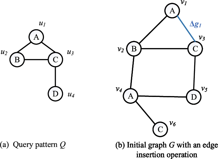Given an initial graph G, a graph update stream Δg consisting of edge insertions and deletions and a query graph Q. Then the continuous subgraph matching problem is to report positive (resp. negative) matches for each edge insertion (resp. deletion) operation.

Example 1.

Figure 1 shows an example of continuous subgraph matching. Given a query pattern Q as show in Fig. 1(a), and an initial graph G with an edge insertion operation Δg1 as show in Fig. 1(b), it is necessary to find all positive matches for each operation. When Δg1 occurs, it report a positive match {v1,v2,v3,v5}.

Fig. 1.

An example of continuous subgraph matching.

However, these applications deal with dynamic graphs in such a setup that is often essential to be able to support hundreds or thousands of continuous queries simultaneously. Optimizing and answering each query separately over the dynamic graph is not always the most efficient. Zervakis et al. [30] first propose a continuous multi-query process engine, namely, TRIC, on the dynamic graph. It decomposes the query graphs into minimum covering paths and constructs an index. Whenever an update occurs, it continuously evaluates queries by leveraging on the shared restrictions present in query sets. Although TRIC can achieve a better performance than a-query-at-a-time approaches, it still has some serious performance problems. (1) TRIC needs to maintain a large number of materialized views, leading to worse performance in storage cost. (2) Since TRIC decomposes each query graph Q in the queries set into a set of path conjuncts, and it will cause inevitably expensive join and exploration cost for the large sets of query paths; and (3) TRIC has an expensive maintenance cost of materialized results when updates occur on the graph.

These problems of existing methods motivated us to develop a novel concept of annotated query graph (AQG), which is obtained by merging all the queries into one. Similar to prior multi-query optimization approaches, our technique relies on sharing computation to speed up query processing. Each edge e in the AQG is annotated by the queries that contain e. In order to avoid executing subgraph pattern matching repeatedly whenever some edges expire or some new edges arrive, we need to construct an auxiliary data structure to record some intermediate query results. Note that data-centric representation of intermediate results is claimed to have the best performance in storage cost [15]. It maintains candidate query vertices for each data vertex using a graph structure such that a data vertex can appear at most once. In this paper, we also adopt this solution and construct a newly data-centric auxiliary data structure, namely, MDCG, based on the equivalent query tree of AQG. The purpose is to take advantage of the pruning power of all edges in AQG, and execute fast query evaluation by leveraging tree structure.

In summary, our contributions are:

– We propose an efficient continuous multi-query matching system, IncMQO, to resolve the problems of existing methods.
– We define annotated query graph, in which corresponding matching results can be obtained in one pass instead of multiple.
– We construct a newly data-centric auxiliary data structure based on the equivalent query tree of the annotated query graph to represent the partial solution in a compact form.
– We propose an incremental maintenance strategy to efficiently maintain the intermediate results in MDCG for each update and quickly detect the affected queries. Then we propose an efficient matching order for the annotated query to conduct subgraph pattern matching.

We experimentally evaluate the proposed solution using three different datasets, and compare the performance against the three baselines. The experiment results show that our solution can achieve up to two orders of magnitude improvement in query processing time against the sequential processing strategy.

2.Preliminaries and framework

In this section, we first introduce several essential notions and formalize the continuous multi-query processing over dynamic graphs problem. Then, we overview the proposed solution.

2.1.Preliminaries

We focus on a labeled undirected graph G=(V,E,L). Here, V is the set of vertices, E⊂V×V is the set of edges, and L is a labeling function that assigns a label l to each v∈V. Note that our techniques can be readily extended to handle directed graphs.

Definition 1

Definition 1(Graph Update Stream).

A graph update stream Δg is a sequence of update operations (Δg1,Δg2,…), where Δg1 is a triple ⟨op,vi,vj⟩ such that op={I,D} is the type of operations, with I and D representing edge insertion and deletion of an edge ⟨vi,vj⟩.

A dynamic graph abstracts an initial graph G and an update stream Δg. G transforms to G′ after applying Δg to G. Note that insertion of a vertex can be represented by a set of edge insertions; similarly, deletion of a vertex can be considered as a set of edge deletions.

Definition 2

Definition 2(Subgraph homomorphism).

Given a query graph Q=(VQ,EQ,LQ), a data graph G=(VG,EG,LG), Q is homomorphic to a subgraph of G if there is a mapping (or a match) f between them such that: (1) ∀v∈VQ, LQ(v)=LG(f(v)); and (2) ∀(vi,vj)∈EQ, (f(vi),f(vj))∈EG, where f(v) is the vertex in G to which v is mapped.

Since subgraph isomorphism can be obtained by just checking the injective constraint [15], we use the subgraph homomorphism as our default matching semantics. Note that we omit edge labels for ease of explanation, while the actual implementation of our solution and our experiments support edge labels.

Based on the above definitions, let us now define the problem of multi-query processing over dynamic graphs.

Problem statement Given a set of query graphs QDB={Q1,Q2,…,Qn}, an initial data graph G and graph update stream Δg, the problem of continuous multi-query processing over dynamic graph consists of continuously calculating positive or negative matching results for each affected query graphs Qi∈QDB when applying incoming updates.

2.2.Overview of solution

In this subsection, we overview the proposed solution, which is referred to as IncMQO. Specially, we are to address two technical challenges:

– Representation of intermediate results should be compact and can be used to calculate the corresponding matches of affected queries in one pass.
– Update operation needs to be efficient such that the intermediate results can be maintained incrementally to quickly detect the affected queries.

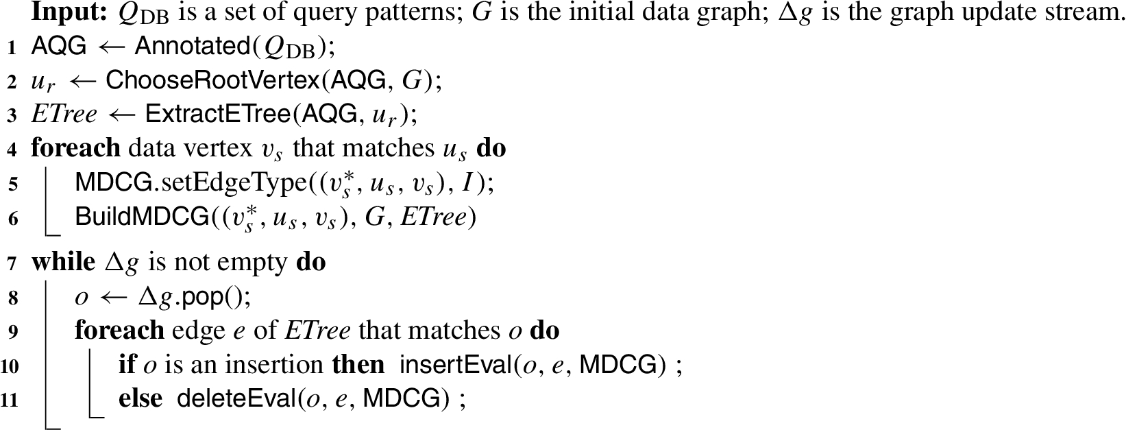
The former challenge corresponds to Continuous Multi-query Processing Model, while the latter corresponds to Continuous Multi-Query Evaluation Phase.

Algorithm 1 shows the outline of IncMQO, which takes an initial data graph G, a graph update stream Δg and queries set QDB as input, and find the matching results of affected queries when necessary. We first merge all the queries in QDB into an annotated query graph (AQG) (Line 1). Then, we extract from the annotated query graph AQG a equivalent query tree ETree by choosing a root vertex ur (Lines 2–3). The purpose is to take advantage of the pruning power of all edges in AQG, and execute fast query evaluation by leveraging tree structure. Based on ETree, we construct an auxiliary data structure from each start vertex us in the ETree (see Section 3), namely, MDCG, which is able to provide guidance to get affected queries and generate corresponding matches with light computation overhead (Line 4–6), here v∗ is a virtual vertex that conveniently represents the parent vertex of the root vertex. Finally, we perform continuous multi-query matching for each update operation. During a graph update stream, when an update comes, we first check whether it is an update that can affect the query results, i.e., check whether an edge e of ETree matches the corresponding edge in the operation o. If so, we amend the auxiliary data structure MDCG depending on the update type of the operation o, and calculate the positive or negative matching results for affected queries if necessary (Lines 7–11).

Algorithm 1:

IncMQO

3.Continuous multi-query processing model

When an edge update occurs, it is costly to conduct sequential query processing. The central idea of multi-query handling is to employ a delicate data structure, which can be used to compute matches of affected queries in one pass.

3.1.Annotated query graph

Different from the work proposed in [30] that decomposes queries into covering paths and handles updates by finding affected paths, we provide a novel concept of annotated query graph, namely, AQG, which merges all queries in QDB into one. An AQG is a pair (QA,δ), where QA is the merged query and δ is a function that annotates each edge e∈QA with a set δ(e) of query IDs from QDB. Intuitively, for each Q′∈δ(e), δ(e) indicates that e is an edge in query Q′, i.e., δ(e) is a condition on whether e is an edge in Q′. To construct AQG, for each graph Qi∈QDB, we first add a subscript to each vertex label in Qi to distinguish the vertices that have the same labels. That is, we randomly use {0,1,…,n} as subscripts for the n duplicate vertex labels in each query Qi. Then, for each unvisited edge e in Qi, we check whether it exists in other queries {Q′}. If so, we add {Q′} into δ(e) and mark e and corresponding edges in other queries as visited. We repeat this process till all the edges of each query in QDB have been visited. Finally, we construct AQG by merging {e} and {δ(e)} together. Based on AQG, we can compute matches of affected queries in one pass of enumeration instead of multiple.

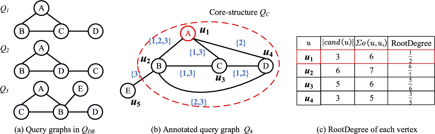
Example 2.

The queries in Fig. 2(a) are overlaped and can be merged into an annotated AQG (Q4,δ), where AQG (Q4,δ) takes the union of the vertices and edges of the three query graphs. The edges in (Q4,δ) are annotated by δ such that δ(u1,u2)={1,2,3}, δ(u1,u3)=δ(u2,u3)={1,3}, δ(u1,u4)={2}, δ(u2,u4)={2,3}, δ(u2,u5)={2,3}, δ(u3,u4)={1,2} (labels omitted here). Observe that common sub-patterns of Q1−Q3 are represented only once in Q4 and the matches to Q1−Q3 can be computed in a single enumeration of matches of (Q4,δ).

Remark.

Note that, there exists a case that the queries in the QDB have no common component. In this condition, we will process each query in QDB sequentially. In Section 6.11, we evaluate the performance of single query processing against TurboFlux. The experiment results prove that our algorithm is still more efficient.

Fig. 2.

Annotated query graph.

3.2.Auxiliary data structure

Since continuous multi-query processing is triggered by each update operation on the data graph, it is more useful to maintain some intermediate results for each vertex in the data graph as TurboFlux [15] did rather than in the query graph. To this end, we propose a newly data-centric auxiliary data structure based on the equivalent query tree of AQG.

Definition 3.

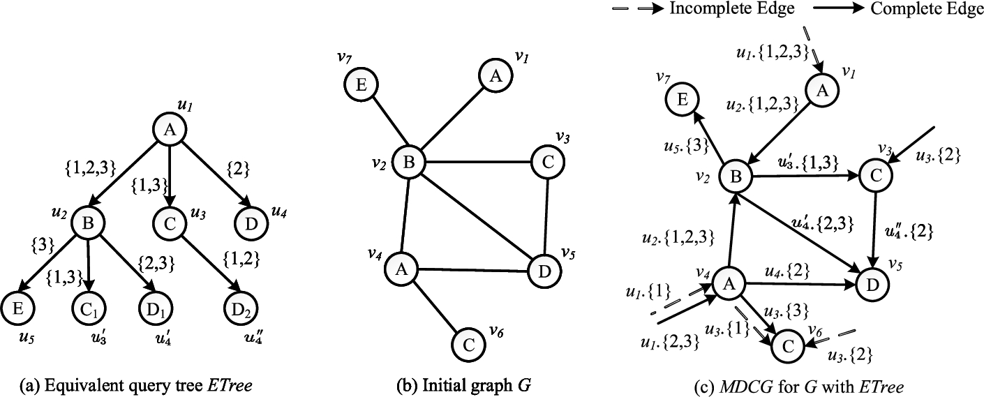
The equivalent query tree of a rooted AQG is defined as the tree ETree such that each edge in AQG corresponds to a tree edge in ETree. (e.g., Fig. 3(a) is the equivalent query tree of AQG Q4 in Fig. 2(b)).

Note that since we will transform all edges of AQG into tree edges, there are duplicate vertices in ETree (e.g., u3 and u3′ in Fig. 3(a)). To construct ETree, we need to choose a root vertex of AQG. We first adopt the core-forest decomposition strategy of [1] to determine the core part QC(VC,EC). Then, we use edge overlapping factor o(e) and candidates set cand(u) (u∈VC) to select the root vertex ur in VC. In detail, we quantify u′s root degree as |cand(u)|/∑o(u,ui) (u∈VC, (u,ui)∈EC) and select the vertex with the minimum value as the root vertex ur. Here, o(u,ui) is the overlapping factor of edge (u,ui), defined as the maximum number of queries annotated on edge (u,ui) in the AQG (e.g., o(u1,u2)=3 in Fig. 2(b)), and |cand(u)| represents a set of vertices in G matching with u. After that, we traverse AQG in a BFS order from ur, and direct all edges from upper levels to lower levels to generate the equivalent query tree of AQG.

Example 3.

For each vertex ui in AQG, supposed that the number of candidates (i.e., |cand(ui)|) is shown in Fig. 2(c). We select the vertex with the lowest root degree as root vertex (i.e., vertex u1) and then generate the equivalent query tree ETree as shown in Fig. 3(a).

Fig. 3.

Example of constructing MDCG.

Observation 1.

Let (ui,uj) be an edge in ETree. For each annotated query ID Qi on (ui,uj), there must exist a path from a vertex us to uj corresponding to Qi and us has no incoming edge annotated with Qi. Here, us is called start vertex.

Example 4.

Consider the edge (u3,u4″) in Fig. 3(a). The start vertex corresponding to Q1 and Q2 is u1 and u3, respectively.

Based on ETree and AQG, we construct a novel data-centric auxiliary data structure called MDCG. For each vertex v in the data graph, we store corresponding candidate query vertices as incoming edges to v in intermediate results. The MDCG is a complete multigraph such that every vertex pair (vi,vj) (vi,vj∈VG) has |VQA|−1 edges. Here, each edge has a query vertex ID in ETree as edge label, and its state is one of Null/Incomplete/Complete. Each query vertex ID contains an annotation set σ(u) about query ID that conform corresponding states. Let us be one start vertex of ETree and vs be one vertex in G to which us matches. Given an edge (v,u′,v′) with σ(u)={Qi,…,Qj} in the MDCG, it belongs to one of the following three types.

– Null edge: For each query Qk (k∈[i,j]), there is no data path vs→v.v′ that match us→P(u′).1 1u′.
– Incomplete edge: u′ is a candidate of v′ such that for each Qk (k∈[i,j]), (1) there exists a data path vs→v.v′ that match us→P(u′).u′; and (2) there exists a subtree of u′ does not match any subtree of v′.
– Complete edge: u′ is a candidate of v′ such that for each Qk (k∈[i,j]), (1) there exists a data path vs→v.v′ that match us→u.u′; and (2) every subtree of u′ matches the corresponding subtree of v′.

Note that we do not store Null edges in the MDCG since they are hypothetical edges in order to explain the incremental maintenance strategy (see Section 4). Furthermore, to reduce the storage cost, we use a bitmap for each vertex v in the MDCG where the i-th bit indicates whether v has any incoming Incomplete edges whose label is ui.

Example 5.

Figure 3(c) gives the MDCG based on ETree in Fig. 3(a). Since there is a path u1→u2.u4′ from start vertex u1 corresponding to Q2 and Q3 that matches v4→v2.v5 and u4′ does not have any subtree, then edge (v2,u4′,v5) with σ(u4′)={Q2,Q3} in the MDCG is set to be a Complete edge.

4.Continuous multi-query evaluation phase

We rely on an incremental maintain strategy to efficiently maintain MDCG for each edge update operation, and then propose an effective matching order to conduct subgraph pattern matching for affected queries in single pass of enumeration directly.

4.1.Incremental maintenance of intermediate results

We propose an edge state transition model to efficiently identify which update operation can affect the current intermediate results and/or contribute to positive/negative matches for each affected query. The edge state transition model consists of three states and six transition rules, which demonstrates how one state is transited to another.

Fig. 4.

Maintenance strategy.

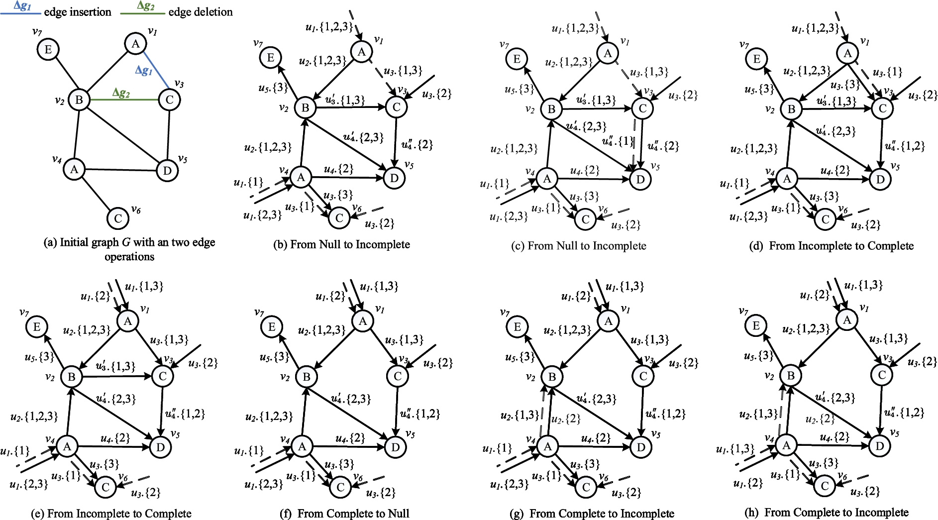
Handing edge insertion When an edge insertion (v,v′) occurs, we have the following three edge transition rules.

From Null to Null. (1) Suppose that edge (v,v′) fails to match any query edge in the ETree, then the state of (v,v′) is Null. (2) Suppose that edge (v,v′) matches a query edge (u,u′) in the ETree. If v in the MDCG has no Incomplete/Complete incoming edge with label u such that σ(u) contains one query ID in δ(u,u′), then the state of (v,u′,v′) remains Null.

From Null to Incomplete. (1) Suppose that edge (v,v′) matches a query edge (u,u′) in the ETree. If v has an Incomplete/Complete edge (vp,v) with label u such that σ(u)∩δ(u,u′)=ζ (ζ≠∅), then we transit the state of edge (v,u′,v′) from Null to Incomplete and set σ(u′)=ζ. (2) Suppose that the state of edge (v,u′,v′) in the MDCG is translated from Null to Incomplete, we need to propagate the update downwards. That is, for each adjacent vertex v″ of v′, we will check whether (v′,v″) matches (u′,u″) where u″ is the child vertex of u′ and σ(u′)∩δ(u′,u″)=ζ′ (ζ′≠∅). If so, we transit the state of (v′,u″,v″) in the MDCG from Null to Incomplete and set σ(u″)=ζ′.

Example 6.

Figure 4(b)–(c) give the example of edge transition rule from Null to Incomplete. In Fig. 4(a), when the edge insertion operation Δg1 (between v1 and v3) occurs, we can find that (v1,v3) matches (u1,u3) in the ETree. Since v1 has an incoming Incomplete edge with label u1 such that σ(u1)∩δ(u1,u3)={1,3} in Fig. 4(b), then we translate the state of edge (v1,u3,v3) from Null to Incomplete and set σ(u3)={1,3}. Next, update needs to be propagated downwards. Here, an Incomplete edge (v3,u4″,v5) with σ(u4″)={1} is added into the MDCG, as shown in Fig. 4(c).

From Incomplete to Complete. (1) Suppose that the state of (v,u′,v′) is transited from Null to Incomplete. If u′ is a leaf vertex in the ETree for a query Qi in σ(u′), we transit the state of (v,u′,v′) with σ(u′)={Qi} in the MDCG from Incomplete to Complete. The state of edge (v,u′,v′) with σ(u′)/({Qi}) remains Incomplete. (2) Suppose that the state of (v,u′,v′) in the MDCG is transited from Incomplete to Complete. If v has an outgoing Complete edge in the MDCG whose label is u″ and σ(u″) contains Qi for every u″ in Children(P(u′)), then transit the state of every Incomplete incoming edge (vp,v) of v in the MDCG whose label is P(u′) and σ(P(u′)) contains Qi from Incomplete to Complete. The state of edge (vp,P(u′),v) with σ(P(u′))/({Qi}) remains Incomplete.

Example 7.

Figure 4(d)–(e) give the example of edge transition rule from Incomplete to Complete. In Fig. 4(d), since u3 is the leaf vertex in Q3, the state of edge (v1,u3,v3) with σ(u3)={3} is transited from Incomplete to Complete. Currently, the state of edge (v3,u4″,v5) with σ(u4″)={1} in Fig. 4(c) is transited from Null to Incomplete. Since u4″ is the leaf vertex of Q1, then the state of edge (v3,u4″,v5) with σ(u4″)={1} is transited from Incomplete to Complete. Note that there is another Complete edge (v3,u4″,v5) with σ(u4″)={2}, we can merge them together. Then, we further check the state of edge (v1,u3,v3) with σ(u3)={1}. Since v3 has an outgoing Complete edge with label u4″ and σ(u4″)={1} for every children of u3, then the state of edge (v1,u3,v3) with σ(u3)={1} is transited from Incomplete to Complete. Next, update needs to be propagated upwards. Here, the state of edge (v∗,u1,v1) with σ(u1)={1,3} is transited from Incomplete to Complete, as shown in Fig. 4(e).

Handing edge deletion When an edge deletion (v,v′) occurs, we have the following three reversed edge transition rules.

From Complete to Null. (1) For each edge (u,u′) in ETree such that v in the MDCG has an incoming Incomplete or Complete edge whose edge label is u, if (v,v′) matches (u,u′) and the state of (v,u′,v′) in the MDCG is Complete, then transit the state of (v,u′,v′) in the MDCG from Complete to Null. (2) Suppose that the state of edge (v,u′,v′) in the MDCG is transited from Incomplete or Complete to Null. For each query Qi in σ(u′), if v′ in the MDCG no longer has any incoming edge whose label is u′ that contains the annotation Qi, then for each u″ in Children(u′), transit the state of every outgoing Complete edge of v′ in the MDCG whose label is u″ that contain Qi from Complete to Null.

Example 8.

Figure 4(f) gives the example of edge transition rule from Complete to Null. In Fig. 4(a), when the edge deletion operation Δg2 (between v2 and v3) occurs, the state of edge (v2,u3′,v3) is translated from Complete to Null in the MDCG as show in Fig. 4(f), since v2 has an incoming Complete edge with label u2 and (v2,v3) matches (u2,u3′) in the ETree.

From Complete to Incomplete. Suppose that the state of (v,u′,v′) in the MDCG is transited from Complete to Incomplete or Null. For each query Qi in σ(u′), if v in the MDCG no longer has any outgoing Complete edge whose label is u′ that contains Qi, then we transit the state of every incoming Complete edge of v in the MDCG whose label is P(u′) that contains Qi from Complete to Incomplete.

Example 9.

Figure 4(g)–(h) give the example of edge transition rule from Complete to Incomplete. In Fig. 4(g), since the state of edge (v2,u3,v3) is translated from Complete to Null, for Q1 and Q3, v2 does not have an outgoing Complete edge for every children of u2 in ETree, then the state of edge (v4,u2,v2) with σ(u2)={1,3} is transited from Complete to Incomplete. While the state of edge (v4,u2,v2) with σ(u2)={2} is still remained Complete, since it meets the Complete requirement for Q2. Next, update needs to be propagated upwards. Here, the state of edge (v∗,u1,v4) with σ(u1)={3} is transited from Complete to Incomplete, as shown in Fig. 4(h).

From Incomplete to Null. (1) If v in the MDCG has an incoming Incomplete or Complete edge whose edge label is u, and the state of (v,u′,v′) in the MDCG is Incomplete, then transit the state of (v,u′,v′) in the MDCG from Incomplete to Null. (2) Suppose that the state of (v,u′,v′) in the MDCG is transited from Incomplete or Complete to Null. For each query Qi in σ(u′), if v′ in the MDCG no longer has any incoming edge whose label is u′ that contains Qi, then for each u″ in Children(u′), transit the state of every outgoing Incomplete edge of v′ in the MDCG whose label is u″ that contain Qi from Incomplete to Null.

4.2.Subgraph search phase

If the state of an edge (v,u′,v′) is translated to Complete, we say the queries in σ(u′) are affected queries caused by edge (v,v′). Then, we propose an efficient algorithm, namely, MMatchinc, to calculate corresponding positive matches including (v,v′) for each affected query based on the MDCG in single pass of enumeration directly. The main idea of MMatchinc is explained as follows: (1) We derive a matching order based on the number of affected queries on each edge in ETree; and then (2) compute the positive matches for each affected query based on the matching order.

In order to calculate the matching order, MMatchinc first marks u′ as visited. Subsequently, given a set of unvisited vertices that is adjacent to u′ in ETree, the next vertex u∗ is the one such that δ(u∗,u′) contains the maximal affected queries. If there is a tie, it chooses a query vertex having a minimum number of candidate data vertices in the MDCG. After that, we mark u∗ as visited. The matching order for the rest of query vertices is determined along the same lines.

Remark.

Intuitively, MMatchinc outputs a “global” matching order for the query vertices in the AQG QA. It prioritizes vertices that are shared by more queries. Matching such vertices at an early stage could help avoid the enumeration of many unpromising intermediate results since the corresponding pruning benefits multiple queries at the same time.

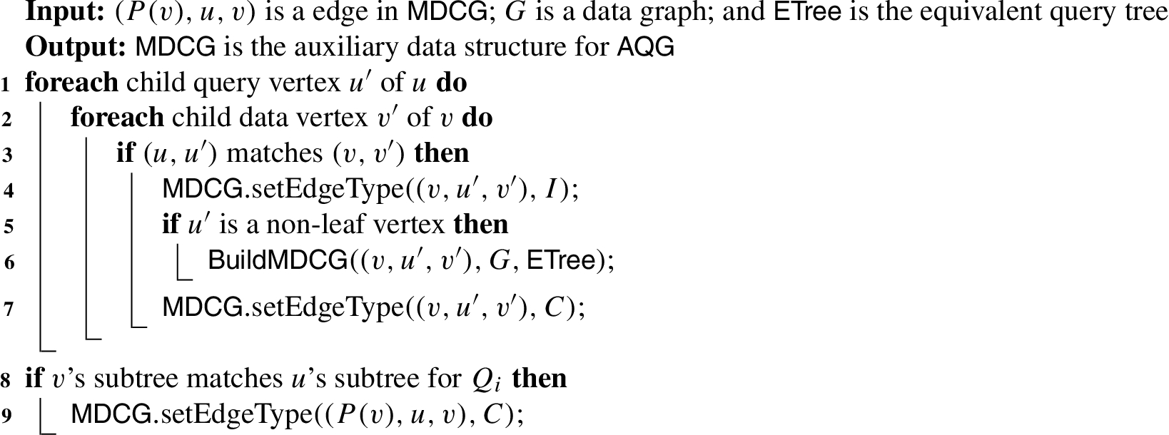
In the next stage, MMatchinc enumerates the positive matches for each affected query graph Qi embedded in the MDCG following the proposed matching order. It adopts the generic backtracking approach. During the matching process, it enumerates and prunes v′ adjacent Complete edge by inspecting edge label whether it contains the affected query Qi. The same edge for different query graphs is indeed enumerated only once.

Algorithm 2:

BuildMDCG

Example 10.

As show in Fig. 3(d), the state of edge insertion (v1,u3,v3) is translated into Complete. Since σ(u3)={1,3}, then Q1 and Q3 are the affected query graphs. Firstly, we mark u3 as visited. Then, for each adjacent vertex (i.e., u1 and u4″) in the ETree (see Fig. 2(a)), we choose u1 as the next vertex for matching since δ(u1,u3) contains both Q1 and Q3. Finally, a matching order {u3,u1,u2,u3′,u5,u4,u4′,u4″} is deduced. Based on the matching order, MMatchinc enumerates all the positive matches of the affected query graphs in a single pass.

5.IncMQO algorithms

In this section, we present detailed algorithms for IncMQO. In order to efficiently handle the continuous multi-query, we first construct the auxiliary data structure MDCG, and then present two major functions insertEval and deleteEval to apply necessary transition rules to efficiently maintain the intermediate results for each update. Finally, we investigate the matching algorithm MMatchinc to report corresponding positive/negative matches in one pass based on the MDCG.

5.1.MDCG construction

In this subsection, we explain BuildMDCG (Line 6 of Algorithm 1) which is designed for every v with an Incomplete incoming edge. It uses a depth-first travel strategy to extend each v in MDCG. First, we check whether there exists an edge (u,u′) matching (v,v′), where u′ and v′ represent a child vertex of u and v, respectively; if so, we transit the type of edge (v,u′,v′) from Null to Incomplete (Line 1–4). If u′ is not a leaf vertex, we call BuildMDCG recursively to match the child vertex of u′ (Lines 5–6). Otherwise, transit the state of the edge (v,u′,v′) from Incomplete to Complete (Line 8). After that, we check if the subtree of v matches the corresponding subtree of u for Qi; if so, we transit the state of the edge (p(v),u,v) from Incomplete to Complete (Lines 8–9).

Lemma 1.

The time complexity of BuildMDCG is O(|E(G)|∗|V(ETree)|).

Proof.

In the worst case, BuildMDCG is called for every vertex u and every data vertex v. Thus, given u and v the time complexity for Lines 1–2 of Algorithm 2 is O(|children(v)|∗|children(u)|). Note that the time complexity for Lines 8–9 is O(children(u)). Thus, the time complexity of BuildMDCG is O(∑u∈ETree∑v∈G(|children(v)|∗|children(u)|))=O(|E(G)|∗|V(ETree)|) □

5.2.Edge insertion

insertEval (Algorithm 3) is invoked for each new arrival edge (v,v′). The main idea of insertEval is explained as follows: we try to match (v,v′) with the query edges in ETree and update the MDCG based on the corresponding maintenance strategy. Then we build the MDCG downwards for the subtree of v′ and further update the MDCG upwards until reaching any of the starting vertex vs. Finally, we execute the subgraph matching to report the matching results.

Algorithm 3:

insertEval

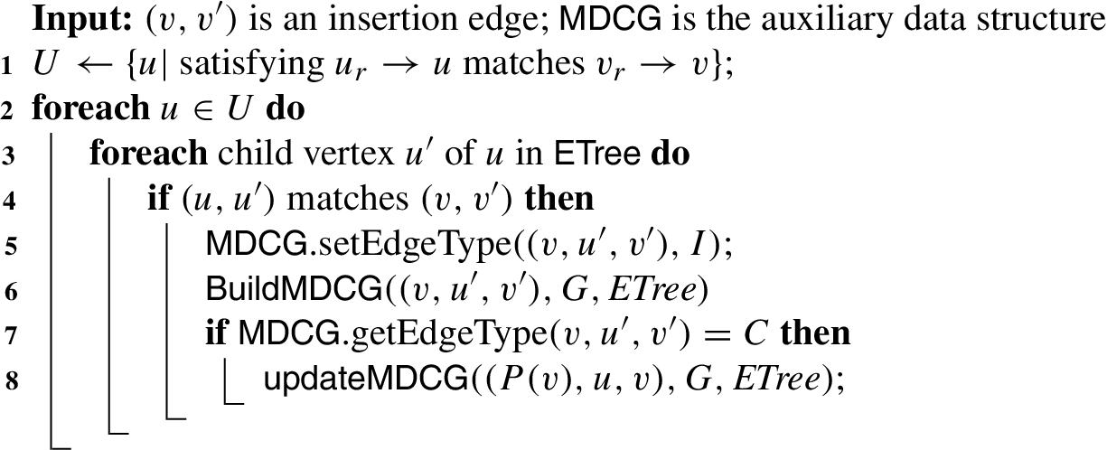
Note that not all the insertion edge (v,v′) can cause the update of MDCG. Only when there is a path vs→v matches the path us→u, the insertion operation can cause any update to MDCG. Thus we collect all the path matched vertex u into a vertex set U (Line 1). To do this, we can guarantee v has an Incomplete or Complete edge. Then for each child query vertex u′ of u (u∈U), if (u,u′) matches (v,v′), we further set the type of edge (v,u′,v′) to Incomplete with the transition rule From Null to Incomplete, and execute BuildMDCG downwards to build the new part of MDCG (Lines 2–6). If the type of the insertion edge (v,v′) transit into Complete finally, we execute updateMDCG to update the type of the edge which belongs to the path vs→v (Lines 7–8).

Algorithm 4:

updateMDCG

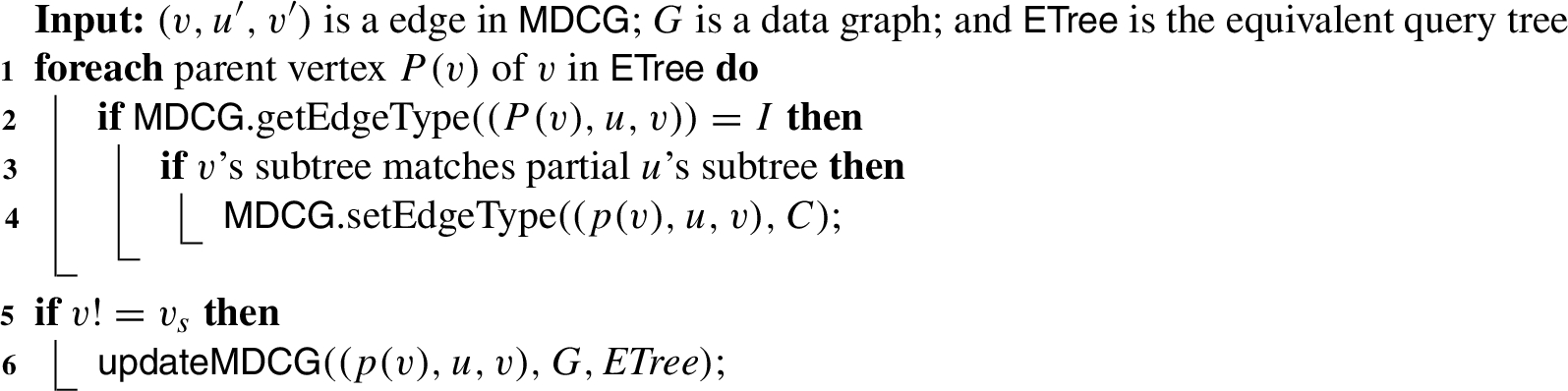
Here, updateMDCG (Algorithm 4) traverses the MDCG upwards and performs the transition rules if necessary. It is only called when v has an incoming edge with Incomplete type (Line 2). Then, when v’s subtree matches u’s subtree for Qi, we further transit (P(v),u,v)) to Complete with transit rule From Incomplete to Complete (Lines 3–4). When it reaches any starting data vertex vs, we end of the updateMDCG. On the contrary, we continue to recurse upwards(Lines 5–6).

Remark.

deleteEval algorithms for edge deletion are very similar to those for edge insertion except that they use different transition rules. Thus, we do not describe here.

6.Experiments

In this section, we perform extensive experiments on both real and synthetic datasets to show the performance of IncMQO algorithm for continuous multi-query matching over dynamic graphs. The performance of IncMQO was evaluated using various parameters such as the overlapped rate of query set, average query size, query database size, edge update size, and graph size. The proposed algorithms were implemented using C++, running on a Linux machine with two Core Intel Xeon CPU 2.2 Ghz and 32 GB main memory.

6.1.Datasets and query generation

The SNB dataset. SNB [5] is a synthetic benchmark designed to accurately simulate the evolution of a social network through time. This evolution is modeled using activities that occur inside a social network. Based on the SNB generator, we derived 3 datasets: (1) SNB0.1M with a graph size of |EG|=0.1M edges and |VG|=57K vertices; (2) SNB1M with a graph size of |EG|=1M edges and |VG|=463K; and (3) SNB10M with a graph size of |EG|=10M edges and |VG|=3.5M, and use the second one as default.

The NYC dataset. NYC2 2 is a real world set of taxi rides performed in New York City (TAXI) in 2013. TAXI contains more that 160M entries of taxi rides with information about the license, pickup and drop-off location, the trip distance, the date and duration of the trip, and the fare. We utilized the available data to generate a data graph with |EG|=1M edges and |VG|=280K vertices.

The BioGRID dataset. BioGRID [27] is a real world dataset that represents protein to protein interactions. We used BioGRID to generate a stream of updates that result in a graph with |EG|=1M edges and |VG|=63K vertices.

In order to construct the set of query graph patterns QDB, we identified two typical distinct query classes: trees and graphs. Each type of query graph pattern was chosen equiprobably during the generation of the query set. The default values for the query set are: (1) an average size l of 5, where l represents the average size of the queries in QDB; (2) a query database QDB size of 500 query graphs; and (3) a factor that denotes the percentage of overlap between the queries in QDB, θ=50%.

6.2.Comparative evaluation

Our method, denoted as IncMQO, is compared with a number of related works. TRIC is the state-of-the-art continuous multi-query processing method over dynamic graph [30]. It utilizes the common parts of minimum covering paths to amortize the costs of processing and answering them. TurboFlux [15] and GraphFlow [13] are the state-of-the-art continuous subgraph matching methods for single query. Both of them can be utilized for multi-query processing scenarios. That is, we adopt the sequential query processing strategy on them.

We measure and evaluate (1) the elapsed time and the size of intermediate results for IncMQO and its competitors by varying the percentage of overlap between the queries in the query set; (2) the elapsed time and the size of intermediate results for IncMQO and its competitors by varying the average query size and query database size; (3) the elapsed time and the size of intermediate results for IncMQO and its competitors by varying the edge insertion size; (4) the elapsed time and the size of intermediate results for IncMQO and its competitors by varying the edge deletion size; and (5) the scalability of IncMQO.

6.3.Evaluating the efficiency of IncMQO

In this subsection, we evaluated the performance of IncMQO against its competitors from the aspect of processing time and storage cost on three datasets: SNB1M, NYC and BioGRID with a default updates stream |Δg|=15%|G|.

Time efficiency comparison Fig. 5(1) shows the total processing time of IncMQO and its competitors over different datasets. We can see that IncMQO is better than its competitors over all datasets. Notably, IncMQO outperforms TRIC, TurboFlux and GraphFlow by up to 8.43 times, 28.93 times, and 385.21 times, respectively. The reason is that TRIC needs to maintain a large number of indexes to track the matching results; TurboFlux and GraphFlow need to process the multiple queries sequentially, which costs a lot of time overhead. In specific, GraphFlow has the worst performance, since it does not store any intermediate results and use the re-computing method for each update.

Space efficiency comparison Fig. 5(2) shows the size of intermediate results on each dataset. We only evaluate the IncMQO, TRIC, and TurboFlux, since GraphFlow does not maintain any intermediate results. IncMQO outperforms TRIC, and TurboFlux by up to 9.03 times, 29.07 times, respectively. This is because TRIC maintains a large number of materialized views and TurboFlux needs to construct auxiliary data structure for each query in the query set, as a result, leading to worse performance in storage cost.

Fig. 5.

Performance on SNB1M, NYC and BioGRID.

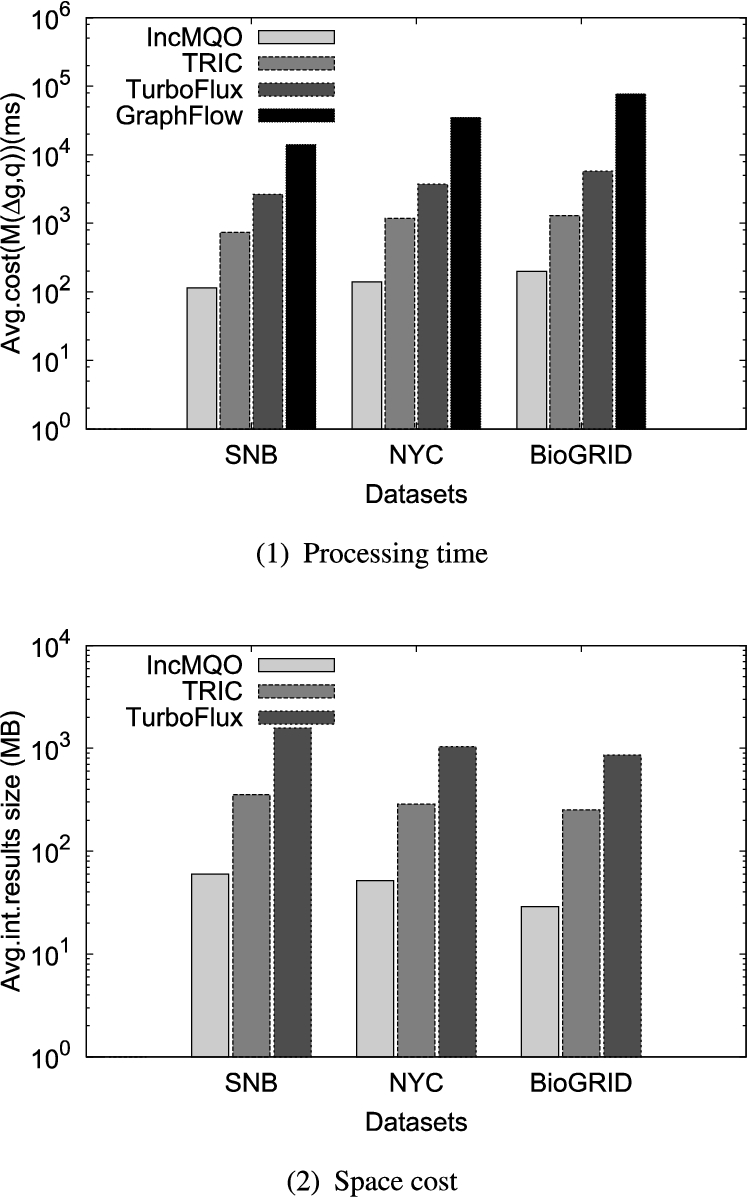
Fig. 6.

Performance of varying the percentage of query overlap.

6.4.Varying percentage of query overlap

In Fig. 6(1) we give the results of the time efficiency evaluation when varying the parameter θ, for 0%, 10%, 20%, 30%, 40%, 50% and 60% of a query set for |QDB|=500 on SNB1M dataset. Here, we fixed |Δg|=15%|G|. In this setup, the algorithms are evaluated for varying percentage of query overlap. θ=0% means that the queries in QDB have no overlap. It is revealed that IncMQO significantly outperforms other approaches when θ=0%. A higher number of query overlap should decrease the number of calculations performed by algorithms designed to exploit commonalities among the query set. The results show that IncMQO and TRIC behave in a similar manner as previously described, while TurboFlux and GraphFlow do not since they focus on a-query-at-a-time. Note that in Fig. 6(1), when θ=0%, IncMQO is slightly worse than that of TurboFlux while still better than that of TRIC by 1.25 times and GraphFlow by 5.07 times. Figure 6(2) plots the average size of intermediate results. IncMQO achieves the smallest size of intermediate results since it merges all the queries into one and builds a concise auxiliary data structure. In specific, IncMQO is superior to up to TurboFlux 63.2 times when θ=60%.

Fig. 7.

Performance of varying the average query size.

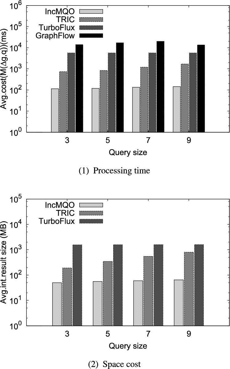
6.5.Varying the average query size

In this subsection, we evaluate the impact of the average query size in QDB on the performance of IncMQO and its competitors. Figure 7(1)–(2) show the performance results on SNB1M dataset. We set l from 3 to 9 in 2 increments and fixed |Δg|=15%|G|. Note that the matching cost does not always increase as the average query size increases. Figure 7(1) shows the elapsed time, IncMQO significantly outperforms its competitors regardless of average query size. Specially, IncMQO outperforms TRIC by 6.40–11.72 times, TurboFlux by 39.06–49.24 times and GraphFlow by 139.90–172.33 times. Figure 7(2) gives the average size of intermediate results. It is reviewed that the average size of intermediate result of TRIC increases rapidly with the increase of the average query size. In specific, IncMQO outperforms TRIC by up to 12.31 times when l is 9. Since TRIC uses path join operations, the larger the query graph pattern, the more join operations it requires.

Fig. 8.

Performance of varying query database size.

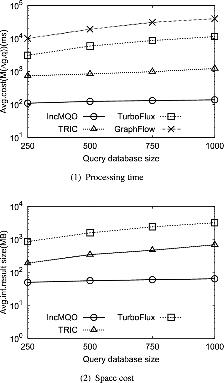
6.6.Varying query database size

In this subsection, we evaluate the impact of the size of query database on the performance of IncMQO and its competitors. Figure 8(1)–(2) show the performance results using SNB for varying the size of the query database QDB. More specifically, we fix |Δg|=15%|G| and vary |QDB| from 250 to 1000 in 250 increments. Please notice the y-axis is in a logarithmic scale. Figure 8(1) shows the processing time for each algorithm when varying |QDB|. It revealed that IncMQO significantly outperforms its competitors regardless of query database size. Specially, IncMQO outperforms TRIC by up to 8.92 times, TurboFlux by up to 82.73 times and GraphFlow by up to 287.77 times when |QDB|=1000. IncMQO also outperforms its competitors in terms of the size of intermediate results, as shown in Fig. 8(2). The performance gap between IncMQO and TRIC will increase as |QDB| increases. Specially, the average size of intermediate results of TRIC and TurboFlux is larger than that of IncMQO by up to 10.78 times and 50.47 times, respectively, when |QDB|=1000.

Fig. 9.

Performance of varying the edge insertion size.

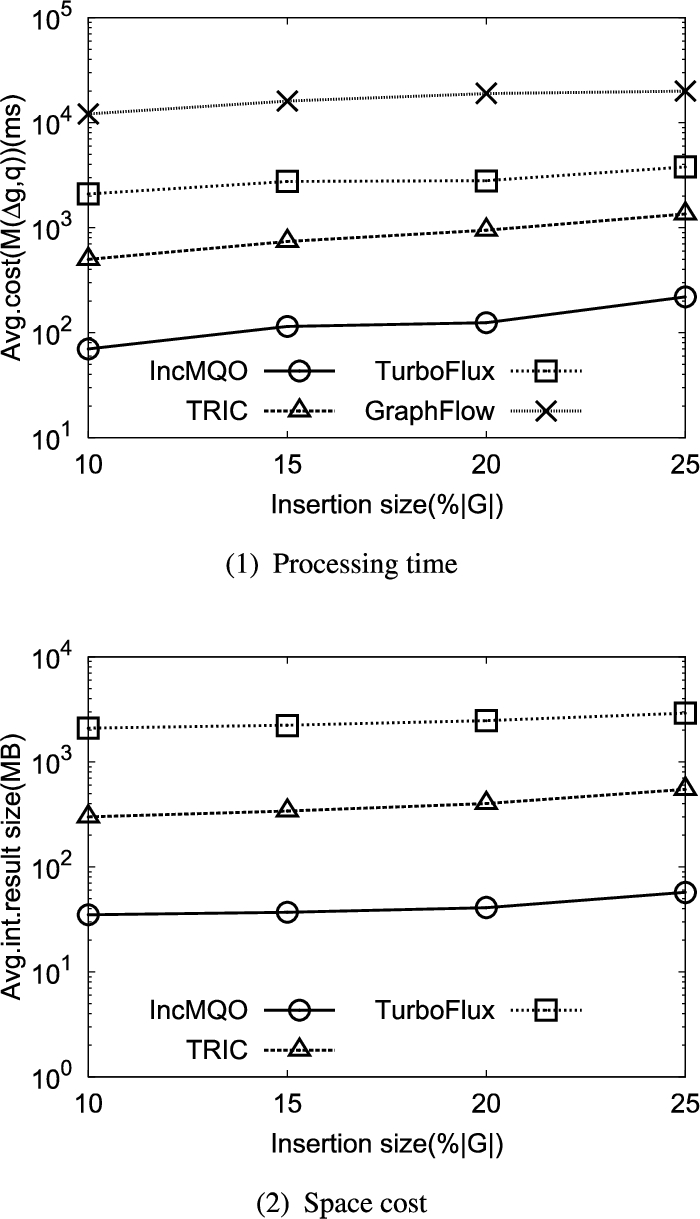
6.7.Varying the edge insertion size

Figure 9(1)–(2) show the performance results using SNB1M for varying edge insertion size. Here, we vary the number of newly-inserted edges from 10%|G| to 25%|G| in 5%|G| increments with respect to the number of triples in the graph update stream. Figure 9(1) shows the total processing time for each algorithm. The results demonstrate that all algorithm’s behavior is aligned with our previous observations. It can be seen that IncMQO has consistent better performance than its competitors. Specially, IncMQO outperforms TRIC by up to 6.43 times, TurboFlux by up to 24.04 times and GraphFlow by up to 152.33 times. In terms of the size of intermediate results, IncMQO also has a better performance than its competitors, as shown in Fig. 9(2). Specially, the average size of intermediate results of TRIC and TurboFlux is larger than that of IncMQO by up to 9.96 times and 60.24 times, respectively, when the insertion size is 20%|G|.

Fig. 10.

Performance of varying the edge deletion size.

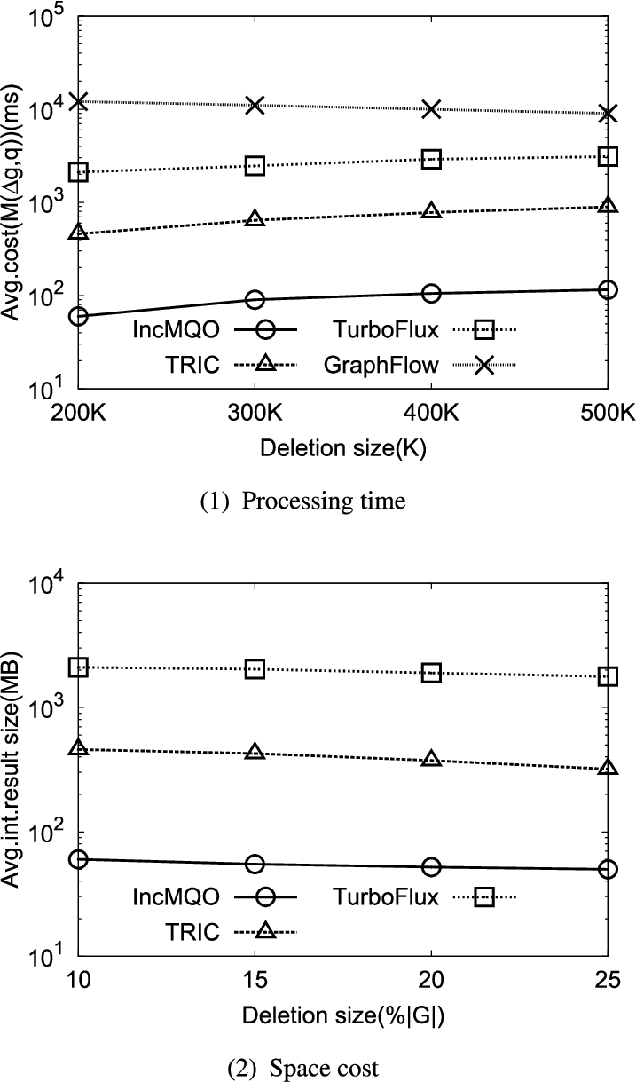
6.8.Varying the edge deletion size

Figure 10(1)–(2) show the performance results using SNB1M for varying edge deletion size. Here, we vary the number of expired edges from 10%|G| to 25%|G| in 5%|G| increments with respect to the number of triples in the graph update stream. Figure 10(1) shows the total processing time for each algorithm. Note that deletion of an edge (v,v′) may affect the auxiliary data structure. As the edge deletion size increases, incremental subgraph matching times of IncMQO, TRIC, and TurboFlux increase, while that of GraphFlow decreases. The reason is that the edge deletions reduce the input data size of GraphFlow directly. Nevertheless, IncMQO still consistently outperforms its competitors regardless of the edge deletion size. As shown in Fig. 10(2), the average number of intermediate results of TRIC is larger than that of IncMQO by up to 6.4 times, and TurboFlux is larger than that of IncMQO by up to 23.4 times when the deletion size is 20%|G|.

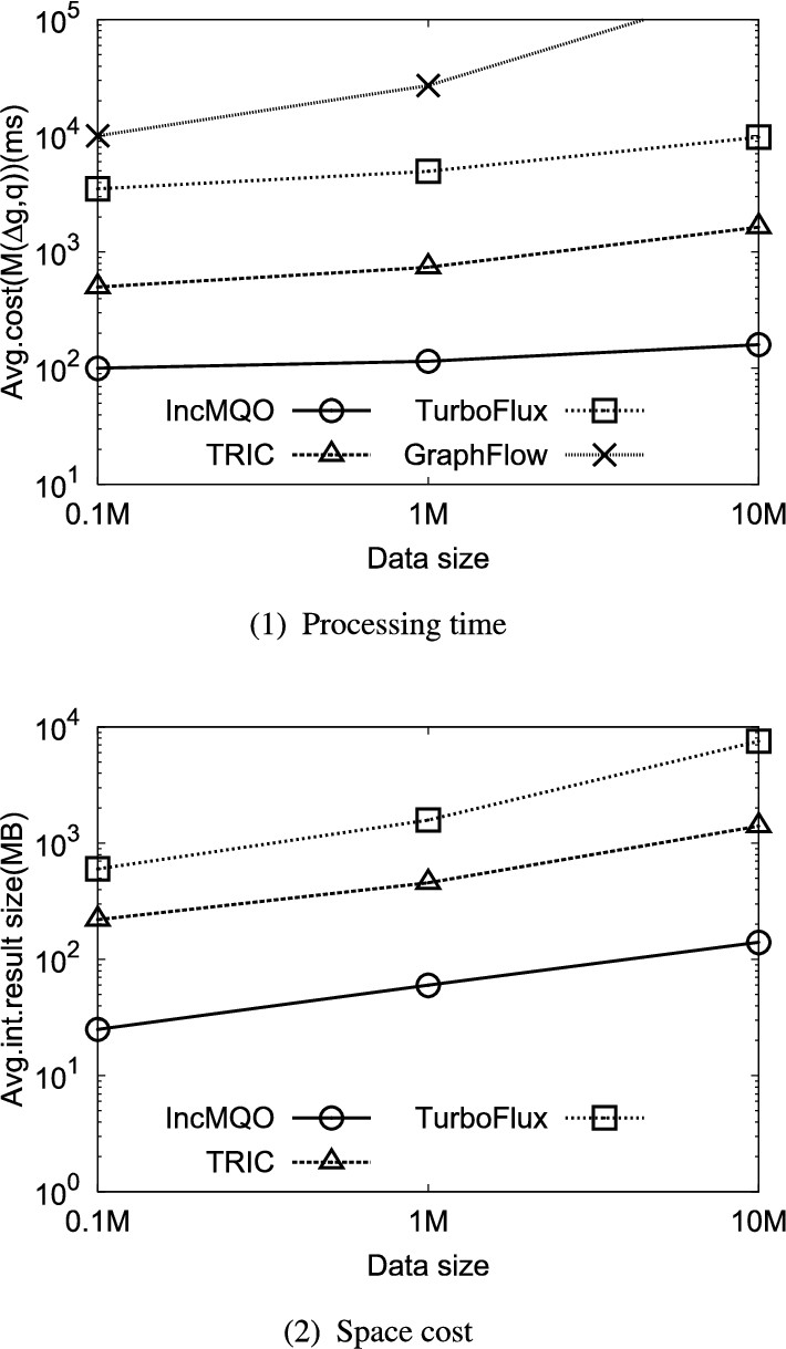
6.9.Varying dataset size

Figure 11(1)–(2) show the performance results using SNB for varying dataset size. Here, we fixed |Δg|=15%|G| and varied the size of SNB from 0.1M to 10M. In Fig. 11(1), IncMQO consistently outperforms its competitors regardless of the dataset size. In specific, the figure reads a non-exponential increase as the dataset size grows. The scalability suggests that IncMQO can handle reasonably large real-life graphs as those existing algorithms for deterministic graphs. Figure 11(2) shows similar scalability of intermediate result sizes for IncMQO, TRIC and TurboFlux. Specially, IncMQO outperforms TRIC by up to 10.70 times and TurboFlux by up to 53.86 times.

Fig. 11.

Performance of varying dataset size.

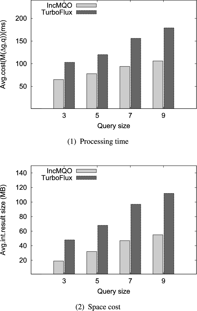
6.10.Comparison of different matching orders

In this set of experiments, we evaluate the performance of different matching orderings on SNB1M dataset. We compare our proposed matching order with that proposed in IncMQOTurbo. IncMQOTurbo adopts the subgraph matching algorithm of TurboFlux which used the candidate set of each query path to determine the matching order. We set l from 3 to 9 in 2 increments and fixed |Δg|=15%|G|. The results are within expectation. Figure 12(1) shows the elapsed time, IncMQO outperforms IncMQOTurbo by 1.91–2.76 times. Figure 12(2) gives the average size of intermediate results. IncMQO still performs better than IncMQOTurbo. Since IncMQO preferentially matches the vertices that are shared by more query which could help avoid the enumeration of many unpromising intermediate results.

Fig. 12.

Comparison of different matching orders.

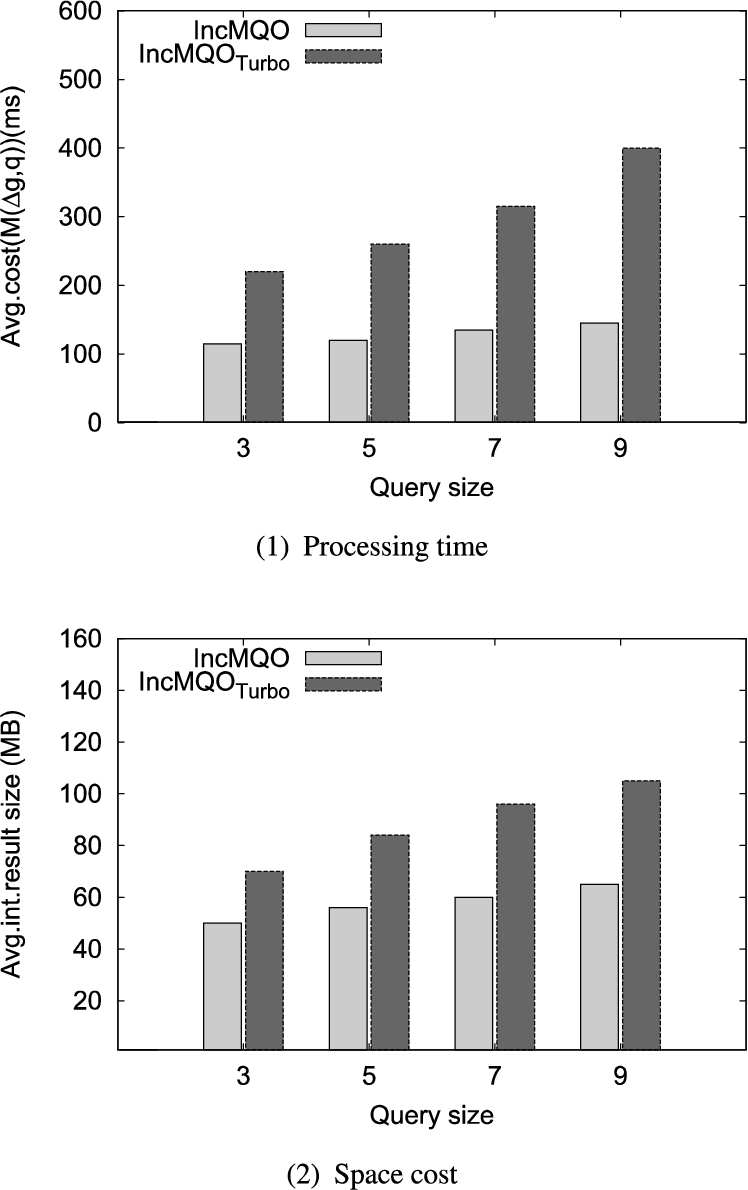
6.11.Performance evaluation of single query

In this set of experiments, we evaluate the performance of single query to text the efficiency when there is no common components in the query set QDB. Figure 13(1)–(2) show the performance results using SNB1M dataset between IncMQO (without AQG) and TurboFlux. We set l from 3 to 9 in 2 increments and fixed |Δg|=15%|G|. Specifically, IncMQO outperforms TurboFlux in terms of elapsed time and intermediate result size. This is because we translate the query graph into an equivalent query tree rather than a spanning tree. When there is a circle in the query graph, the spanning tree will ignore the non-tree edges, while the equivalent query tree takes both tree edges and non-tree edges into consideration. As a result, using an equivalent query tree can achieve a stronger pruning ability.

Fig. 13.

Performance evaluation of single query.

6.12.Comparison of incremental matching and recomputing algorithm

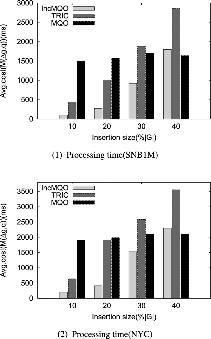
In this subsection, we further compare the incremental algorithm (IncMQO and TRIC) and the recomputing algorithm (MQO [23]) to detect the limitations that the number of updates brings to our algorithm. Recomputing algorithm means that conducts subgraph matching for pattern graph over updated data graph with batch mode. We conduct experiments on the two synthetic and real-life data graphs by varying the newly-inserted edges from 10%|G| to 40%|G| in 10%|G| increments with respect to the number of triples in the graph update stream. Figure 14(1) and Fig. 14(2) show the total processing time for each algorithm on SNB1M and NYC. We see that IncMQO behaves better than TRIC by 2.03–4.24 times and MQO by 1.34–14.30 times when the size of updates is no more than 30%|G|. However, when the number of edge insertion size continues to rise, the auxiliary data structure in the incremental matching needs to maintain a lot intermediate results, making it less effective than matching from scratch over the updated graph.

Fig. 14.

Results of the comparison.

7.Related work

We categorize the related work as follows.

Subgraph isomorphism research Subgraph isomorphism research is a fundamental requirement for graph databases and has been widely used in many fields. While this problem is NP-hard, in recent years, many algorithm have been proposed to solve it in a reasonable time for real datasets, such as VF2 [4], GraphQL [11], TurBOiSO [10], QuickSI [26]. Most all these algorithms follow the framework of Ullmann [28], with some pruning strategies, heuristic matching order algorithm and auxiliary neighborhood information to improve the performance of subgraph matching search. Lee et al. [17] compared these subgraph isomorphism algorithms in a common code base and gave in-depth analysis. However, these techniques are designed for static graphs and are not suitable for processing continuous graph queries on evolving graphs.

Multiple query optimization for relational database Multiple query optimization (MQO) has been well studied in relational databases [24,25]. Most work on relational database extend existing cost model based on statistics, and search for a global optimal access plan among all possible access plan combinations for each single query. Meanwhile, some intermediate access plan can be shared to accelerate multi-query evaluation. However, these relational MQO methods cannot be directly used for subgraph homomorphism search of MQO, because we do not assume that statistics or indexes exist on the data graph, and some relational optimization strategies (such as push selection and projection) are not suitable for subgraph homomorphism search. In addition, the methods of identifying common relation subexpression [7] are also difficult or inefficient for graph-based multi-query evaluation since it is inefficient to evaluate graph pattern queries by converting them into relational queries [11].

One-time multiple query evaluation Le et al. [16] studied the problem of evaluating SPARQL one-time multiple queries (SPARQL-MQO) over RDF graphs. Given a batch of graph queries, it clustered the graph queries into disjoint finer groups and then rewrote the patterns into a single query common pattern graph for each group. However, its clustering technique (and selectivity information) becomes degenerate and the construction of query sets ignores the cyclic structures in queries. Subsequently, Ren et al. [23] extended one-time multiple queries for an undirected labeled graph. It organized the useful common subgraphs and the original queries in a data structure called pattern containment map (PCM), and then it further cached the intermediate results based on PCM to balance memory usage and the execution time. Note that, PCM was designed for static graph. When using it in dynamic graph, we need reconstruct PCM for each update operation, which is practically infeasible. In contrast, our proposed MDCG stored intermediate results in the data graph for each data vertex which can reduce maintenance operations associated with data graph updates.

Continuous query process Continuous query process has first been considered in [29] which means continuously monitoring a set of graph streams and reporting the appearances of a set of pattern graphs in a set of graph streams at each timestamp [3,14]. But it offered an approximate answer instead of using subgraph isomorphism verification to find the exact query answers. In the latter study, Fan et al. [6] proposed the concept of incremental subgraph matching to handle continuous query problem. It only executed subgraph matching over the updated part, avoiding recomputing from scratch. In addition, Gillani et al. [9] proposed continuous graph pattern matching over knowledge graph streams and used two different executional models with an automata-based model to guide the searching process. Kim et al. [15] proposed a novel data-centric presentation to process continuous subgraph matching. However, all of the above algorithms evaluate each query separately and cannot be directly used for multi-query problem.

Continuous multiple query evaluation In addition, there are some researches on the topic of continuous multiple queries evaluation. Pugliese et al. [19] studied maintaining multiple subgraph query views under single-edge insertion workloads. It took advantage of common substructures and used an optimal merge strategy. However, it only focused on insertion. But in the real world, deletions also occur. Kankanamge et al. [12] studied the problem of optimizing and evaluating multiple subgraph queries continuously in a changing graph. It decomposed all the queries into multiple delta queries, which were then evaluated one query vertex at a time, without requiring any auxiliary data structures. Mhedhbi et al. [18] optimized both one-time and continuous subgraph queries using worst-case optimal joins. Since the methods in literatures [12] and [18] did not store any intermediate results, they needed to evaluate subgraph matching for each update, even if the update did not generate any positive/negative match. In recently, Zervakis et al. [30] handled the continuous multi-query problem over graph streams via decomposing the query into covering paths, and then it constructed a tree-based data structure to indexing and clustering continuous graph queries. However, this data structure is not concise enough, leading to many expensive join operations. Compared to covering paths, our proposed MDCG uses the data-centric representation of intermediate results, which is more concise. As a result, MDCG needs less memory consumption and has smaller maintenance costs for each update.

8.Conclusion and further work

In this paper, we proposed an efficient continuous multi-query processing engine, namely, IncMQO, in dynamic graphs. We showed that IncMQO can resolve the problems of existing methods and process continuous multiple subgraph matching for each update operation efficiently. We first developed a novel concept of annotated query graph that merges multi-query into one. Then we constructed a data-centric auxiliary data structure based on the equivalent query tree of the annotated query graph to represent partial solutions in a concise form. For each update, we proposed an edge transition strategy to maintain the intermediate results incrementally and detect the affected queries quickly. What’s more, we proposed an efficient matching order to calculate the positive or negative matching results for each affected query in one pass. Finally, comprehensive experiments performed on real and benchmark datasets demonstrate that our proposed algorithm outperforms alternatives.

A couple of issues need further study. We only simply consider the scenario that all the queries have been given at the start. However, the queries set will actually be updated due to users’ demands. To this end, we are going to consider this scenario in the future work and design an efficient algorithm to deal with the updates of queries set in multiple queries processing over dynamic graph.

Notes

1 P(u′) means the parent of u′ in ETree.

2 https://chriswhong.com/open-data/foil%20nyc%20taxi/

Acknowledgement

This work is partially supported by National key research and development program under Grant Nos. 2018YFB1800203, Tianjin Science and Technology Foundation under Grant No. 18ZXJMTG00290, National Natural Science Foundation of China under Grant No. 61872446, and National Natural Science Foundation of Hunan Province under grant No. 2019JJ20024.

References

[1]	F. Bi, L. Chang, X. Lin, L. Qin and W. Zhang, Efficient subgraph matching by postponing Cartesian products, in: Proceedings of the 2016 International Conference on Management of Data, ACM, San Francisco, CA, (2016) . doi:10.1145/2882903.2915236.
[2]	Y. Chen, X. Zhao, X. Lin, Y. Wang, D. Guo, B. Ren, G. Cheng and D. Guo, Efficient mining of frequent patterns on uncertain graphs, IEEE Trans. Knowl. Data Eng. 31: (2) ((2019) ), 287–300. doi:10.1109/TKDE.2018.2830336.
[3]	S. Choudhury, L.B. Holder, G. Chin, K. Agarwal and J. Feo, A selectivity based approach to continuous pattern detection in streaming graphs, in: Proceedings of the 18th International Conference on Extending Database Technology, OpenProceedings.org, Brussels, Belgium, (2015) , pp. 157–168. doi:10.5441/002/edbt.2015.15.
[4]	L.P. Cordella, P. Foggia, C. Sansone and M. Vento, A (sub)graph isomorphism algorithm for matching large graphs, IEEE Trans. Pattern Anal. Mach. Intell. 26: (10) ((2004) ), 1367–1372. doi:10.1109/TPAMI.2004.75.
[5]	O. Erling, A. Averbuch, J. Larriba-Pey, H. Chafi, A. Gubichev, A. Prat-Pérez, M. Pham and P.A. Boncz, The LDBC social network benchmark: Interactive workload, in: Proceedings of the 2015 International Conference on Management of Data, ACM, Melbourne, Victoria, Australia, (2015) , pp. 619–630. doi:10.1145/2723372.2742786.
[6]	W. Fan, J. Li, J. Luo, Z. Tan, X. Wang and Y. Wu, Incremental graph pattern matching, in: Proceedings of the 2011 International Conference on Management of Data, ACM, Athens, Greece, (2011) , pp. 925–936. doi:10.1145/1989323.1989420.
[7]	S.J. Finkelstein, Common subexpression analysis in database applications, in: Proceedings of the 1982 International Conference on Management of Data, ACM Press, Orlando, Florida, (1982) , pp. 235–245. doi:10.1145/582353.582400.
[8]	J. Gao, C. Zhou and J.X. Yu, Toward continuous pattern detection over evolving large graph with snapshot isolation, VLDB J. 25: (2) ((2016) ), 269–290. doi:10.1007/s00778-015-0416-z.
[9]	S. Gillani, G. Picard and F. Laforest, Continuous graph pattern matching over knowledge graph streams, in: Proceedings of the 10th International Conference on Distributed and Event-Based Systems, ACM, Irvine, CA, (2016) , pp. 214–225. doi:10.1145/2933267.2933306.
[10]	W. Han, J. Lee and J. Lee, Turbo_iso: Towards ultrafast and robust subgraph isomorphism search in large graph databases, in: Proceedings of the 2013 International Conference on Management of Data, ACM, New York, NY, (2013) , pp. 337–348. doi:10.1145/2463676.2465300.
[11]	H. He and A.K. Singh, Query language and access methods for graph databases, in: Managing and Mining Graph Data, Advances in Database Systems, Vol. 40: , Springer, (2010) , pp. 125–160. doi:10.1007/978-1-4419-6045-0_4.
[12]	C. Kankanamge, Multiple continuous subgraph query optimization using delta subgraph queries, Thesis, 2018.
[13]	C. Kankanamge, S. Sahu, A. Mhedbhi, J. Chen and S. Salihoglu, Graphflow: An active graph database, in: Proceedings of the 2017 International Conference on Management of Data, ACM, Chicago, IL, (2017) , pp. 1695–1698. doi:10.1145/3035918.3056445.
[14]	U. Khurana and A. Deshpande, Efficient snapshot retrieval over historical graph data, in: Proceedings of the 29th International Conference on Data Engineering, IEEE Computer Society, Brisbane, Australia, (2013) , pp. 997–1008. doi:10.1109/ICDE.2013.6544892.
[15]	K. Kim, I. Seo, W. Han, J. Lee, S. Hong, H. Chafi, H. Shin and G. Jeong, TurboFlux: A fast continuous subgraph matching system for streaming graph data, in: Proceedings of the 2018 International Conference on Management of Data, ACM, Houston, TX, (2018) , pp. 411–426. doi:10.1145/3183713.3196917.
[16]	W. Le, A. Kementsietsidis, S. Duan and F. Li, Scalable multi-query optimization for SPARQL, in: Proceedings of the 28th International Conference on Data Engineering, IEEE Computer Society, Washington, DC, (2012) , pp. 666–677. doi:10.1109/ICDE.2012.37.
[17]	J. Lee, W. Han, R. Kasperovics and J. Lee, An in-depth comparison of subgraph isomorphism algorithms in graph databases, Proc. VLDB Endow. 6: (2) ((2012) ), 133–144. doi:10.14778/2535568.2448946.
[18]	A. Mhedhbi, C. Kankanamge and S. Salihoglu, Optimizing one-time and continuous subgraph queries using worst-case optimal joins, ACM Trans. Database Syst. 46: (2) ((2021) ), 6:1–6:45. doi:10.1145/3446980.
[19]	A. Pugliese, M. Bröcheler, V.S. Subrahmanian and M. Ovelgönne, Efficient multiview maintenance under insertion in huge social networks, ACM Trans. Web 8: (2) ((2014) ), 10:1–10:32. doi:10.1145/2541290.
[20]	Y. Qin, D. Guo, X. Lin and G. Cheng, Design and optimization of VLC enabled data center network, Tsinghua Science and Technology 25: (1) ((2020) ), 82–92. doi:10.26599/TST.2018.9010105.
[21]	Y. Qin, D. Guo, X. Lin, G. Tang and B. Ren, TIO: A VLC-enabled hybrid data center network architecture, Tsinghua Science and Technology ((2019) ). doi:10.26599/TST.2018.9010093.
[22]	B. Ren, G. Cheng and D. Guo, Minimum-cost forest for uncertain multicast with delay constraints, Tsinghua Science and Technology 24: (2) ((2019) ), 13. doi:10.26599/TST.2018.9010072.
[23]	X. Ren and J. Wang, Multi-query optimization for subgraph isomorphism search, Proc. VLDB Endow. 10: (3) ((2016) ), 121–132. doi:10.14778/3021924.3021929.
[24]	T.K. Sellis, Multiple-query optimization, ACM Trans. Database Syst. 13: (1) ((1988) ), 23–52. doi:10.1145/42201.42203.
[25]	T.K. Sellis and S. Ghosh, On the multiple-query optimization problem, IEEE Trans. Knowl. Data Eng. 2: (2) ((1990) ), 262–266. doi:10.1109/69.54724.
[26]	H. Shang, Y. Zhang, X. Lin and J.X. Yu, Taming verification hardness: An efficient algorithm for testing subgraph isomorphism, Proc. VLDB Endow. 1: (1) ((2008) ), 364–375. doi:10.14778/1453856.1453899.
[27]	C. Stark, B. Breitkreutz, T. Reguly, L. Boucher, A. Breitkreutz and M. Tyers, BioGRID: A general repository for interaction datasets, Nucleic Acids Res. 34: (Database–Issue) ((2006) ), 535–539. doi:10.1093/nar/gkj109.
[28]	J.R. Ullmann, An algorithm for subgraph isomorphism, J. ACM 23: (1) ((1976) ), 31–42. doi:10.1145/321921.321925.
[29]	C. Wang and L. Chen, Continuous subgraph pattern search over graph streams, in: Proceedings of the 25th International Conference on Data Engineering, IEEE Computer Society, Shanghai, China, (2009) , pp. 393–404. doi:10.1109/ICDE.2009.132.
[30]	L. Zervakis, V. Setty, C. Tryfonopoulos and K. Hose, Efficient continuous multi-query processing over graph streams, in: Proceedings of the 23rd International Conference on Extending Database Technology, OpenProceedings.org, Copenhagen, Denmark, (2020) , pp. 13–24. doi:10.5441/002/edbt.2020.03.

Abstract

1.Introduction

Example 1.

Fig. 1.

2.Preliminaries and framework

2.1.Preliminaries

Definition 1

Definition 1(Graph Update Stream).

Definition 2

Definition 2(Subgraph homomorphism).

2.2.Overview of solution

Algorithm 1:

3.Continuous multi-query processing model

3.1.Annotated query graph

Example 2.

Remark.

Fig. 2.

3.2.Auxiliary data structure

Definition 3.

Example 3.

Fig. 3.

Observation 1.

Example 4.

Example 5.

4.Continuous multi-query evaluation phase

4.1.Incremental maintenance of intermediate results

Fig. 4.

Example 6.

Example 7.

Example 8.

Example 9.

4.2.Subgraph search phase

Remark.

Algorithm 2:

Example 10.

5.IncMQO algorithms

5.1.MDCG construction

Lemma 1.

Proof.

5.2.Edge insertion

Algorithm 3:

Algorithm 4:

Remark.

6.Experiments

6.1.Datasets and query generation

6.2.Comparative evaluation

6.3.Evaluating the efficiency of IncMQO

Fig. 5.

Fig. 6.

6.4.Varying percentage of query overlap

Fig. 7.

6.5.Varying the average query size

Fig. 8.

6.6.Varying query database size

Fig. 9.

6.7.Varying the edge insertion size

Fig. 10.

6.8.Varying the edge deletion size

6.9.Varying dataset size

Fig. 11.

6.10.Comparison of different matching orders

Fig. 12.

6.11.Performance evaluation of single query

Fig. 13.

6.12.Comparison of incremental matching and recomputing algorithm

Fig. 14.

7.Related work

8.Conclusion and further work

Notes

Acknowledgement

References

Share this:

North America

Europe

Asia