
MIDI2vec: Learning MIDI embeddings for reliable prediction of symbolic music metadata
Abstract
An important problem in large symbolic music collections is the low availability of high-quality metadata, which is essential for various information retrieval tasks. Traditionally, systems have addressed this by relying either on costly human annotations or on rule-based systems at a limited scale. Recently, embedding strategies have been exploited for representing latent factors in graphs of connected nodes. In this work, we propose MIDI2vec, a new approach for representing MIDI files as vectors based on graph embedding techniques. Our strategy consists of representing the MIDI data as a graph, including the information about tempo, time signature, programs and notes. Next, we run and optimise node2vec for generating embeddings using random walks in the graph. We demonstrate that the resulting vectors can successfully be employed for predicting the musical genre and other metadata such as the composer, the instrument or the movement. In particular, we conduct experiments using those vectors as input to a Feed-Forward Neural Network and we report good comparable accuracy scores in the prediction with respect to other approaches relying purely on symbolic music, avoiding feature engineering and producing highly scalable and reusable models with low dimensionality. Our proposal has real-world applications in automated metadata tagging for symbolic music, for example in digital libraries for musicology, datasets for machine learning, and knowledge graph completion.
1.Introduction
High-quality metadata is a prerequisite in many music information retrieval (MIR) tasks, like accessing symbolic music collections, music recommender systems and discovery [8]. Historically, the availability of this metadata has depended on manual human annotation labour, which is typically costly. Consequently, several systems have been proposed that automatically analyse music in order to annotate high-level features, some being abstract enough to be close to traditional metadata [5]. Most of these systems target the so-called symbolic representation of music: this representation explicitly describes the notes and their properties – timbre, tempo, velocity, etc. – on individual tracks for the different instruments, as opposed to the digital audio which encodes a sampled musical signal (i.e. a recording). Due to the need for high-quality annotated datasets, these systems have many real-world applications. For example, digital libraries for musicology can use them for automatically tagging metadata, lowering manual annotation costs and improving results of music information retrieval systems. In recently proposed music knowledge graphs [34], these systems could be used to complete the missing information in the graph. Another application is in machine learning for music, which needs large amounts of music data annotations that could be provided by such systems, for applications such as data programming [48] or weak supervision [47] or even music recommender systems based on similarity.
In this work, we focus on symbolic music in MIDI format [4] due to its high availability on the Web and its popularity in tasks like music generation [50] and music knowledge graphs [34]. This popularity has also given birth to large MIDI datasets that need, besides high-quality annotations, scalable approaches producing them. Despite their natural fit as a transcription format for music, MIDI files alone have several limitations, all concerning the fact that track information (instruments, vocals, metadata) is not standardized and often only implicit [43]. One way of addressing this is to express MIDI information using RDF and ontologies [34], allowing for the re-use and standardization of missing MIDI metadata at Web scale. The Lakh MIDI dataset [43] is another important MIR benchmark used in e.g. automatic audio transcription; however, only 31,034 of its 176,581 MIDI files (17.57%) are aligned with metadata from the Million Song Dataset [41].
Reconstructing this kind of high-level metadata from symbolic musical content, automatically and at scale, is a challenging task due to the existing semantic gap between the desired metadata and low-level music descriptors [10]. One way of addressing this is by analysing the content of the symbolic notation for predicting higher-level metadata, i.e. identifying symbolic patterns in melody, harmony, rhythm, structure, etc. that are characteristic of a certain genre or composer. So far, research has mainly focused on genre [9,32], emotion, and composer [17] classification mainly using supervised machine learning techniques. However, traditional machine learning algorithms are limited by the need to perform some feature selection in the so-called feature engineering process [22]. In this domain, feature engineering consists in identifying and extracting from raw music data high-level features like pitch distribution, rhythmic patterns, and represented chords, with the intention of making them good predictors towards a target variable of interest [14].
In order to overcome this, embedding-based methods have been proposed. Embeddings are mappings that transform the symbolic representations of discrete variables (elements that cannot be naturally ordered such as words or songs) into numeric vectors. Each dimension of an embedding vector represents a latent feature that has been automatically learned. Avoiding more expensive representations such as the one-hot encoding, embedding vectors are useful at reducing the dimensionality of the input data of neural networks, a typical choice to address a learning task such as automatic classification. Such embedding-based methods have been successfully applied to textual [35] and graph data [21] and notably also on MIDI data for the task of automated music generation through Recurrent Neural Networks (RNN) [24,64] and self-learning techniques such as Variational Autoencoders (VAE) [50]. Graph embeddings have become a widely used and effective way to represent graph information in a way neural networks can easily process it [49].
In this paper, we propose MIDI2vec, a method for representing MIDI data as vector-space embeddings for automated metadata classification. First, we express MIDI files as graphs, assigning unique identifiers to specific characteristics and their values such as tempo, time signature, programs (instruments), and notes. Therefore, two MIDI files will be connected in the graph if they share the same resources (e.g. same instruments, chords, tempo, etc.). Second, we use graph embedding techniques – and in particular the node2vec algorithm [21] – to traverse these MIDI graphs with random walks, and represent the information of the traversed paths as numeric vectors. We assume that these traversals will encode not only MIDI information that is relevant for a given song, but also additional neighbouring information of similar songs that can be relevant for metadata classification.11
In other words, we assume the distributional semantics hypothesis [23] over MIDI features: notes or groups of notes used in similar contexts will tend to have similar meanings, and in particular, will be associated with similar features, even for high-level metadata such as genre, composer or instrument. More specifically, our contributions are:
– the conceptualisation of relevant symbolic features (pitch, timbre, tempo, time signature) of MIDI space into graph space;
– the systematic application of a well-known graph embedding generation method to generate MIDI embeddings;
– the use of such learned embeddings to predict metadata for three datasets, achieving comparable accuracy to symbolic feature-based approaches without the need of feature engineering, scaling to Web-size datasets, and with one order of magnitude fewer dimensions.
The rest of the paper is organised as follows. In Section 2, we survey related work. In Section 3 we briefly introduce graph embeddings. In Section 4, we describe our strategy to extract relevant symbolic data from MIDI files, to represent them as graphs, and to use these graphs to build MIDI embeddings. In Section 5, we run an experiment to predict genre and other metadata on three different datasets using the MIDI embeddings. Finally, we conclude and outline some future works in Section 6.
2.Related work
The extraction of high-level metadata from musical content is a long-standing goal of the MIR community [8], and one of the purposes of the Essentia library [5]. This is a task to fulfil towards an automatic reconstruction of music metadata, although the semantic gap [10] between content and metadata shows that purely bottom-up approaches are hard. Nevertheless, automating the generation of high-quality metadata would be a great benefit to tasks like music knowledge graph completion and music emotion detection, for which MIDI has already been used [1,34].
In [13], a comprehensive study surveys techniques for genre classification based on symbolic music. Although the performance scores of the state-of-the-art set the baseline to outperform, many are computed on different sets of classes, monophonic MIDIs, or genre-specific datasets (e.g. folk music). Nonetheless, the survey finds a large number of methods based on machine learning. For example, the unsupervised nearest neighbours (NN) and k-nearest neighbours (kNN) is applied to genre prediction from MIDI in [32]. This work is further extended in [9] with linear discriminant classifiers (LDN) and by combining MIDI and audio features. Different data sources – audio, symbolic music, lyrics – are instead combined in [30]. However, these classical machine learning approaches suffer from the need for feature selection, which is costly and can overfit models [22].
Recent developments in neural networks have boosted work in vector space-based music metadata classification, using vectors computed from the audio signal. Some examples are genre-agnostic key classification [26] and jazz solo instrument classification [18]. However, these approaches still tackle the classification of mostly content-based features (e.g. timbre), and not high-level metadata (e.g. genre).
Both feature engineering – common in pre-deep machine learning and purely symbolic approaches – and vector-space based methods have advantages and limitations. Model overfitting might happen in both [22,61]. Because it is based on provided knowledge, feature engineering is faster than learning features from data – a process that can be computationally expensive – and is easily understandable to humans due to its intrinsic symbolic representation. On the other hand, vector space representations have the advantage of capturing latent features that might be hard or impossible for humans to describe symbolically; a more fuzzy representation can constitute an advantage when music information is ambiguous and loosely defined (e.g. “Allegro”, “Prelude”) [62] and scale very well to large datasets and number of classification classes, where current feature-engineered methods have pitfalls in scalability concerning the dataset size and the number of metadata classes to predict [30]. Therefore, one of the aims of this work is to gain a better understanding of how feature-based and embedding-based techniques compare and perform at scale in the task of symbolic music metadata prediction.
While recent MIR research relies mostly on audio analysis for metadata prediction, symbolic notation is largely used for automated music generation with these kinds of models. An example is MusicVAE [50], a hierarchical variational autoencoder (VAE) that learns a latent space of musical sequences. Similarly, in [24] MIDI embeddings are employed for automatic music generation, representing all the notes played together at regular time steps. In [64], MIDI files are used for learning a set of embeddings representing different aspects of a pitch, during the training of an RNN for music generation. BachProp [12], an approach for music score generation that relies on an architecture that combines Gated-Recurrent Units (GRU), receives in input MIDI notes in the one-hot encoding format.
Several experiences of building Knowledge Graphs about music have been proposed in the literature. Ontologies have been designed to represent music metadata about works, performances and tracks; some notable examples are the Music Ontology [44] – further extended with other modules such as the Audio Effects Ontology (AUFX-O) [63] and the Audio Features Ontology [3] –, DOREMUS [2], the Performed Music Ontology (PMO) [52], CoMus [55]. Researching strategies for publishing and exploiting the music knowledge is the main focus of several projects such as TROMPA [60] and Polifonia,22 both using Knowledge Graphs and Linked Data technologies. A huge amount of music data has been published in datasets such as LinkedBrainz33 WASABI [7] that includes not only metadata but also audio analysis results. Other works focus instead on the music content itself, rather than on the music metadata. Other works are instead focused on the music content itself [46,53]. Those ontologies have not been selected because of some unnecessary complexity of the representation, based on the structure and on the elements the score (parts, measures, etc.). The only experience of representation of MIDI in a graph has been realised in the MIDI Linked Data Cloud [34]; the used data model represents faithfully the sequence of MIDI events. However, this representation strategy is unable to directly capture some relevant music features, such as the note duration.
Vector embedding similarities on various semantic descriptors are applied in music recommendation in [29]. These vector space representations, which tie related artists, works and performances closer, eventually surface terminologies and ultimately linked vocabularies for music metadata [28].
While embedding-based approaches provide different modes of interactive musical creation, they do not require feature selection and can be mapped to other latent spaces – e.g. texts [59] or documents (the homonym Midi2Vec44) – and none so far address the task of metadata classification specifically. In a more related work towards an embedding-based symbolic music metadata classification, MIDI-glove55 produces embeddings of notes from monophonic MIDI, but its consideration of MIDI note values leaves out some information such as timing and rhythm, therefore producing representations of a single feature (pitch) instead of the whole MIDI content.
3.Graph embeddings
Graph embeddings are the result of the transposition of word embedding techniques – notably word2vec [35] and GloVe [38] – to networks. According to [15], a graph can be defined as a set
In 2014, Perozzi et al. published Deep Walk [39]. The core idea of this work consists in the use of random walks in the graph in order to generate sequences of nodes. The number and the length of link paths between two nodes impact the probability of those two nodes being selected together in the random walk. In other words, the more two nodes share connections66 in the graph and the fewer edges compose those connections, the more those nodes will appear together in several walks. According to the intuition of the authors, we can deal with nodes in sequences as they are words in sentences, so it is possible to apply word embedding models, and by extension, the distributional semantics hypothesis, to those sequences. The transition probabilities between nodes replace the one between words in the embedding computation. The result is a vector space in which distances in the graph are kept.
DeepWalk has been extended by node2vec [21], with the inclusion of two parameters P and Q, which rule on the generation of random walks. In particular, the parameter P impacts the probability that the random walk immediately revisits the previous node. The parameter Q controls the probability that the random walk moves towards increasingly further away nodes, enabling the discovery of peripheral parts of the graph. In other words, higher values of P promote random walks that explore a local neighbourhood around the starting node, while high values of Q encourage walks that cover wider areas of the graph. Node2vec can be also applied to weighted graphs, in which the weight of an edge affects the probability that it participates in the walk.
Other notable embedding-based techniques have been proposed for representing nodes in a graph, such as rdf2vec [49], entity2vec [37], graph2vec [36] for graph embeddings, and many others.77
4.Learning MIDI embeddings
The MIDI format does not present a graph structure, but it consists of a time-based linear succession of events, called MIDI messages, detailed in the specification [4]. Some examples are Note On and Note Off for representing played notes, Program Change for setting the instrument, and MTC Quarter Frame Message for specifying the playing speed according to the MIDI Time Code (MTC) protocol. This last information impacts the duration of the interval between two Song Position Pointers (SPP), which identify the time at which the message occurs, expressed in MIDI beats from the beginning of the song (commonly referred to as ticks). Some of the MIDI messages are referred to a specific channel (a single device emitting music, in other words a single instrument), while others can apply to the whole MIDI. Because of this structure, we first need to convert the MIDI into a graph, on which embeddings can be computed afterwards.
4.1.MIDI to graph
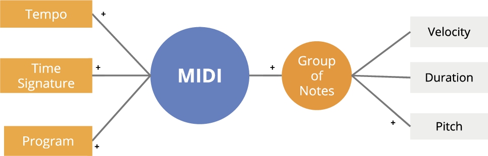
We propose a preliminary conversion of a MIDI file into a graph. As shown in Fig. 1, a MIDI node (the circle) represents the MIDI file and will be connected to nodes representing different parts of the MIDI content (i.e. tempo, programs, time signature, notes). A MIDI node can be linked to one or more nodes for each type.
Fig. 1.
Schema of the graph generated from MIDI. The + indicates edges representing connections of type many-to-many. The colours represent different groups of nodes: MIDI M (blue), Content C (orange) among which Notes N have a round shape, and Attributes A (grey).
In the context of graph embeddings computation, the practice is to take into account only connections between entities, that are nodes represented by identifiers. Literal values (text, numbers, etc.) are normally ignored [49] or some shrewdness is applied such as the use of contiguity windows [25]. In fact, literals can increase uncontrollably the number of nodes, in particular in presence of continuous values or entity-specific textual annotation. The effect is a very sparse graph,88 causing an exponential increment of the computation time and poor performance [40]. In our case, the crucial information represented as continuous data (e.g. the tempo) can not be excluded from the embeddings. We opted for partitioning the continuous values in ranges, in order to insert their information in the graph, while limiting at the same time the number of nodes. We provide some details for each type of node in the following.
Tempo, computed in
The continuous values are then discretised in partitions, each one representing a range of 10 bpm. Example: tempo-11 represents the range of values
Programs, representing the timbre of the channels, among the 128 different standard programs.99 Example: program-0 is the Acoustic Grand Piano.
Time signature is the measure of how many beats are contained in each measure. It is represented as the concatenation of numerator and denominator. Example:  is represented as ts-4/4.
Notes, representing the pitches in the MIDI. The information about duration and co-occurrence of notes (e.g. in a chord) are not directly represented in the MIDI file. The duration is extracted by comparing successive NoteOn and NoteOff events sharing the same pitch and located on the same channel. Co-occurring notes can be detected by comparing the same category of events among all channels, selecting the ones with overlapping Song Position Pointers (SPP). To include this information in the graph while limiting the number of nodes and edges, we extract all groups of notes starting (i.e. with a NoteOn message) at the same SPP. A tolerance of 10 ms is applied for considering two notes simultaneous, to overcome eventual small differences due to MIDI recording. Each group is connected to:
– the maximum duration of the notes in the group, discretised in classes of 100 ms. Example: the id duration-3 represents the range
– their average velocity. Example: velocity-1.
– all the pitches, identified by their standard MIDI numbers. Example: note-57 is A-3.
MIDI2vec does not encode any information concerning time, in particular about sequences of notes occurring in the same channel. This information is undoubtedly relevant and crucial in music representation. Nevertheless, we decide to not include the time dimension in this experiment for two main reasons. First, the inclusion of order and sequentiality in a graph representation is not very common and few works addressed this topic so far [45,54]. Second, this would require some choices, among them the number of consecutive notes to be grouped and the opportunity of representing pauses in the graph or not. For this reason, we decided to consider the encoding of subsequent notes for future work.
The connections between nodes are mostly of type many-to-many, so that two involved nodes are potentially part of other instances of the same connection. Taking as an example the connections between Tempo and MIDI types, this means that a specific Tempo node may be linked to different MIDI – pieces sharing the same tempo – and a specific MIDI may be linked to different tempos – representing a tempo change in the track. Some connections can be instead of type one-to-many: this is the case of the Group of Notes, linked to exactly one Duration which is, in turn, connected to several Group of Notes. Two MIDI nodes are never directly connected. Tempo, programs, and time signature might change within a file; we register all of them as equal nodes.
Formally, we realise a graph
Fig. 2.
MIDI graph example, showing possible connections between MIDI #1, #2, and #3.
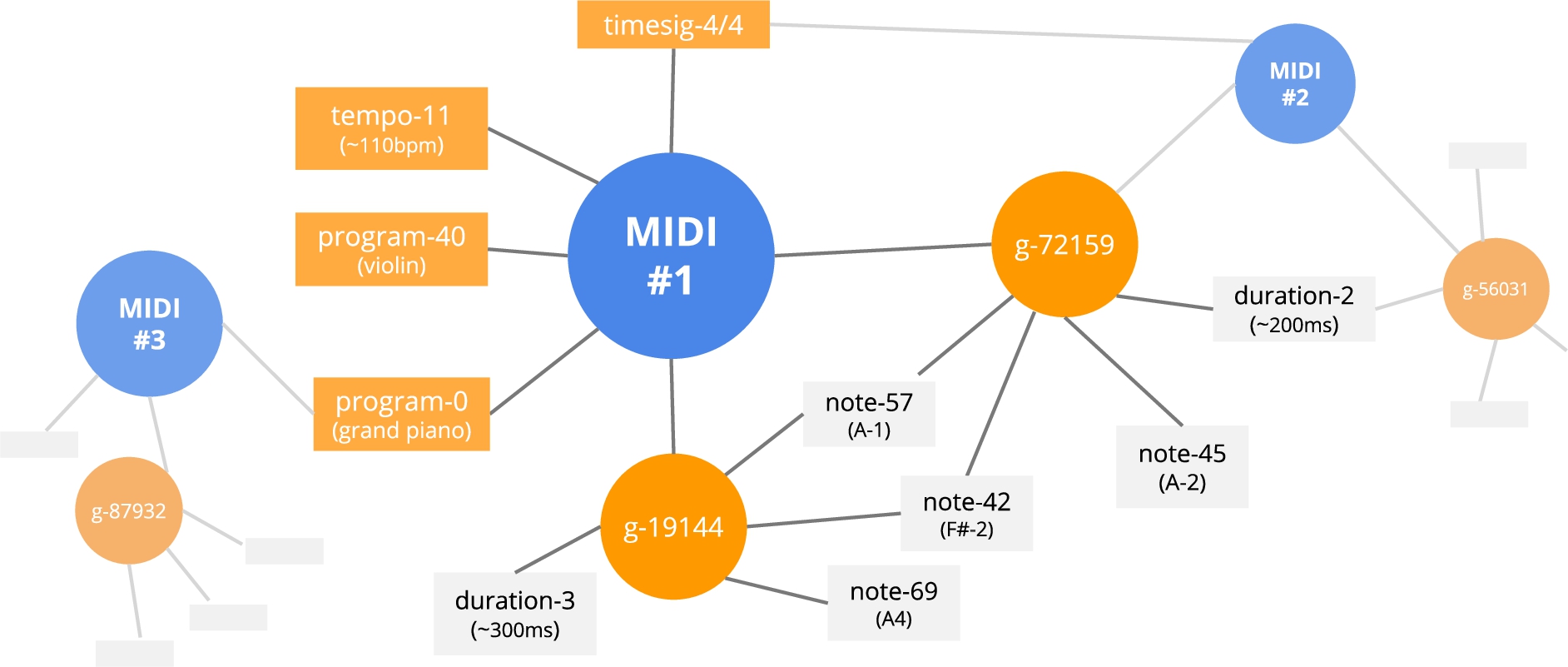
In Fig. 2, an excerpt of an example graph is provided, in particular showing the connections between MIDI files through complete note groups, single notes, duration, etc. In this kind of graph, two MIDI tracks sharing multiple chords (or other elements) will have more probability to appear in the same random walk. This representation aims to track at the same time the presence of specific chords and of quick and long notes, which can respectively characterise a more virtuous or lyrical composition.
The graph is saved in the edgelist format, which includes all couples of connected nodes. In the edgelist, each line of text represent an edge and contains the identifiers of the two involved nodes separated by blank spaces. In practice, the MIDI files are read and messages are sequentially converted and appended to the edgelist. This edgelist is the output of this first conversion and feeds the second part of the approach, described in the next section. Such obtained graph contains only information extracted from the MIDI content, not including any kind of external metadata.
4.2.Graph to vectors
Embeddings are computed on the output graph of the previous process with the node2vec algorithm. As more extensively written in Section 3, the algorithm simulates random walks on the graph and computes the transition probabilities between nodes, which are mapped into the vector space. In other words, two MIDI files sharing programs, tempos, note groups are more likely to be part of the same random walk and consequently are more likely to be close in the computed embedding space.
In practice, each node in the graph is selected as the starting node for a random walk, occupying its first slot. The second slot will be occupied by one of the nodes directly linked to the first node, according to the probability function. Iteratively, every slot of the random walk will be occupied by one of the neighbours of the previous one. The number of walks to be produced for each node and their length are given parameters. These walks are then processed by word2vec as they are sentences. The graph configuration, with few properties and densely connected nodes, make us prefer an approach based on random walks – representing similarities between nodes’ neighbourhoods – rather than those based on latent spaces of relations (e.g. TransE) [20].
Following this procedure, a 100-dimensions embedding vector is computed for each node (vertex) of the input graph. Each dimension of the vector cannot be attributed to a specific feature of the described item – for example, the tempo – but it rather represents latent features learned by the embedding algorithm. We apply a post-processing step in order to keep only the vectors
Such obtained vectors can be then used in input to algorithms, in tasks such as classification, clustering, and others. In the experiment which will be detailed in the following section, we will use such generated vectors in input to a neural network for classification. In particular, all vectors used in our experiment have been computed using the following configuration of node2vec: walk length = 10, number of walks = 40, window size = 5, number of iterations = 5,
5.Evaluation
We evaluate this strategy in relation to three different goals, involving three different MIDI datasets. These goals are detailed in the next sections and consist respectively in predicting the genre, some high-quality metadata, and some user-defined tags.
For each goal, we perform an experiment that relies on a common procedure. MIDI embeddings are generated on the dataset using MIDI2vec. A Feed-Forward Neural Network receives the MIDI embeddings as input (100 dimensions) in batches of size 32. The network is detailed in Fig. 3. The choice of a Feed-Forward NN is due to the fact that we do not capture the MIDI content as a temporal series – which would be necessary for working with CNN – but as a list of connections.
Fig. 3.
Scheme of the neural network.
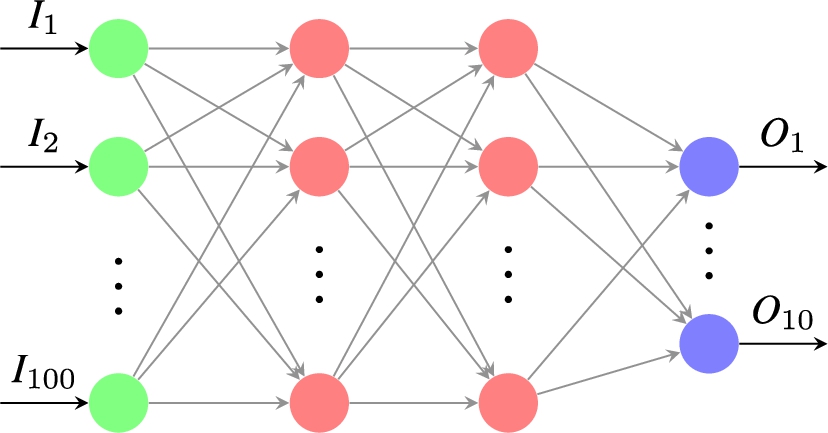
The set of labels used for training and testing changes according to each experiment. However, it is worth reminding the reader that those labels have not been used in the embedding task, and consequently, they are not directly included in the embedding information. The neural network consists of 3 dense layers. The hidden layers count 100 neurons each and use ReLU1010 as activation function. The output layer uses a sigmoid1111 as activation function and has a number of neurons equal to the dimension of the vocabulary of labels, which is represented with one-hot encoding. We performed 10-fold cross-validation1212 for training the neural network and we provide as final score the average of the accuracy1313 computed on every fold.
For the first two goals (Section 5.1 and 5.2), a further experiment requires a preliminary splitting of the dataset in 10 equal folds, in order to alternatively use 1 of them as test set and the remaining 9 as training set, implementing a complete 10-fold cross-validation (CCV). The embeddings are generated using exclusively the training set, while the vectors representing the MIDI files in the test set are computed a posteriori as the mean of the embeddings of their sibling elements in the graph (tempos, programs, note groups, time signatures). Even if this approach is not commonly applied and not equivalent to the result of embedding learning, we include this simplification to demonstrate how graph embedding information is generalisable to unseen data. In particular, we would like to prove that our system is not learning a hashing on the data but musically relevant features, demonstrating to not being a “horse” [56]. In the context of this experiment, the reported accuracy refers to the predictions on the test set generated by the neural network trained on the training set.
Currently, the library deals with the unpitched notes in MIDI Channel 10 (reserved to percussion by specification) as they have a pitch. When we ignore Channel 10 and use only programs representing pitched instruments,1414 we empirically observe that the average scores remain substantially unchanged (less than 1% of difference), while the standard deviation is around 2% higher. For this reason, we report here only the performances obtained considering note events from all channels.
These experiments are available as notebooks at https://git.io/midi-embs, which contains also the plots included in this paper in high resolution. Furthermore, all edgelists and learned embeddings for each dataset are also published for supporting research reproducibility at https://zenodo.org/record/5082300.
5.1.Genre prediction
In [30], McKay et al. perform a genre classification task on a contextually published SLAC Dataset,1515 which contains 250 MIDI files classified according to a two levels taxonomy. The first level includes 5 genre labels (Blues, Classical, Jazz, Rap, Rock), while the second one further specialises each genre by 2 sub-genres, for a total of 10 sub-genre labels. The dataset is perfectly balanced among the classes. Figure 4 shows a breakdown of the notes, instruments, tempo and time signature found in MIDIs of the SLAC dataset.
Fig. 4.
From left to right and top to bottom, notes, instruments, tempo and time signature of the MIDIs in the SLAC dataset (249 files). The average note is B3 (we have omitted all drum events in channel 10); the most frequent instruments (peaks) are acoustic grand piano, string ensemble 1, and distortion guitar. The average tempo is 203.16 bpm, estimated with [42]. The most common time signature is 4/4.
![From left to right and top to bottom, notes, instruments, tempo and time signature of the MIDIs in the SLAC dataset (249 files). The average note is B3 (we have omitted all drum events in channel 10); the most frequent instruments (peaks) are acoustic grand piano, string ensemble 1, and distortion guitar. The average tempo is 203.16 bpm, estimated with [42]. The most common time signature is 4/4.](https://content.iospress.com:443/media/sw/2022/13-3/sw-13-3-sw210446/sw-13-sw210446-g004.jpg)
We perform a 5-class genre classification experiment as well as a 10-class experiment on the same dataset. In [30], the authors use different inputs for predicting the genre: symbolic music (S) –which is the MIDI content–, lyrics (L), audio (A), cultural features (C) (tags extracted from the Web) and the multi-modal combination of all of these features (SLAC). In particular, the symbolic information is organised around 111 features (1021 dimensions). Their work has been extended and improved in a more recent paper [31] including, among others, features about chords and simultaneous notes, for a total of 172 features (1497 dimensions). We will compare our approach with these works, taking into account these 5 variants of features being used. The results are reported in Table 1.
Table 1
Accuracy of the genre classification. The reported values are the average (and standard deviation) of the cross-fold validation. In *N, *P, *T, *TS the embeddings have been computed on the sole notes, programs, tempos and time signature, while ALL includes all of them and *300 uses only the first 300 note-groups. Under CCV, the results of the complete cross-fold validation
| Approach | 5 classes | 10 classes | |
| McKay et al. 2010 [30] | S | 85% | 66% |
| L | 69% | 43% | |
| A | 84% | 68% | |
| C | 100% | 86% | |
| SLAC | 99% | 85% | |
| McKay et al. 2018 [31] | 93.2% | 77.6% | |
| MIDI2vec + NN | ALL | 86.4% (5.4%) | 67.2% (7.8%) |
| *N | 81.6% (7.6%) | 62.4% (9.9%) | |
| *P | 79.6% (6.8%) | 61.6% (8.6%) | |
| *T | 27.2% (9.5%) | 18.8% (9.2%) | |
| *TS | 25.6% (9.2%) | 15.2% (4.4%) | |
| *300 | 79.2% (7.0%) | 57.2% (12.5%) | |
| CCV | 76.8% (9.4%) | 55.2% (6.5%) | |
Our approach slightly outperforms [30] when only symbolic data are used in input (S), with an accuracy of 86% for 5-classes and 67% for 10-classes prediction. In addition, our method outperforms also other variants, namely lyrics (in both classes) and audio (in the 5-classes). The improvements made in [31] increase these scores by a few percentage points. We believe that the combination of melodic and chords features was crucial in this case and worth investigating in future work.
The same Table 1 shows also the accuracy scores obtained with different variations of the complete model (ALL); these variations compute the embeddings on the sole notes nodes (*N), program nodes (*P), tempo nodes (*T), and time signature nodes (*TS). None of these single features reaches the accuracy score of their combination. It is not surprising that *N reaches the higher accuracy among those models, having been computed on a more populated graph – the number of NoteOn/NoteOff events is higher than any other kind of event. Moreover, this study proves the absence of correlation between mono-dimensional features (e.g. tempo) and the classes. Finally, we trained the embeddings on all features, but taking into account only the first 300 note groups (*300). The experiment shows that reducing the number of vertexes in the graph causes lower accuracy scores.
Given the close results between the two best variations (ALL and *N), we studied their statistical significance, to understand if these two variations are likely to have the same accuracy mean. In order to do so, we extracted a t statistic computed on a 10 × 10-fold cross-fold validation, according to [6]. Applying this statistic to a Student’s t-test, we obtain their p-values, comparing them with the common significance level
In the complete cross-fold validation (CCV) experiment, the accuracy scores are around 10% lower. This decrease is mostly due to the difference in computing the vectors of the nodes in the train set (embedding algorithm) and the test set (average of other nodes). However, the results are consistent with respect to ALL, suggesting that the system is learning relevant features rather than coincidentally building a smart hashing on the content.
Fig. 5.
Confusion matrices of midi2vec predictions for the SLAC dataset.
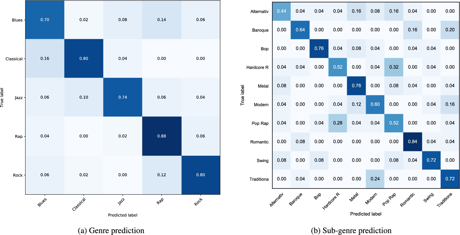
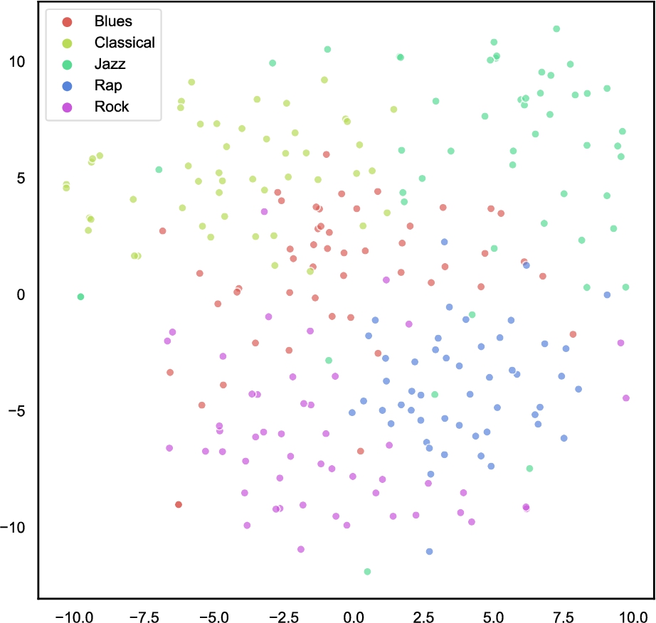
Figure 5 shows the confusion matrix between the real and the predicted values (configuration ALL). Even if there are no strong patterns, we can state that Blues is the genre that attracts more negative predictions. This is confirmed by what we see in Fig. 6, which contains a 2D visualisation of the vector space realised using the t-Distributed Stochastic Neighbor Embedding (t-SNE) algorithm1616 [58]. The final result is obtained by minimising the differences in this probability when computed on the low-dimensional space with respect to the high-dimensional one. In this figure, items of the same genre look closer in the space, with the Blues tracks occupying the central part of the graph, partially overlapping with the area of other genres. Figure 5b confirms that sub-genres belonging to the same parent genre are easier to be confused.
Fig. 6.
2D representation of the embedding space learned by midi2vec from the SLAC dataset.
5.2.Metadata prediction
This task consists in predicting a set of metadata from the MIDI, namely the composer, the genre, the instrument and the movement.
We started by downloading a corpus of 438 MIDI files from MuseData.1717 Those files refer to 139 classical music compositions, and each file can represent a specific movement. Figure 7 shows a breakdown of the notes, instruments, tempo and time signature found in MIDIs of the MuseData dataset.
Fig. 7.
From left to right and top to bottom, notes, instruments, tempo and time signature of the MIDIs in the MuseData dataset (439 files). The average note is E4 (we have omitted all drum events in channel 10); the most frequent instruments (peaks) are string ensemble 1, the acoustic grand piano, and the harpsichord. The average tempo is 188.96 bpm, estimated with [42]. The most common time signature is 4/4, with 3/4 also relatively frequent.
![From left to right and top to bottom, notes, instruments, tempo and time signature of the MIDIs in the MuseData dataset (439 files). The average note is E4 (we have omitted all drum events in channel 10); the most frequent instruments (peaks) are string ensemble 1, the acoustic grand piano, and the harpsichord. The average tempo is 188.96 bpm, estimated with [42]. The most common time signature is 4/4, with 3/4 also relatively frequent.](https://content.iospress.com:443/media/sw/2022/13-3/sw-13-3-sw210446/sw-13-sw210446-g007.jpg)
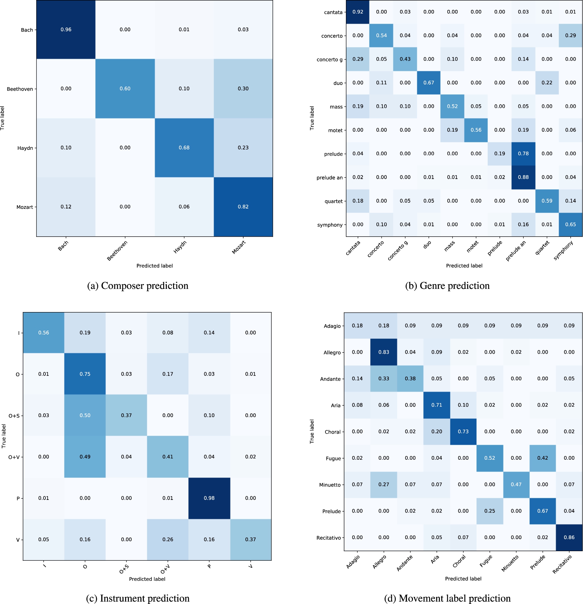
Fig. 8.
Confusion matrices of midi2vec predictions for the MuseData dataset. For the instrument predictions (c), the labels are Instrument, Orchestra, Orchestra + Soloist instrument, Orchestra + Voice, Piano, Voice.
MuseData provides also some metadata, like the composer name, the scholar catalogue number, a label for the movement. In order to obtain further information (i.e. the genre and the played instruments), we have interlinked each composition against the DOREMUS knowledge base [2], a dataset specialised in classical music metadata.
The interlinking process consists of three successive steps:
– interlinking of the composer through the exact match on the full name. This limits the candidates for the composition interlinking to the sole compositions of the interlinked composer;
– interlinking of the composition through the exact match on the catalogue number;
– if no catalogue number match is found, the titles are involved in the process. A title can often contain other kinds of information, such as key, instruments, opus number, etc. For example, the title “Symphony No. 3 in E-flat Major” contains the order number and the key. For this reason, titles are tokenised through empirical methods based on regular expressions to separate the different parts of the string, used as input of the Extended Jaccard Measure. [57]
Every composition can be linked to more than one MIDI file, in the case of works made of multiple movements. The movement labels have been cleaned by removing the order number, the key, the instruments and eventual comments in parentheses. For example, “1. Allegro in E Major” becomes simply “Allegro”.
The interlinking gives access to more specific metadata, mostly coming from controlled vocabularies [28], in particular composers (4 classes, i.e. Bach, Beethoven, Haydn, and Mozart), genres (10 classes), and instruments. For this last dimension, given the very large number of possibilities, we decided to reduce the number of classes to 6, including piano P, instrument (other than piano, including also small instrument ensembles) I, voice V, orchestra O, orchestra with voice O+V, and orchestra with instrumental soloist O+S. For instrument prediction, we excluded from the input, 21 MIDI with unknown instrumentation and 3 others that did not fall into any of the previous classes, having a final source dataset of 414 items.
Furthermore, we consider also the movement label as a feature to predict, considering only those which were occurring more than 10 times. Those labels include tempos (Allegro) and musical forms (Prelude), for a total of 9 distinct classes on 335 MIDI files. Some of these categories are loosely defined, but we consider them as-is since ambiguity is part of music information and therefore also part of the task. The dataset is not balanced among classes and has a strong presence of Bach works (76% of the total).
Table 2
For each kind of metadata feature, the table reports the number of items, the number of distinct classes, the average (and standard deviation) accuracy score for midi2vec, midi2vec with complete cross-validation, jSymbolic
| Feature | n. items | n. classes | midi2vec | midi2vec CCV | jSymbolic |
| Composer | 438 | 4 | 90.4% (5.8%) | 88.9% (15.0%) | 78.7% (4.9%) |
| Genre | 438 | 10 | 71.3% (6.4%) | 58.0% (16.6%) | 37.9% (9.3%) |
| Instrument | 414 | 6 | 65.1% (17.5%) | 48.6% (19.5%) | 46.1% (8.6%) |
| Movement | 335 | 9 | 68.3% (12.7%) | 54.9% (22.7%) | 32.4% (6.6%) |
The final accuracy (average of all the fold scores) is reported in Table 2. The best results are achieved for composer and genre prediction, and good results can be observed for all metadata. Looking at the confusion matrices:
– For the composers, the best results belong to Bach (the most present in the dataset). The two Austrian composers Mozart and Haydn are not surprisingly quite confused with one another, belonging both to the Classicism, differently from Beethoven (Classic-Romantic) and Bach (Baroque) [51]. The score for Beethoven reflect its under-representation (only 10 tracks) in the dataset (Fig. 8a);
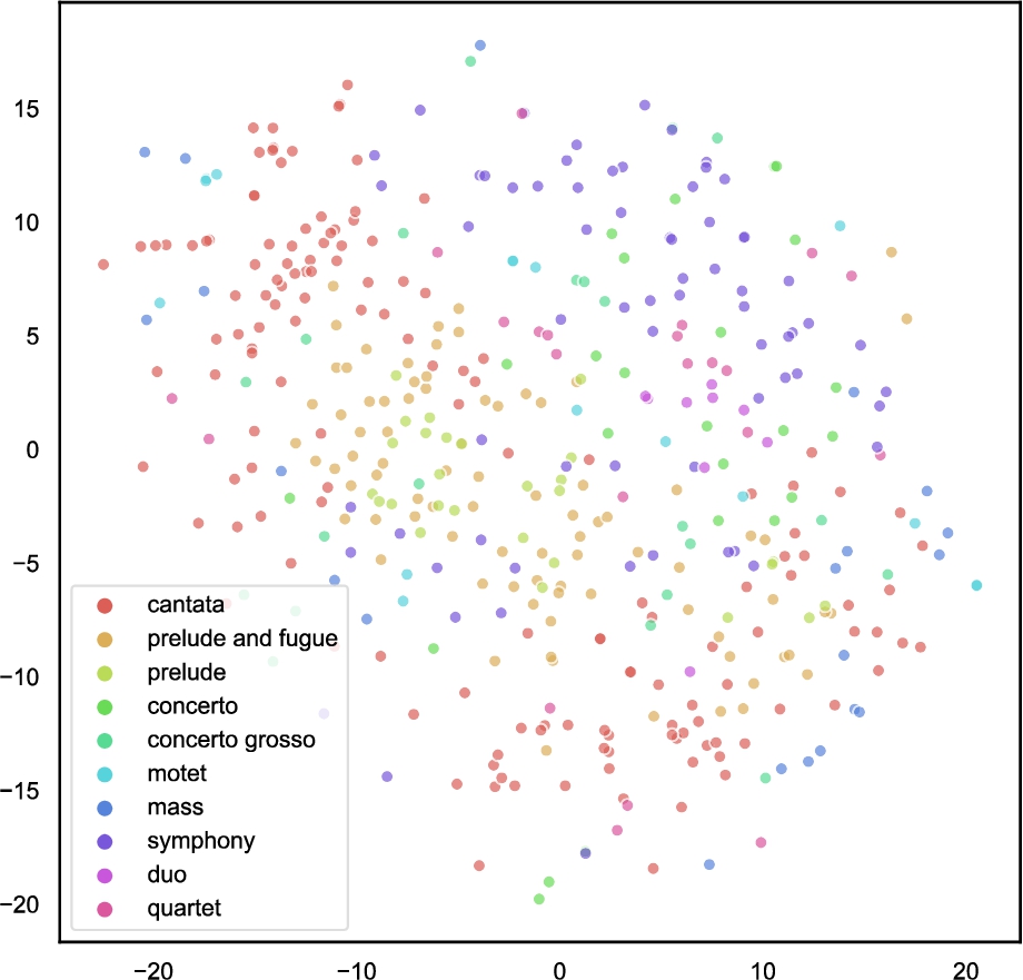
– The genres are much more specific than the ones investigated in Section 5.1. As a consequence, the greatest confusion occurs between couples of very similar genres, such as [concerto, symphony] and [prelude, prelude and fugue] (Fig. 8b). Those genre groups are overlapping also in the t-SNE visualisation in Fig. 9;
– While the instrument prediction has great results in identifying works for orchestra, piano solo or small ensemble of instruments, it reveals some unreliable classification for voice-only pieces, probably due to the under-representation of the class in the dataset. In the same way, the approach is not able to distinguish compositions for orchestra, orchestra and voice, and orchestra and soloist, all classified under the class O (Fig. 8c). This point has an important impact on the accuracy, which is lower than other metadata (instrument and movement) with a higher number of classes but more net differences between them;
– Even if the movement labels include heterogeneous meaning, the network correctly predicts 7 over 10 items. Some confusion patterns can be spotted. The Fugue tag is often predicted as Prelude, on the other hand proving a correct genre prediction. The classes representing tempos (e.g. Adagio or Tempo di Minuetto) are often confused with the most represented class among them (Allegro). Some confusion is visible also between the two tags related to singing, Aria and Choral (Fig. 8d).
Also in this case, we lose some accuracy (around 12-15%) when applying the complete cross-validation strategy. To have a comparison, we replicated the classification experiment described in [31], applying to Musedata an SVM classifier trained on the feature vectors computed by jSymbolic.1818 The results show how the features extracted from midi2vec are more capable to discern overlapping classes – e.g. genres of classical music, movement labels. We remind the reader that, in the studied dataset, there is no balance between classes, which may otherwise give even more significant results.
Fig. 9.
2D representation of the embedding space learned by midi2vec from the MuseData dataset.
5.3.Tag prediction
The Lakh MIDI Dataset (LMD)1919 is one of the biggest collections of MIDI which have been realised for research purposes [41]. An LMD-matched subset contains 31,0342020 MIDI aligned to entries of the Million Song Dataset, providing a set of metadata about the tracks, the albums and the artists. Figure 10 shows a breakdown of the notes, instruments, tempo and time signature found in MIDIs of the Lakh dataset.
Fig. 10.
From left to right and top to bottom, notes, instruments, tempo and time signature of the MIDIs in the Lakh dataset (31,036 files). The average note is B3 (we have omitted all drum events in channel 10); the most frequent instruments (peaks) are the acoustic grand piano, string ensemble 1, and acoustic guitar (steel). The average tempo is 213.15 bpm, estimated with [42]. The most common time signature is 4/4; 2/4 is also relatively frequent.
![From left to right and top to bottom, notes, instruments, tempo and time signature of the MIDIs in the Lakh dataset (31,036 files). The average note is B3 (we have omitted all drum events in channel 10); the most frequent instruments (peaks) are the acoustic grand piano, string ensemble 1, and acoustic guitar (steel). The average tempo is 213.15 bpm, estimated with [42]. The most common time signature is 4/4; 2/4 is also relatively frequent.](https://content.iospress.com:443/media/sw/2022/13-3/sw-13-3-sw210446/sw-13-sw210446-g010.jpg)
We extracted from LMD-matched two kinds of tags, coming respectively from MusicBrainz2121 and The Echo Nest.2222 The former group is a mix of terms that may refer to genres – i.e. classic pop – or to nationalities – British – while the latter group is more homogeneous in representing genres. Both kinds of tags refer more to the artist rather than to the exact track.
Differently from the experiment in Section 5.2, the size of the dataset allows to further filter the data to extract a balanced dataset. In particular, we select all distinct classes which are represented by at least 50 instances. For each of these classes, we randomly select 50 instances. Table 3 shows the accuracy for the predictions, measured through 10-fold cross-validation, together with the number of classes (distinct tags) against which we run the classification. In addition, in the table are reported the accuracy scores obtained by an SVM classifier built on top of jSymbolic. The comparison of these results reveals that latent features can largely boost the performance in tag classification, with evident benefit in real-world scenarios like automatic tag prediction.
Table 3
For each kind of tag feature, the table reports the number of items, the number of distinct classes, the average (and standard deviation) accuracy score for midi2vec and jSymbolic
| Feature | n. items | n. classes | midi2vec | jSymbolic |
| MusicBrainz | 2400 | 48 | 39.7% (2.8%) | 3.7% (1.4%) |
| EchoNest | 6800 | 136 | 32.5% (1.9%) | 1.4% (0.4%) |
The confusion matrices are shown in Fig. 11. Among the most wrongly predicted MusicBrainz classes, we find a strong presence of nationality tags (British, Italian, UK, etc.). The consistent number of classes make complicate to detect patterns in the confusion matrix, in which the best values are however concentrated in the diagonal of corrected predictions. To overcome this issue, we report in Table 4 the most frequent wrong predictions. For MusicBrainz tags, the list includes loosely defined genres (easy listening, ccm), one evident error (line 6.), together with couples of tags that can be considered similar or overlapping (1., 3., 7.). Looking at EchoNest tags, all pairings are meaningful, involving similar or related genres. This data gives us more confidence that the neural network is learning music-relevant features, which are well represented through graph embeddings.
Fig. 11.
Confusion matrices of midi2vec predictions for the Lakh dataset.
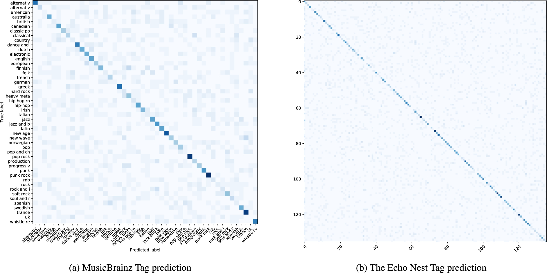
Table 4
Most frequent prediction errors for tag classification, with the percentage of cases over the total of the class
| Tag | Ground truth | Predicted | % | |
| MusicBrainz | 1. | ballad | folk rock | 12 |
| 2. | blues-rock | ccm | 12 | |
| 3. | classic rock | british invasion | 12 | |
| 4. | cool jazz | ccm | 10 | |
| 5. | easy listening | classic rock | 12 | |
| 6. | flamenco | british invasion | 12 | |
| 7. | folk rock | ballad | 10 | |
| EchoNest | 8. | orchestra | requiem | 10 |
| 9. | progressive trance | hard trance | 10 | |
| 10. | ragtime | jazz | 10 | |
| 11. | requiem | orchestra | 10 | |
| 12. | techno | tech house | 10 |
6.Conclusion and future work
In this paper, we hypothesise that symbolic music content in MIDI files, and its embedding representation in vector space, are a powerful tool for automated metadata classification tasks. Traditionally, applications of machine learning to this problem have encountered limitations in feature selection, and more recent embedding-based techniques have been only used for other tasks (e.g. music generation) or on different data (e.g. music metadata). In this paper, we propose MIDI2vec, a method to represent MIDI content as a graph and, subsequently, in a vector space through learning graph embeddings. We gather evidence that our hypothesis holds: MIDI2vec embeddings were successful in metadata classification, obtaining comparable performances to state-of-art methods based on feature extraction from symbolic music, with the added advantages of scalability, automating feature engineering, and reducing the required dimensions by one order of magnitude.
We plan on improving this work in various ways. Even if experiments revealed that the impact of unpitched notes in Channel 10 is minimal, we intend to assign a separated branch of the graph to percussion notes in the future, in order to distinguish them from the other ones while still taking them into account, with the goal of improving the overall performance.
Being transformed into a flat graph, the MIDI content loses in MIDI2vec all time-based information, with the only exception of simultaneity. Given the importance of melodic patterns in a music piece, future work would investigate how this work can deal with note sequences. We plan to investigate a few different strategies. First, sequences of notes may be encoded similarly to the simultaneous notes groups and included in MIDI2vec as a fifth node type. A second strategy may rely upon the inclusion in the graph embedding process of sequence embeddings like Sequence Graph Transform (SGT), which is capable of short- and long- term sequence features [45]. It is possible to think of MIDI file as a temporal graph, in which the information (currently played notes, tempo, playing instruments, etc.) evolves over time, and apply to such a graph temporal node embeddings strategies [54]. The instrument information (program) can be also combined with the pitch one, for describing the notes in all aspects.
Another study may combine MIDI2vec with other feature extraction techniques – e.g. the previously cited [31] – in an ensemble system, to exploit the best of the two methods. Finally, we would like to investigate if the learned features can be employed in predicting other kinds of data, for example the category of a videogame (adventure, shooting, fighting) from a dataset of soundtracks in MIDI [16].
A MIDI ontology and a corpus of over 300 thousand MIDI in RDF format have been presented in [33]. Despite being an interesting target for MIDI2vec, the extraction of crucial information (like the duration of a note) from the dataset is hard. In the current version, the ontology faithfully reproduces the event structure of the MIDI files, while significant edges – e.g. among simultaneous notes or consecutive events – are missing. Still, the MIDI2vec approach does not exploit edges between consecutive groups of notes, while they may potentially impact the performances. We plan to extend or map the MIDI ontology to solve this issue and enable MIDI2vec for working on such corpus, e.g. to perform link discovery and knowledge graph completion. In particular, crowdsourcing strategies on these resources may be applied to create large annotated datasets to use as ground truth. Moreover, it would be interesting to extend this approach to other symbolic music notation formats, namely MusicXML.
According to some intuition from other works in the genre classification field [9], the computation should not necessarily involve the full length of the track. Experiments with different time spans or sample sizes among the graph edges can help in detecting a trade-off between the performances and the embedding computation time. Recent approaches for including literal values in graph embeddings [11,27] could be included in MIDI2vec, to avoid any arbitrary choice that value-partitioning implies. Finally, we will use MIDI2vec in more applied contexts, such as the task of knowledge graph completion in knowledge bases with incomplete metadata entries [34].
Notes
1 We leave the interesting alternative of traversing these MIDI files sequentially, i.e. following the trail of temporal event occurrence instead of contextual co-occurrence, as future work.
6 Two nodes are connected if exists one or more paths of edges between them, of which the two edges represent respectively the first and the last node involved. A connection can consist of a single edge; in this case, we can speak about directly connected nodes.
7 A regularly updated list of software for embedding generation is available at https://github.com/MaxwellRebo/awesome-2vec.
8 A graph is considered dense or sparse if its number of edges is close or far, respectively, to the number of all potential edges connecting each pair of vertices [15].
9 The full list of MIDI programs is available at https://jazz-soft.net/demo/GeneralMidi.html.
10 A rectified linear unit (ReLU) is a classic activation function in Deep Learning networks, which return 0 when the input is negative or the input value itself when it is positive. ReLU is widely used because of its simplicity and its empirically demonstrated fast convergence.
11 The sigmoid function transforms the input x according to the formula:
12 In 10-fold cross-validation, the dataset is split into 10 groups, choosing in sequence each of them as test set (10%) and the remaining 9 as training set (90%).
13 The definition of accuracy is “the closeness of agreement between a test result and the accepted reference value”, i.e. the true value (ISO 5725-1).
14 Musical instruments can be classified as pitched, producing recognisable notes in the musical scale (e.g. the piano), or unpitched, producing sounds of indefinite pitch (e.g. the cymbals).
15 SLAC dataset: http://jmir.sourceforge.net/Codaich.html.
16 Similarly to Principal Components Analysis (PCA), t-SNE maps a high-dimensional space into a low-dimensional one. The algorithm computes the probability that a point A would choose point B as its neighbour, according to a Gaussian probability distribution centred at A.
17 The MuseData dataset is available on the old musedata website: http://old.musedata.org.
18 We also used the jSymbolic vectors in combination with a Neural Network, but obtaining worse performance scores.
19 Lakh MIDI Dataset: https://colinraffel.com/projects/lmd/.
20 The LMD website declares that LMD-matched includes 45,129 MIDIs. However, only 31,034 of them have metadata within an HDF5 file.
21 MusicBrainz: https://musicbrainz.org/.
22 The Echo Nest: http://the.echonest.com/.
Acknowledgements
This work is partly supported by the CLARIAH project funded by the Dutch Research Council NWO. This work is part of a project that has received funding from the European Union’s Horizon 2020 Research and Innovation Programme under grant agreement No. 101004746 (Polifonia: a digital harmoniser for musical heritage knowledge, H2020-SC6-TRANSFORMATIONS).
References
[1] | R. Abboud and J. Tekli, MUSE prototype for music sentiment expression, in: IEEE International Conference on Cognitive Computing (ICCC), San Francisco, CA, USA, (2018) , pp. 106–109. doi:10.1109/ICCC.2018.00023. |
[2] | M. Achichi, P. Lisena, K. Todorov, R. Troncy and J. Delahousse, DOREMUS: A graph of linked musical works, in: 17th International Semantic Web Conference (ISWC), Monterey, CA, USA, (2018) . doi:10.1007/978-3-030-00668-6_1. |
[3] | A. Allik, G. Fazekas and M.B. Sandler, An ontology for audio features, in: 17th International Society for Music Information Retrieval Conference (ISMIR), New York, NY, USA, (2016) . |
[4] | M.M. Association, The complete MIDI 1.0 detailed specification, Los Angeles, CA, USA, pp. 1996–2014, Technical Report, MIDI Manufacturers Association, https://www.midi.org/specifications/item/the-midi-1-0-specification. |
[5] | D. Bogdanov, N. Wack, E. Gómez Gutiérrez, S. Gulati, P. Herrera Boyer, O. Mayor, G. Roma Trepat, J. Salamon, J.R. Zapata González and X. Serra, Essentia: An audio analysis library for music information retrieval, in: 14th International Society for Music Information Retrieval Conference (ISMIR), Curitiba, Brazil, (2013) . |
[6] | R.R. Bouckaert and E. Frank, Evaluating the replicability of significance tests for comparing learning algorithms, in: Advances in Knowledge Discovery and Data Mining (PAKDD), H. Dai, R. Srikant and C. Zhang, eds, Springer, Berlin, Heidelberg, (2004) , pp. 3–12. ISBN 978-3-540-24775-3. doi:10.1007/978-3-540-24775-3_3. |
[7] | M. Buffa, E. Cabrio, M. Fell, F. Gandon, A. Giboin, R. Hennequin, F. Michel, J. Pauwels, G. Pellerin, M. Tikat and M. Winckler, The WASABI dataset: Cultural, lyrics and audio analysis metadata about 2 million popular commercially released songs, in: 18th Extended Semantic Web Conference (ESWC) – Resources Track, Springer International Publishing, Cham, (2021) , pp. 515–531. doi:10.1007/978-3-030-77385-4_31. |
[8] | M.A. Casey, R. Veltkamp, M. Goto, M. Leman, C. Rhodes and M. Slaney, Content-based multimedia information retrieval: Current directions and future challenges, Proceedings of the IEEE 96: (4) ((2008) ), 668–696. doi:10.1109/JPROC.2008.916370. |
[9] | Z. Cataltepe, Y. Yaslan and A. Sonmez, Music genre classification using MIDI and audio features, EURASIP Journal on Advances in Signal Processing 2007: (1) ((2007) ), 036409. doi:10.1155/2007/36409. |
[10] | O. Celma and X. Serra, FOAFing the music: Bridging the semantic gap in music recommendation, Web Semantics: Science, Services and Agents on the World Wide Web 6: (4) ((2008) ), 250–256. doi:10.1016/j.websem.2008.09.004. |
[11] | M. Cochez, M. Garofalo, J. Lenßen and M.A. Pellegrino, A first experiment on including text literals in KGloVe, in: 4th Workshop on Semantic Deep Learning (SemDeep), Monterey, CA, USA, (2018) . |
[12] | F. Colombo, J. Brea and W. Gerstner, Learning to generate music with BachProp, in: 16th Sound and Music Computing Conference (SMC), Malaga, Spain, (2019) , pp. 380–386. |
[13] | D.C. Corrêa and F.A. Rodrigues, A survey on symbolic data-based music genre classification, Expert Systems with Applications 60: ((2016) ), 190–210, http://www.sciencedirect.com/science/article/pii/S095741741630166X. doi:10.1016/j.eswa.2016.04.008. |
[14] | M.S. Cuthbert, C. Ariza and L. Friedland, Feature extraction and machine learning on symbolic music using the music21 toolkit, in: 12th International Society for Music Information Retrieval Conference (ISMIR), Porto, Portugal, (2011) . |
[15] | R. Diestel, Graph Theory, Graduate Texts in Mathematics, Vol. 173: , Springer, (2005) . doi:10.1007/978-3-662-53622-3. |
[16] | C. Donahue, H.H. Mao and J. McAuley, The NES music database: A multi-instrumental dataset with expressive performance attributes, in: 19th International Society for Music Information Retrieval Conference (ISMIR), Paris, France, (2018) . |
[17] | Z. Fu, G. Lu, K.M. Ting and D. Zhang, A survey of audio-based music classification and annotation, IEEE Transactions on Multimedia 13: (2) ((2011) ), 303–319. doi:10.1109/TMM.2010.2098858. |
[18] | J. Gomez, J. Abeßer and E. Cano, Jazz solo instrument classification with convolutional neural networks, source separation, and transfer learning, in: 19th International Society for Music Information Retrieval Conference (ISMIR), Paris, France, (2018) . |
[19] | P. Goyal and E. Ferrara, Graph embedding techniques, applications, and performance: A survey, Knowledge-Based Systems 151: ((2018) ), 78–94. doi:10.1016/j.knosys.2018.03.022. |
[20] | M. Grohe, Word2vec, node2vec, graph2vec, x2vec: Towards a theory of vector embeddings of structured data, in: 39th ACM SIGMOD-SIGACT-SIGAI Symposium on Principles of Database Systems, PODS’20, Association for Computing Machinery, New York, NY, USA, (2020) , pp. 1–16. ISBN 9781450371087. doi:10.1145/3375395.3387641. |
[21] | A. Grover and J. Leskovec, Node2vec: Scalable feature learning for networks, in: 22nd ACM SIGKDD International Conference on Knowledge Discovery and Data Mining (KDD), San Francisco, CA, USA, (2016) . doi:10.1145/2939672.2939754. |
[22] | I. Guyon and A. Elisseeff, An introduction to variable and feature selection, Journal of Machine Learning Research 3: ((2003) ), 1157–1182. |
[23] | Z.S. Harris, Distributional structure, 1954, pp. 146–162, WORD 10(2–3). doi:10.1080/00437956.1954.11659520. |
[24] | A. Huang and R. Wu, Deep learning for music, Computing Research Repository (CoRR) (2016), abs/1606.04930. |
[25] | M. Kejriwal and P. Szekely, Neural embeddings for populated geonames locations, in: 16th International Semantic Web Conference (ISWC), Springer International Publishing, Vienna, Austria, (2017) , pp. 139–146. ISBN 978-3-319-68204-4. doi:10.1007/978-3-319-68204-4_14. |
[26] | F. Korzeniowski and G. Widmer, Genre-agnostic key classification with convolutional neural networks, in: 19th International Society for Music Information Retrieval Conference (ISMIR), Paris, France, (2018) . |
[27] | A. Kristiadi, M. Asif Khan, D. Lukovnikov, J. Lehmann and A. Fischer, Incorporating literals into knowledge graph embeddings, in: The Semantic Web – ISWC 2019, Springer International Publishing, Cham, (2019) , pp. 347–363. ISBN 978-3-030-30793-6. doi:10.1007/978-3-030-30793-6_20. |
[28] | P. Lisena, K. Todorov, C. Cecconi, F. Leresche, I. Canno, F. Puyrenier, M. Voisin and R. Troncy, Controlled vocabularies for music metadata, in: 19th International Society for Music Information Retrieval Conference (ISMIR), Paris, France, (2018) . |
[29] | P. Lisena and R. Troncy, Combining music specific embeddings for computing artist similarity, Suzhou, China, 2017. |
[30] | C. McKay, J. Burgoyne, J. Hockman, J.B.L. Smith, G. Vigliensoni and I. Fujinaga, Evaluating the genre classification performance of lyrical features relative to audio, symbolic and cultural features, in: 11th International Society for Music Information Retrieval Conference (ISMIR), Utrecht, The Netherlands, (2010) . |
[31] | C. McKay, J.E. Cumming and I. Fujinaga, jSymbolic 2.2: Extracting features from symbolic music for use in musicological and MIR research, in: 19th International Conference on Music Information Retrieval, ISMIR, Paris, France, (2018) . |
[32] | C. McKay and I. Fujinaga, Automatic genre classification using large high-level musical feature sets, in: 5th International Conference on Music Information Retrieval (ISMIR), Barcelona, Spain, (2004) . |
[33] | A. Meroño-Peñuela, M. Daquino and E. Daga, A large-scale semantic library of MIDI linked data, in: 5th International Conference on Digital Libraries for Musicology (DLfM), Paris, France, (2018) . |
[34] | A. Meroño-Peñuela, R. Hoekstra, A. Gangemi, P. Bloem, R. de Valk, B. Stringer, B. Janssen, V. de Boer, A. Allik, S. Schlobach et al., The MIDI Linked Data Cloud, in: 16th International Semantic Web Conference (ISWC), Springer, Vienna, Austria, (2017) , pp. 156–164. doi:10.1007/978-3-319-68204-4_16. |
[35] | T. Mikolov, K. Chen, G. Corrado and D. Jeffrey, Efficient estimation of word representations in vector space, in: 1st International Conference on Learning Representations (ICLR), Workshop Track, Scottsdale, AZ, USA, (2013) , http://arxiv.org/abs/1301.3781. |
[36] | A. Narayanan, M. Chandramohan, R. Venkatesan, L. Chen, Y. Liu and S. Jaiswal, graph2vec: Learning distributed representations of graphs, in: 13th International Workshop on Mining and Learning with Graphs (MLG), (2017) . |
[37] | E. Palumbo, D.M.G. Rizzo, R. Troncy and E. Baralis, entity2rec: Property-specific knowledge graph embeddings for item tecommendation, Expert Systems with Applications 151: ((2020) ), 113235. doi:10.1016/j.eswa.2020.113235. |
[38] | J. Pennington, R. Socher and C. Manning, GloVe: Global vectors for word representation, in: Empirical Methods in Natural Language Processing (EMNLP), Association for Computational Linguistics, Doha, Qatar, (2014) , pp. 1532–1543. doi:10.3115/v1/D14-1162. |
[39] | B. Perozzi, R. Al-Rfou and S. Skiena, DeepWalk: Online learning of social representations, in: 20th ACM SIGKDD International Conference on Knowledge Discovery and Data Mining (KDD), ACM, New York, NY, USA, (2014) , pp. 701–710. ISBN 978-1-4503-2956-9. doi:10.1145/2623330.2623732. |
[40] | J. Pujara, E. Augustine and L. Getoor, Sparsity and noise: Where knowledge graph embeddings fall short, in: Conference on Empirical Methods in Natural Language Processing (EMNLP), Association for Computational Linguistics, (2017) , pp. 1751–1756, http://aclweb.org/anthology/D17-1184. doi:10.18653/v1/D17-1184. |
[41] | C. Raffel, Learning-based methods for comparing sequences, with applications to audio-to-MIDI alignment and matching, Phd thesis, Columbia University, 2016. |
[42] | C. Raffel and D.P. Ellis, Intuitive analysis, creation and manipulation of MIDI data with pretty_midi, in: 15th International Conference on Music Information Retrieval (ISMIR), Late Breaking Demo, Taipei, Taiwan, (2014) , pp. 84–93. |
[43] | C. Raffel and D.P.W. Ellis, Extracting ground truth information from MIDI files: A MIDIfesto, in: 17th International Society for Music Information Retrieval Conference (ISMIR), New York, NY, USA, (2016) . |
[44] | Y. Raimond, S.A. Abdallah, M.B. Sandler and F. Giasson, The music ontology, in: 15th International Conference on Music Information Retrieval (ISMIR), Vienna, Austria, (2007) , pp. 417–422. |
[45] | C. Ranjan, S. Ebrahimi and K. Paynabar, Sequence Graph Transform (SGT): A feature extraction function for sequence data mining, 2016, arXiv preprint arXiv:1608.03533. |
[46] | S. Rashid, D. De Roure and D. McGuinness, A music theory ontology, in: 1st International Workshop on Semantic Applications for Audio and Music (SAAM), ACM, Monterey, CA, USA, (2018) , pp. 6–14. ISBN 978-1-4503-6495-9. doi:10.1145/3243907.3243913. |
[47] | A. Ratner, S.H. Bach, H. Ehrenberg, J. Fries, S. Wu and C. Ré, Snorkel: Rapid training data creation with weak supervision, in: Proceedings of the VLDB Endowment. International Conference on Very Large Data Bases, Vol. 11: , NIH Public Access, (2017) , p. 269. doi:10.14778/3157794.3157797. |
[48] | A. Ratner, C. De Sa, S. Wu, D. Selsam and C. Ré, Data programming: Creating large training sets, quickly, in: 30th International Conference on Neural Information Processing Systems (NIPS), NIPS’16, Curran Associates Inc., Red Hook, NY, USA, (2016) , pp. 3574–3582. ISBN 9781510838819. |
[49] | P. Ristoski, J. Rosati, T. Di Noia, R. De Leone and H. Paulheim, RDF2Vec: RDF graph embeddings and their applications, Semantic Web Journal 10: (4) ((2019) ), 721–752. doi:10.3233/SW-180317. |
[50] | A. Roberts, J. Engel, C. Raffel, C. Hawthorne and D. Eck, A hierarchical latent vector model for learning long-term structure in music, in: 35th International Conference on Machine Learning (ICML), Proceedings of Machine Learning Research, Vol. 80: , PMLR, Stockholmsmässan, Sweden, (2018) , pp. 4364–4373. |
[51] | C. Rosen, The Classical Style: Haydn, Mozart, Beethoven, WW Norton & Company, (1997) . ISBN 0393317129. |
[52] | P.E. Schreur and N. Lorimer, Linked data in libraries’ technical services workflows, in: Metadata and Semantic Research, Springer International Publishing, Cham, (2017) , pp. 224–229. ISBN 978-3-319-70863-8. doi:10.1007/978-3-319-70863-8_21. |
[53] | S. Si-Said Cherfi, C. Guillotel, F. Hamdi, P. Rigaux and N. Travers, Ontology-based annotation of music scores, in: Knowledge Capture Conference (K-CAP), ACM, Austin, TX, USA, (2017) , pp. 10:1–10:4. ISBN 978-1-4503-5553-7. doi:10.1145/3148011.3148038. |
[54] | U. Singer, I. Guy and K. Radinsky, Node embedding over temporal graphs, in: 28th International Joint Conference on Artificial Intelligence (IJCAI), IJCAI Organization, (2019) , pp. 4605–4612. doi:10.24963/ijcai.2019/640. |
[55] | S. Song, M. Kim, S. Rho and E. Hwang, Music ontology for mood and situation reasoning to support music retrieval and recommendation, in: 3rd International Conference on Digital Society (ICDS), IEEE, Cancun Mexico, (2009) , pp. 304–309. doi:10.1109/ICDS.2009.50. |
[56] | B.L. Sturm, A simple method to determine if a music information retrieval system is a “horse”, IEEE Transactions on Multimedia 16: (6) ((2014) ), 1636–1644. doi:10.1109/TMM.2014.2330697. |
[57] | A.N. Tigrine, Z. Bellahsene and K. Todorov, Light-weight cross-lingual ontology matching with LYAM++, in: On the Move to Meaningful Internet Systems Conferences (OTM), Springer International Publishing, Rhodes, Greece, (2015) , pp. 527–544. ISBN 978-3-319-26148-5. doi:10.1007/978-3-319-26148-5_36. |
[58] | L. van der Maaten and G. Hinton, Visualizing data using t-SNE, Journal of machine learning research 9: (v) ((2008) ), 2579–2605. |
[59] | R. van der Weerdt, Generating music from text: Mapping embeddings to a VAE’s latent space, Master’s thesis, University of Amsterdam, 2018. |
[60] | D. Weigl, W. Goebl, T. Crawford, A. Gkiokas, N. Gutierrez, A. Porter, P. Santos, C. Karreman, I. Vroomen, C.C.S. Liem, A. Sarasúa and M. van Tilburg, Interweaving and enriching digital music collections for scholarship, performance, and enjoyment, in: 6th International Conference on Digital Libraries for Musicology (DLfM), Association for Computing Machinery, New York, NY, USA, (2019) , pp. 84–88. ISBN 9781450372398. doi:10.1145/3358664.3358666. |
[61] | L. Weng, Are deep neural networks dramatically overfitted?, lilianweng. github. io/lil-log (2019), http://lilianweng.github.io/lil-log/2019/03/14/are-deep-neural-networks-dramatically-overfitted.html. |
[62] | X. Wilcke, P. Bloem and V. De Boer, The knowledge graph as the default data model for learning on heterogeneous knowledge, Data Science 1: (1–2) ((2017) ), 39–57. doi:10.3233/DS-170007. |
[63] | T. Wilmering, G. Fazekas and M.B. Sandler, AUFX-O: Novel methods for the representation of audio processing workflows, in: 15th International Semantic Web Conference (ISWC), Springer International Publishing, Kobe, Japan, (2016) , pp. 229–237. ISBN 978-3-319-46547-0. doi:10.1007/978-3-319-46547-0_24. |
[64] | Y. Yan, E. Lustig, J. VanderStel and Z. Duan, Part-invariant model for music generation and harmonization, in: 19th International Society for Music Information Retrieval Conference (ISMIR), Paris, France, (2018) . |


