
Multidimensional enrichment of spatial RDF data for SOLAP
Abstract
Large volumes of spatial data and multidimensional data are being published on the Semantic Web, which has led to new opportunities for advanced analysis, such as Spatial Online Analytical Processing (SOLAP). The RDF Data Cube (QB) and QB4OLAP vocabularies have been widely used for annotating and publishing statistical and multidimensional RDF data. Although such statistical data sets might have spatial information, such as coordinates, the lack of spatial semantics and spatial multidimensional concepts in QB4OLAP and QB prevents users from employing SOLAP queries over spatial data using SPARQL. The QB4SOLAP vocabulary, on the other hand, fully supports annotating spatial and multidimensional data on the Semantic Web and enables users to query endpoints with SOLAP operators in SPARQL. To bridge the gap between QB/QB4OLAP and QB4SOLAP, we propose an RDF2SOLAP enrichment model that automatically annotates spatial multidimensional concepts with QB4SOLAP and in doing so enables SOLAP on existing QB and QB4OLAP data on the Semantic Web. Furthermore, we present and evaluate a wide range of enrichment algorithms and apply them on a non-trivial real-world use case involving governmental open data with complex geometry types.
1.Introduction
Data warehouses (DWs) and Online Analytical Processing (OLAP) tools and queries are widely used for interactive data analysis. DWs have multidimensional (MD) models and store large volumes of data. MD models locate data in an n-dimensional space and are usually referred to as data cubes. The cells of a cube represent the topic of the analysis and associate observation facts with (numerical) measures that can be aggregated. Spatial data cubes can also contain spatial measures, which can be aggregated with spatial functions. For example, a data cube for farms might have a numerical measure ‘number of animals’ as well as the ‘farm’s coordinates’ as spatial measure. Facts are linked to dimensions, which provide contextual information, e.g., farm production, farm location, and farm livestock. Dimensions are organized into hierarchies with levels, e.g., parish of the farm or herd type of livestock, which allow users to analyze and aggregate measures at different levels of detail. Levels have a set of attributes describing the characteristics of the level members.
In traditional DWs, the location dimension is generally used as a conventional (non-spatial) dimension with alphanumeric data and thus provided with only a nominal reference to places and areas, e.g., parish name. This does not allow for applying spatial operations or truly deriving topological relations between hierarchy levels based on geometric information such as coordinates, which are essential for enabling spatial OLAP (SOLAP) analysis.
By including the geometric information of locations in MD models, we can significantly improve the analysis process (e.g., proximity analysis of locations) with additional perspectives by revealing dynamic spatial hierarchy levels and new spatial level members in SOLAP operations (details and examples in [14,15]). In addition, by using geometric attributes of level members, topological relations between the levels, and levels and facts can be specified implicitly. Such topological relations are essential to correctly aggregate measures between levels with many-to-many (N:M) cardinality relations, for instance.
The Semantic Web (SW) has evolved, from prominently focusing on data publishing to also supporting complex queries, such as interactive analytical queries. Simultaneously, the data available on the SW has evolved from being simple, mostly alphanumerical data, to include complex data types, such as geospatial data. There are many examples of governmental and statistical Linked Open Data (LOD) sets with geographical attributes. However, such datasets are typically not modeled with multidimensional concepts. Thus, they cannot be queried with interactive analytical queries (OLAP). Although in recent years several platforms and tools for Business Intelligence (BI) and data warehouses have emerged [50], there is still a lack of common standards to model and publish (geo)semantic cubes on the SW [15].
More and more statistical datasets using the RDF Data Cube Vocabulary (QB) [48], the current W3C standard, are published on the SW. These datasets have observations and measures, which are well-suited for analytical queries. However, QB lacks the underlying structural metadata for multidimensional models and OLAP operations (Section 6). Well-defined structural metadata is required to translate OLAP queries into SPARQL 1.1 [14,46]. QB4ST [3] is a recent attempt to define extensions for spatio-temporal components to QB. However, it inherits the limitations of multidimensional modeling from QB.
To address the MD modeling challenges of the QB vocabulary, QB4OLAP [7] has been proposed, which reuses QB definitions by adding the required MD schema semantics. A significant number of data sets have already been published using the QB vocabulary. QB4OLAP descriptions of a QB data cube can be generated semi-automatically by adding the necessary MD semantics (e.g., the hierarchical structure of the dimensions) and the corresponding instances to populate the dimension levels. However, existing QB4OLAP annotation techniques [44] only cover non-spatial MD data cube concepts and its operations. Even though such statistical data sets have spatial information, not annotating the spatial MD concepts (e.g., spatial hierarchy levels such as administrative regions) hinders querying the data with interesting spatial OLAP operations. To emerge this need the QB4SOLAP vocabulary was proposed [13], which allows modeling the data cubes fully with both multidimensional and spatial concepts on the SW.
Fig. 1.
Future vision of SOLAP on the SW.
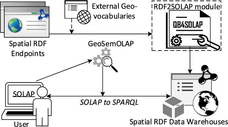
Problem motivation and definition Spatial OLAP (SOLAP) queries are currently not well supported by existing spatial RDF stores and endpoints. Instead, the user would have to a) download the (maybe very large) RDF data, b) map it to a relational schema (e.g., a snowflake schema), c) import it into a traditional spatial data warehouse, d) make all queries and analyses within the traditional spatial DW, and finally e) import and map any results and knowledge back into the original RDF store. This obviously is a slow, labor-intensive, and error-prone process, which furthermore completely locks out the vast majority of users without advanced programming skills.
Luckily, there already exist tools and vocabularies for (spatial) data warehouses on the SW: the QB4SOLAP vocabulary [13], for instance, allows publishing data with spatial multidimensional concepts on the SW and provides high-level SOLAP operators that can be translated into SPARQL [15]. Based on these, GeoSemOLAP [14] enables users to issue SOLAP queries on geo-semantic RDF data without detailed knowledge of SPARQL or RDF.
GeoSemOLAP, however, is restricted to RDF data sets that are already annotated with QB4SOLAP.
Thus, there is a great unmet need for an automated approach to enrich and annotate geo-semantic RDF data from existing endpoints with QB4SOLAP metadata. This is exactly what our proposed RDF2SOLAP enrichment module does (Fig. 1).
Since on-the-fly annotations would require the corresponding heavy spatial operations to be executed repeatedly for each new query, making response times too slow for interactive OLAP querying, we annotate the entire data set in a once-and-for-all fashion.
Contributions In summary, the main contributions of this paper are:
* An illustration of the need for QB4SOLAP, i.e., the need to enable fully-fledged data warehouse concepts for geo-semantic RDF data. We further introduce running examples from real-world governmental open data on environment and farming with complex geometry types.
* A detailed explanation and comparison of RDF data examples, which are depicted as graphs, and annotated both with QB4OLAP and QB4SOLAP vocabularies, then identifying the required spatial MD metadata and concepts (e.g., spatial hierarchies and topological relations) for SOLAP analysis based on the given comparison.
* Hierarchical enrichment algorithms for (1) detecting topological relations at hierarchy steps with direct links between the level members; and (2) discovering topological relations at hierarchy steps (which do not have direct links between the level members).
* Factual enrichment algorithms for fact-level relations between fact and level members.
* An automated way of re-defining a fact schema after factual enrichment, and association of spatial aggregate functions with spatial measures.
* General implementation of our approach for both hierarchical enrichment and factual enrichment processes.
* Evaluation of our approach in terms of accuracy and coverage in comparison to two standard environments (RDBMS and GIS tool).
Paper organization The remainder of this paper is organized as follows. Section 2 defines the preliminary concepts used throughout the paper with a running use case example. Section 3 presents the system architecture for the MD enrichment process. Section 4 defines the RDF2SOLAP enrichment algorithms with necessary helper functions and formalization of (spatial) RDF data. The Appendix presents the implementation details along with interesting examples and discusses the challenges and implemented solutions. Section 5 presents the qualitative and performance evaluation with comparison baselines. Finally, Section 6 discusses related work and Section 7 concludes the paper with an outlook to future work.
2.Preliminaries
In this section, we explain the preliminary concepts of spatial data warehouses and SOLAP (Section 2.1) and how to deploy them on the Semantic Web (Section 2.2) using the QB4SOLAP vocabulary.
2.1.Spatial data warehouses and SOLAP
Data cubes and spatially extended cube concepts Data warehouses (DW) are based on a multidimensional model that models data in an n-dimensional space – often referred to as a data cube. A cube schema defines the structure of a cube with MD concepts. The cells of the cube represent (observation) facts with a set of attributes called measures. Facts are linked to dimensions, which are the axes of an MD space and provide perspectives to analyze the data. Dimensions are organized into hierarchies, which allow users to aggregate measures at different granularities along the levels of a hierarchy. Hierarchies are composed of levels, which have a set of attributes describing the characteristics of the level members. Each level member is defined by its attributes and attribute values.
Cube members are MD concepts that are defined at the instance level and composed of level members, attributes of level members, partial order on level members, and fact members. A hierarchy step between levels (a child level and a parent level) defines a set of roll-up relations, where each relation relates a child level member to a parent level member. These roll-up relations define a partial order between level members with a cardinality relation. The cardinality (1:1, 1:N, N:1, N:M) describes the number of members in one level that can be related to a member in the other level for both child and parent levels.
Spatial data warehouses (SDW) extend a DW by storing geometries such as point, line, and polygon in the values of spatial measures and values of level attributes for spatial dimensions. The spatially extended MD schema of an SDW has spatial dimensions, spatial hierarchies, spatial levels [29], spatial hierarchy steps, and topological relations (in addition to cardinality relations) between spatial levels for each spatial hierarchy step [13]. Topological relations are Boolean spatial predicates that specify how two spatial objects are related to each other, e.g., within, intersects, touches, crosses and etc. [6]. Similar to conventional DWs, facts of an SDW can be associated with numeric measures, which are using aggregation functions such as SUM, AVG, etc. A fully extended spatial MD schema of an SDW should also define spatial measures, which have geometries and spatial aggregate functions. Spatial aggregate functions aggregate two or more spatial objects and return a new spatial object. Union, Intersection, ConvexHull, and Minimum-BoundingRectangle (MBR) are example of spatial aggregate functions. For a detailed explanation of SDW concepts we refer the reader to [42].
Fig. 2.
GeoFarmHerdState – parish, farm, and drainage area instances.
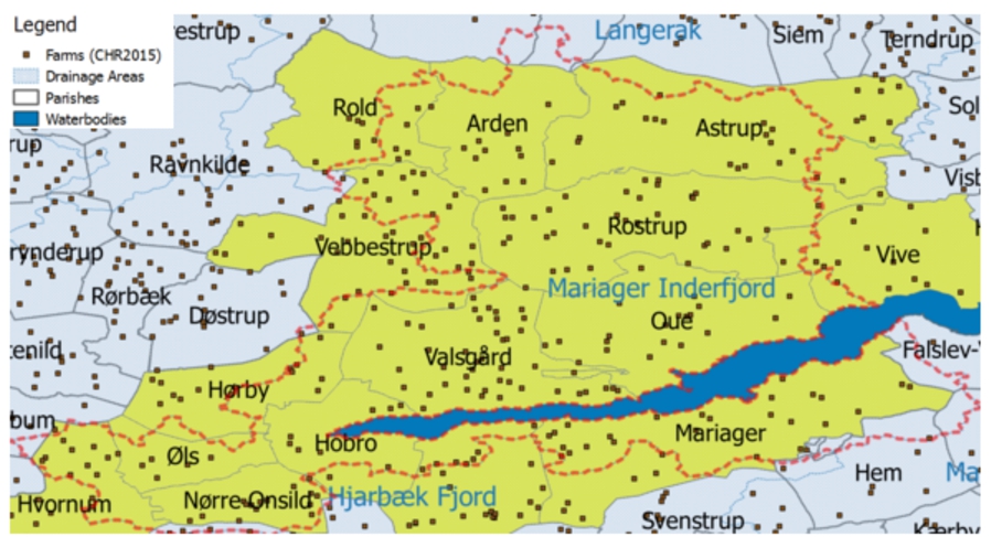
Fig. 3.
GeoFarmHerdState – conceptual MD schema of livestock holdings data (spatial concepts).
OLAP and spatial OLAP operations DWs are commonly used to store large volumes of data for decision support with On-Line Analytical Processing (OLAP) operations. Spatial OLAP (SOLAP) integrates the features of OLAP tools and geographical information systems (GIS) [38]. SOLAP enables advanced analytical processing by taking the spatial information in the cube into account.
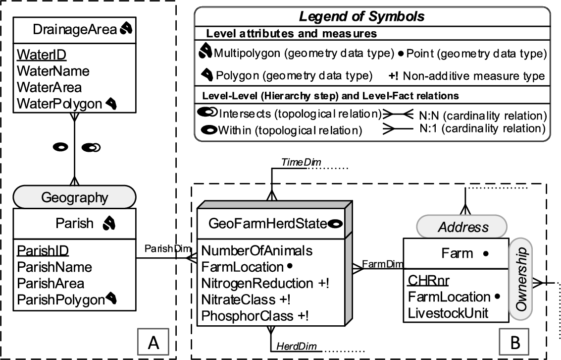
For example, a spatial data cube of livestock holdings in farms (referred to as GeoFarmHerdState in the rest of this paper) defines the farm location as a spatial measure, which is linked to the observation facts. In order to derive perspectives and relations on the state of the farms’ livestock holdings (herds), spatial levels are defined: parishes and drainage areas. A sample set of the corresponding spatial data cube members are given in Fig. 2. The spatial MD concepts of the data cube are defined in the conceptual schema in Fig. 3, which depicts a simplified version of the GeoFarmHerdState spatial data cube without its non-spatial dimensions (see [12] for further details the GeoFarmHerdState cube). The cube has two spatial dimensions: FarmDim and ParishDim. The latter has a spatial hierarchy (Geography) with two spatial levels: Parish and DrainageArea. FarmDim on the other hand does not have a spatial hierarchy, despite its spatial (base) level: Farm.
The GeoFarmHerdState cube has spatial fact members for farms within a time frame and different kinds of measures, i.e., numeric measures: NumberofAnimals in the farm and NitrogenReduction potential of the farm land/soil, spatial measures: FarmLocation (Fig. 3).11
To evaluate SOLAP operations, spatial levels such as Parish and DrainageArea are used to aggregate measures at different levels of detail. Due to the polygon geometry of the spatial level members, there are two different roll-up relations for the hierarchy step between the Parish and DrainageArea levels, where a parish can be completely contained within a drainage area or a parish and a drainage area can intersect.
For example, parish “Oue” is within drainage area “Mariager Inderfjord”. Thus, all the farms that are within “Oue” are also within “Mariager Inderfjord”. Whereas, parish “Astrup” intersects with drainage areas “Mariager Inderfjord” and “Langerak”. Therefore, some farms that are within “Astrup” are within “Mariager Inderfjord”, while the rest of the farms are within “Langerak”. Figure 2 displays a sample set of Parish and DrainageArea level members.
The possible roll-up relations for the example above are depicted in Fig. 4 with black and red arrows representing the topological relations within and intersects. Blue arrows show the topological relation contains, which are drill-down (inverse operation of roll-up) relations from DrainageArea level to Farm level.
Topological relations between levels and facts can be implicitly specified through the geometry attributes of their instances (level members and fact members). The relations between spatial levels enable processing spatial roll-up and drill-down through range queries with spatial predicates [8]. In terms of cardinality, there is an N:M relationship between level members since a parish may intersect with more than one drainage area and vice versa. This induces the problem of computing measures incorrectly when a roll-up operation goes through an N:M relationship, which actually is the case between the Parish level and the DrainageArea level. For example, we would like to aggregate the measure NumberOfAnimals, from Parish level to the DrainageArea level with a roll-up query. In such a roll-up query, we might falsely aggregate the number of animals in farms that are contained within the parish, but not contained within the drainage area, since the parish intersects with another drainage area. In order to refine such an analysis, SOLAP operations are required, where a (spatial) drill-down should be applied to the lowest granularity – from Parish level members to GeoFarmHerdState fact members, and then a spatial roll-up (with within predicate) can be applied from fact members (Farm instances) to DrainageArea level members. This would prevent falsely aggregating the number of animals from the farms that are (spatially) disjoint to the corresponding drainage area.
Fig. 4.
Hierarchy example for SOLAP.
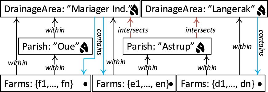
Fig. 5.
Hierarchy steps in QB4OLAP before multidimensional enrichment.
2.2.QB4SOLAP: Spatial RDF data cube vocabulary for SOLAP operations
There is an increasing amount of Linked Open Data (LOD) on the Semantic Web containing spatial information and numerical (statistical) data. This led to new opportunities for OLAP over spatial data using semantic web technologies and standards. Datasets on the SW use a standardized format: RDF (Resource Description Framework).22
In order to enable SOLAP operations on the Semantic Web, a comprehensive vocabulary is needed, i.e., annotation of the spatial hierarchy steps with topological relations. QB4SOLAP [15] is a vocabulary that allows the definition of cube schemas and cube instances in RDF. The QB4SOLAP vocabulary is an extension of QB4OLAP [7] capturing the semantics of spatial MD concepts (i.e., spatial hierarchy steps) that are essential for SOLAP operations. The QB4SOLAP vocabulary V1.3 is available on our project website33 as well as via a persistent URL.44
A comprehensive foundation of spatial data warehouses on the Semantic Web can be found in [15], which includes detailed definitions with semantics of spatial MD concepts both at the schema level and instance level using QB4SOLAP.
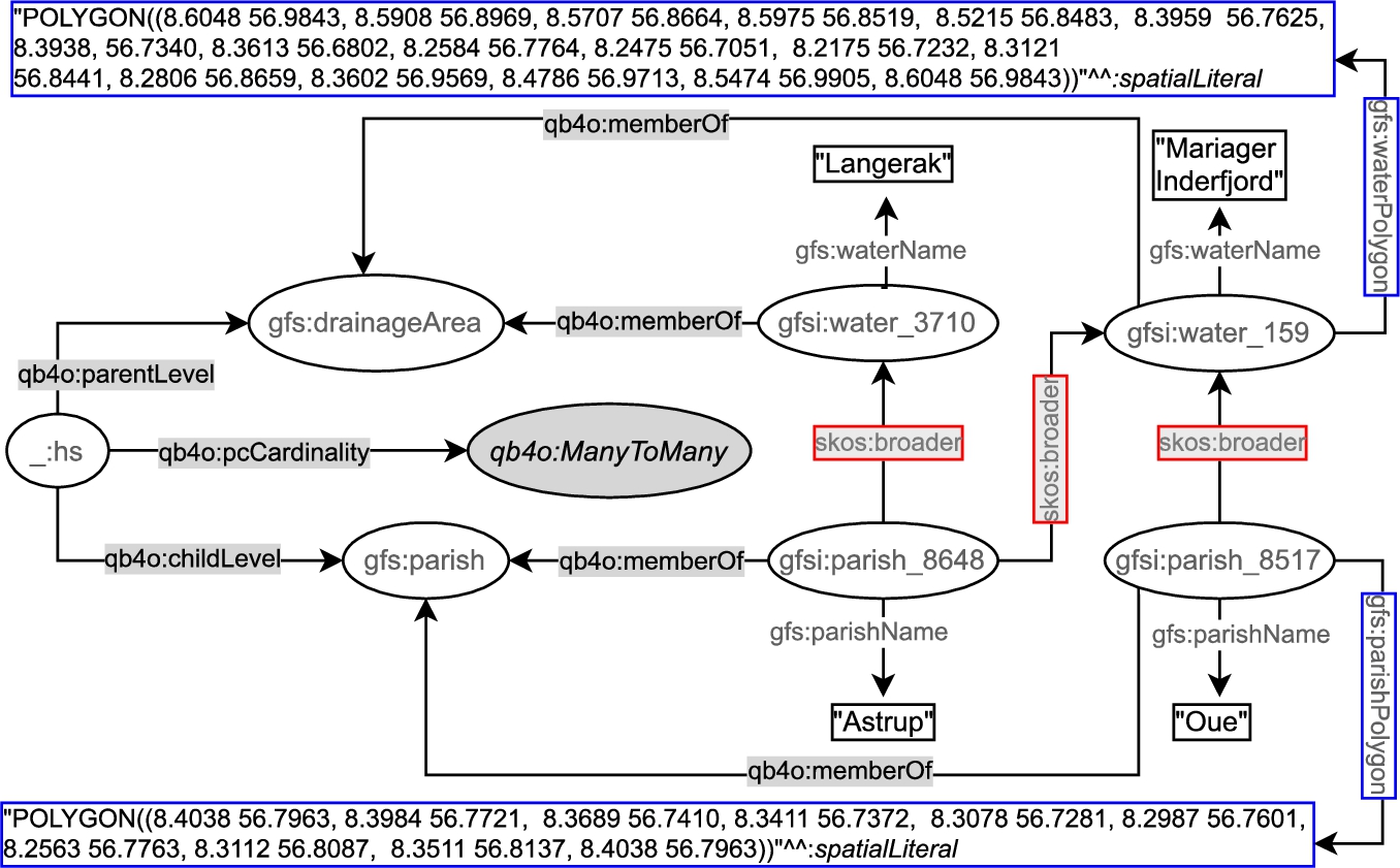
In the following, we depict an example of a hierarchy step from gfs:Parish child level to gfs:drainageArea parent level (Fig. 5). In the figure, we prefix the schema elements (attributes, levels, etc.) of the (GeoFarmHerdState) cube with gfs: and instance data from the cube with gfsi:. The left-center part of Fig. 5 shows the hierarchy structure _:hs, between gfs:parish and gfs:drainageArea levels at the schema level with the QB4OLAP vocabulary. QB4OLAP objects, classes, and properties are prefixed with qb4o:. The levels (gfs:parish and gfs:drainageArea) are linked to the instances of level members (e.g., gfsi:parish_8648, gfsi:water_3710 and etc.) by qb4o:memberOf property. The polygon geometry attributes are highlighted in blue boxes, on the top and the bottom of the figure. The coordinates recorded in the geometry attributes can be used to derive the topological relation between the level members by applying spatial boolean predicates (e.g., instersects?, within?) on the polygon geometries of the parish and drainage area level members.
However, QB4OLAP does not support annotating the topological relations that might exist between the level members at a hierarchy step. QB4OLAP uses only skos:broader property from SKOS (Simple Knowledge Organization System) [30] semantic relations for capturing the roll-up relations at hierarchy steps. The roll-up relations with skos:broader property are highlighted in red boxes in Fig. 5. The skos:broader property does not describe the nature of the roll-up relation with topological relations for spatial hierarchies. Therefore, QB4OLAP cannot capture the topological relations in a hierarchy step from Parish level to DrainageArea level or between these levels’ members.
Fig. 6.
Spatial hierarchy steps in QB4SOLAP after multidimensional enrichment.
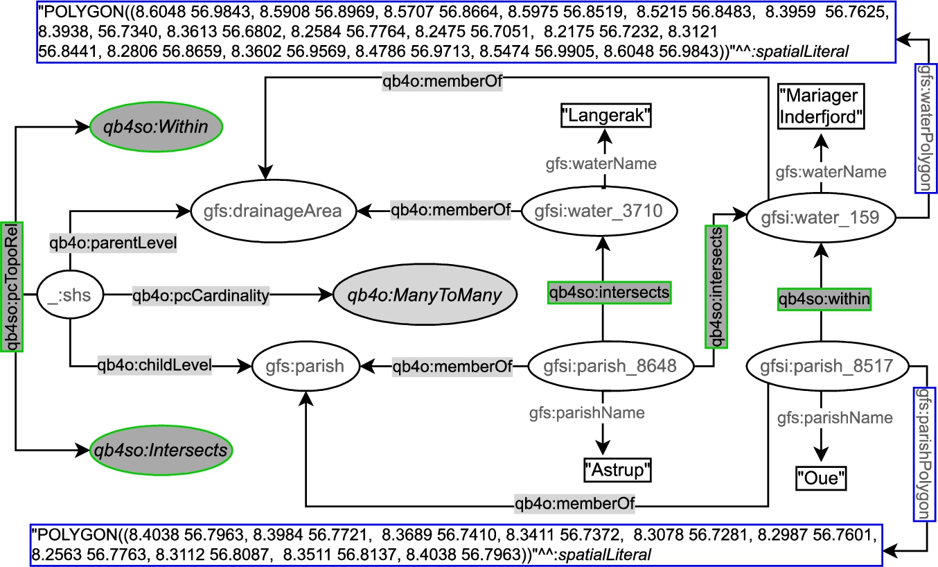
On the other hand, QB4SOLAP can define topological relations both at the schema level and the instance level. In Fig. 6, we prefix QB4SOLAP objects, classes, and properties with qb4so: and highlight them in green lines. The left-center part of the figure shows the spatial hierarchy structure :_shs, which has a QB4SOLAP property qb4so:pcTopoRel with two QB4SOLAP class instances qb4so:Within and qb4so:Intersects. This means that when we compare the geometry attributes of parish level members and drainage area level members, we discover two different topological relations (within and intersects) for all the (spatial) hierarchy steps between the parish and drainage area levels. And these relations are annotated at the schema level on the left-center part of Fig. 6.
Similarly, gfs:parish and gfs:drainageArea levels are linked to the instances of level members (e.g., gfsi:parish_8648) by qb4o:memberOf property. The explicit topological relations between each level member along a spatial hierarchy step are depicted in the figure with qb4so:intersects or qb4so:within predicates, which are highlighted in green boxes (e.g., gfsi:parish_8648 intersects with gfsi:water_159 and gfsi:water_3170 etc.).
In conclusion, QB4SOLAP enables SOLAP operations by defining the semantics of spatial MD concepts both at the schema level and instance level. These semantics are essential for SOLAP operations, and they are defined as extensions to the QB4OLAP vocabulary.
3.System architecture
The importance of SOLAP to get accurate results in operations over spatial data warehouses is explained in Section 2.1. However, the RDF data cubes (with spatial attributes) on the Semantic Web are not always annotated with vocabularies that allow users to formulate SOLAP queries. In this section we present an overview of the MD enrichment flow from RDF QB to QB4OLAP data cubes and QB4OLAP to QB4SOLAP data cubes. Thus, users can query the RDF data cubes with SOLAP queries.
Fig. 7.
Multidimensional enrichment process.
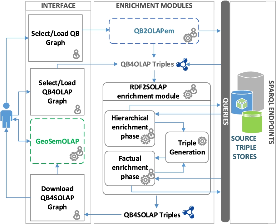
A multidimensional enrichment process flow is illustrated in Fig. 7 with three main architectural layers: Interface, Enrichment Modules, and SPARQL Endpoints. The architectural layers in the figure are denoted in horizontal rectangles. The first layer facilitates user interaction with the enrichment modules (i.e., QB2OLAPem) and third party tools (i.e., GeoSemOLAP). In each layer, processes are given in right angle boxes, modules and tools are given in rounded corner boxes. Third party tools and modules are annotated in dashed lines. Arrows in the figure represents the interaction between processes and the modules.
Our main contribution in this paper is the RDF2SOLAP enrichment module, which is the core of the second layer. The RDF2SOLAP enrichment module operates on QB4OLAP triples that either already exist in the original data or have been generated by the QB2OLAPem enrichment module [44]. QB2OLAPem allows users to enrich an RDF QB dataset with QB4OLAP concepts and returns a graph of QB4OLAP triples.
The internal process flow of the RDF2SOLAP enrichment module consists of three phases: hierarchical enrichment, factual enrichment, and triple generation. The hierarchical and factual enrichment phases iteratively perform the enrichment algorithms explained in Section 4. Hierarchical enrichment phase and factual enrichment phase can run independently from each other in parallel. Factual enrichment phase additionally can suggest an enriched fact schema definition, which depends on the spatial relations found at the instance level enrichment for factual and hiearchical enrichment phases. Both of these enrichment phases allow interaction with external SPARQL endpoints to enhance the enrichment process via potential spatial and multidimensional concepts that could be retrieved externally. The third phase is the triple generation, which creates QB4SOLAP triples that can be used in third party tools such as GeoSemOLAP. GeoSemOLAP allows users without knowledge of RDF and SPARQL to query with SOLAP operations by interactively formulating the queries using a GUI with interactive maps [14].
The third layer (SPARQL endpoints) allows interaction between user and SPARQL endpoint for retrieving QB or QB4OLAP graphs as well as interaction between system and SPARQL endpoints, where the RDF2SOLAP enrichment module queries external triple stores for hierarchical enrichment and factual enrichment.
RDF2SOLAP is implemented in Javascript on the Node.js platform using the N3.js library for parsing the RDF triples in Javascript and the Turfjs library for spatial analysis.55
4.RDF2SOLAP enrichment algorithms
This section presents the core algorithms of our RDF2SOLAP enrichment module. Our MD enrichment approach builds upon QB4OLAP triples that either already exist in the original data or have been generated by the QB2OLAPem enrichment module [44] as depicted in Fig. 7. QB4OLAP defines only the non-spatial multidimensional semantics of RDF data, whereas QB4SOLAP enriches the MD semantics of RDF data with spatial concepts (formalizations and further details can be found in [15]). Nevertheless, in the following we briefly introduce basic notations.
The basic construct of RDF is a triple
We define function
The MD enrichment process in RDF2SOLAP runs in two phases (hierarchical enrichment phase and factual enrichment phase), which are explained in the following.
4.1.Hierarchical enrichment phase
The hierarchical enrichment phase is built around spatial levels and their level members forming the spatial hierarchy of a dimension. Thus, by identifying the spatial relations between spatial levels and their level members, we can find the spatial hierarchy steps and the possible topological relations for these hierarchy steps.
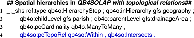
Each spatial hierarchy corresponds to a path of roll-up relationships between the child level and parent level: each of these roll-up relationships corresponds to a spatial hierarchy step (Section 2.1). An example of a (spatial) hierarchy with QB4SOLAP is given in Listing 1. Line 4 extends the QB4OLAP schema definitions by enriching the hierarchy step with the possibility to annotate the spatial hierarchy steps with topological relations (see Section 2 for details and Section 2.2 for examples).
Listing 1.
Spatial hierarchy structure in QB4SOLAP
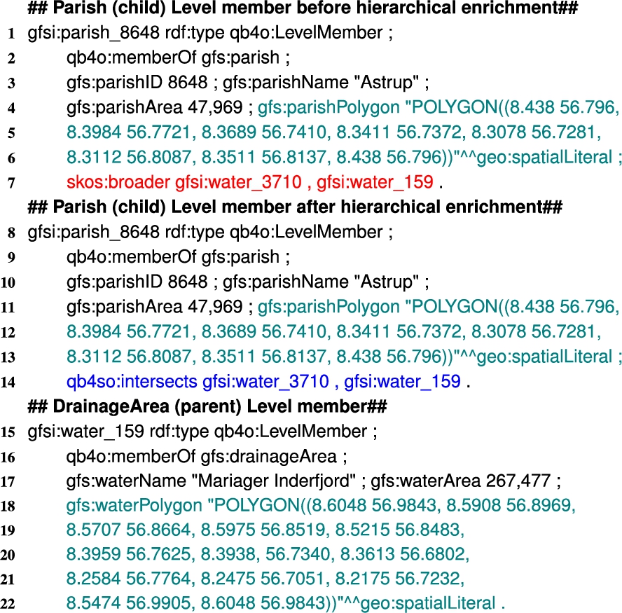
Listing 2 shows the GeoFarmHerdState spatial level members from Parish and Drainage Area levels. Lines 1–7 (Listing 2) represent the QB4OLAP annotation of a child level member from Parish level before multidimensional enrichment (with skos:broader), which is depicted in Fig. 5. Lines 8–14 represent the QB4SOLAP annotation of the same Parish level member after the multidimensional enrichment with topological relations (depicted in Fig. 6). Lines 15–22 represent the annotation of a parent level member from the Drainage area level, which remains the same before and after multidimensional enrichment since the hierarchy steps are defined with bottom-up relationships from child level to parent level and the roll-up relations and thus also the topological relations are annotated at the child level members of the hierarchy step.
Listing 2.
GeoFarmHerdState level members, attributes, and spatial roll-up relations
We exploit QB4OLAP semantics, such as non-spatial hierarchy steps and levels as a starting point to find the spatial hierarchy steps. We distinguish two cases:
Case 1: Finding explicit spatial hierarchy steps for QB4OLAP levels, with skos:broader roll-up relations between their child-parent level members by detecting spatial hierarchy steps in Section 4.1.2. For this case we assume that level members have direct skos:broader relations as depicted in Fig. 5 and Listing 2, Line 7 with skos:broader property.
Case 2: Finding implicit spatial hierarchy steps from QB4OLAP levels without direct roll-up relations through the skos:broader property. In this case, we assume that the level members are only defined by the qb4o:memberOf property as shown in Listing 2, (Line 2) but do not have the skos:broader roll-up relation as given in Line 7. In this case, it is still possible to discover spatial hierarchy steps by finding spatial (topological) relations between level members through their attributes as explained in Section 4.1.3.
4.1.1.Spatial helper functions
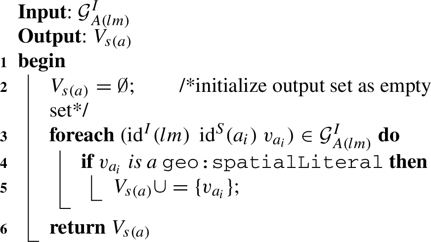
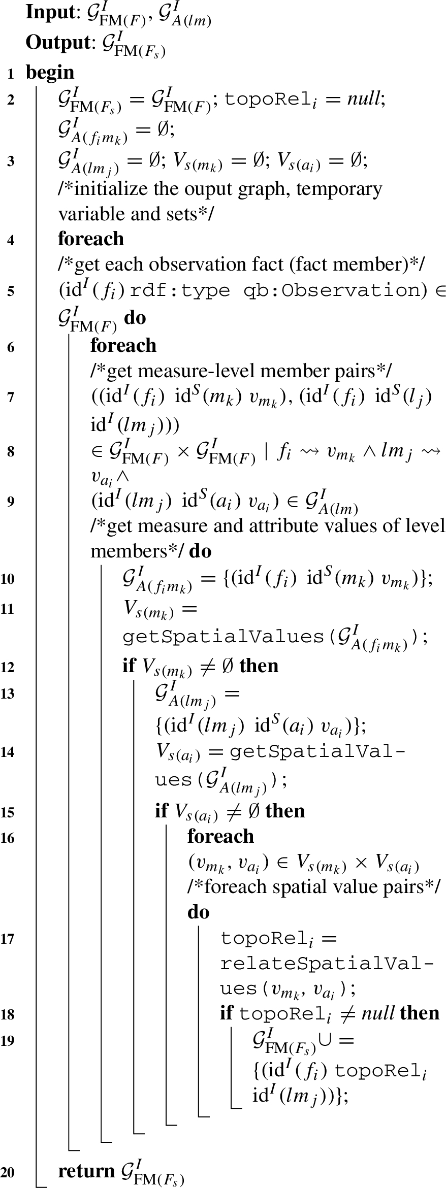
To address the cases explained above, we need two spatial helper functions; for retrieving spatial attribute values (Algorithm 1, getSpatialValues), and for relating spatial attributes (Algorithm 2, relateSpatialValues).
Algorithm 1 (getSpatialValues) The first helper function gets an input graph of attributes of level members
Algorithm 1
Algorithm 2
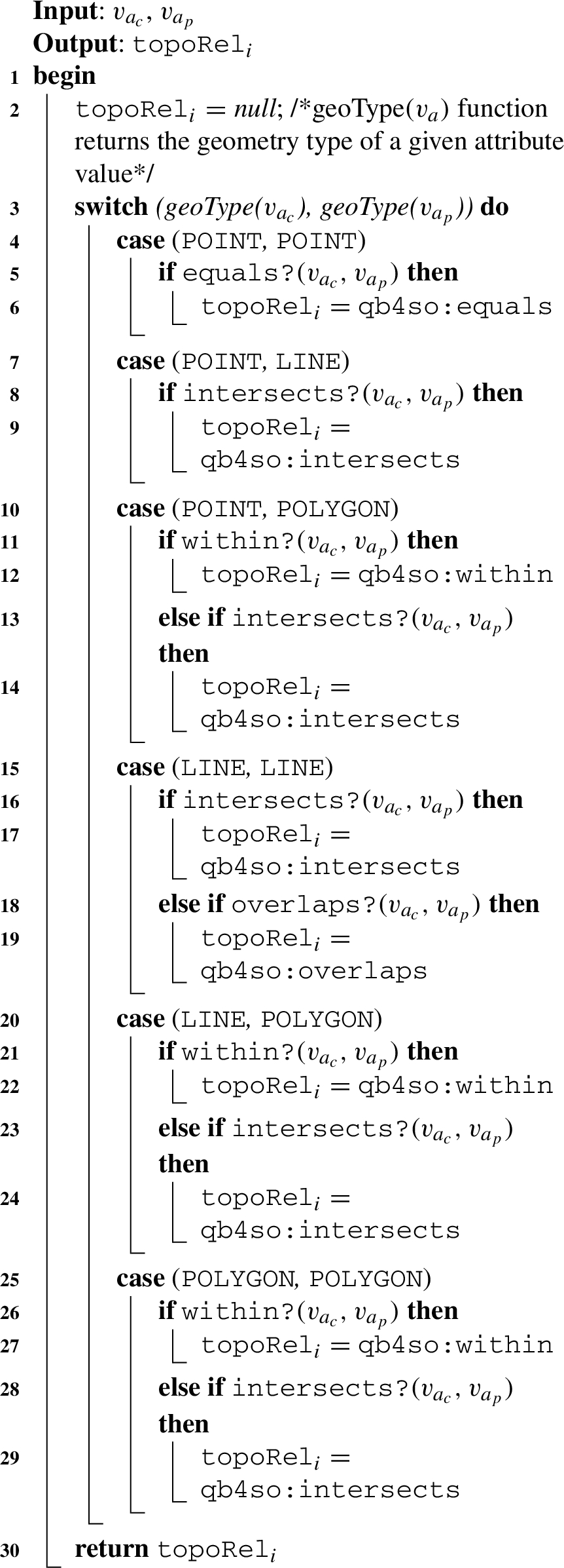
Algorithm 2: (relateSpatialValues) The next helper function is designed based on Table 1, w.r.t. the geometry values of the child-parent level members and based on the structure of a hierarchy step. We prepared Table 1 with topological relations based on DE-9IM.88 We consider only the three simple geometry types, point, line, and polygon as the spatial attribute values of child-parent level members in roll-up relations, excluding complex geometry types, such as multi-polygon, multi-point, etc. The possible topological relations that can occur in a spatial hierarchy step with a roll-up relation from child level to parent level are marked with check sign (✓) in the table. Topological relations, such as contains and covers, are not hierarchically applicable since a spatial child level member cannot contain or cover a spatial parent level member. For these relations, we mark the complete rows with minus sign (−) in the table, since they are not hierarchically applicable. Similarly, we mark the complete columns of line-point, polygon-point, and polygon-line roll-up relations with the minus sign (−) since these are also not hierarchically applicable. This is because we assume that in the instance data, a parent level member should always have a spatial attribute of a geometry type of the same or higher dimensionality of its child level member (a point is 0-dimensional, a line is 1-dimensional and a polygon is 2-dimensional).
Table 1
Topological relations for hierarchy steps (✓: hierarchically and topologically applicable, ×: topologically not applicable, −: hierarchically not applicable)
| Topological relations | Roll-up relations | |||||||||
| Child level | Point (pt.) | Line (ln.) | Polygon (po.) | |||||||
| Parent level | pt. | ln. | po. | pt. | ln. | po. | pt. | ln. | po. | |
| within | × | ✓ | ✓ | − | ✓ | ✓ | − | − | ✓ | |
| contains | − | − | − | − | − | − | − | − | − | |
| intersects | ✓ | ✓ | ✓ | − | ✓ | ✓ | − | − | ✓ | |
| touches | × | × | × | − | ✓ | ✓ | − | − | ✓ | |
| overlaps | × | × | × | − | ✓ | ✓ | − | − | ✓ | |
| crosses | × | × | × | − | ✓ | ✓ | − | − | × | |
| coveredBy | × | × | × | − | × | ✓ | − | − | ✓ | |
| covers | − | − | − | − | − | − | − | − | − | |
| equals | ✓ | × | × | − | ✓ | × | − | − | ✓ | |
For example, a child level member with a spatial attribute of line geometry can only have parent level member(s) with spatial attributes of line or polygon geometries but not point geometry. We mark the topologically not applicable relations with cross sign (×) according to the DE-9IM model (e.g, a line cannot overlap a polygon).
Fig. 8.
Simplifying topological relations.
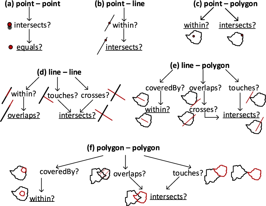
In Fig. 8, we depict the hierarchically and topologically applicable topological relations from Table 1. We simplified them by generalizing the possible relations, e.g., if a line touches or crosses another line at one point, they are both classified as intersects in Fig. 8(d). The most general relations are underlined in Fig. 8 for each pair of geometry types (Fig. 8(a), (b), (c), (d), (e), and (f)).
In Algorithm 2 relateSpatialValues, we only consider these general topological relations that have a higher probability to satisfy the corresponding spatial predicates. For example, the topological relation intersects has the highest probability to satisfy from the DE-9IM matrix [6]. We generalize similar spatial predicates to ones that have higher probability to occur in a 2-dimensional space. For example, relations, such as a line overlaps (along the border of) a polygon, can be generalized to the relation – a line crosses a polygon at a minimum two points, which can later be generalized to the relation – a line intersects a polygon at a (minimum) single point as in Fig. 8(e). Similarly, a line touches a polygon at a single point can be generalized to the relation – a line intersects a polygon at a (minimum) single point.
The topological relation coveredBy requires an area of a geometry, therefore it is applicable only in line-polygon and polygon-polygon relations (Fig. 8(e) and 8(f)). For reasons of simplicity, we choose to generalize them as the within topological relation. In the algorithm, we also prioritize to check the topological relations based on the compared geometry types. If the spatial attribute values to relate are point and polygon geometry types, as in Fig. 8(c), it is more likely that a point is within a polygon than a point intersects a polygon in the instance data.
Therefore, we initially check for a more probable relation in the algorithm. For example, for the point-polygon relations case in Algorithm 2, Line 10: initially, the within spatial predicate is checked in the if statement (Line 11), then the intersects spatial predicate is checked in the else if statement (Line 13). After checking all the possible combinations of spatial attribute values in a switch case, a topological relation is returned from the algorithm (Line 30).
Now that we have introduced spatial helper functions, we present the main algorithms for finding the spatial hierarchy steps in the following.
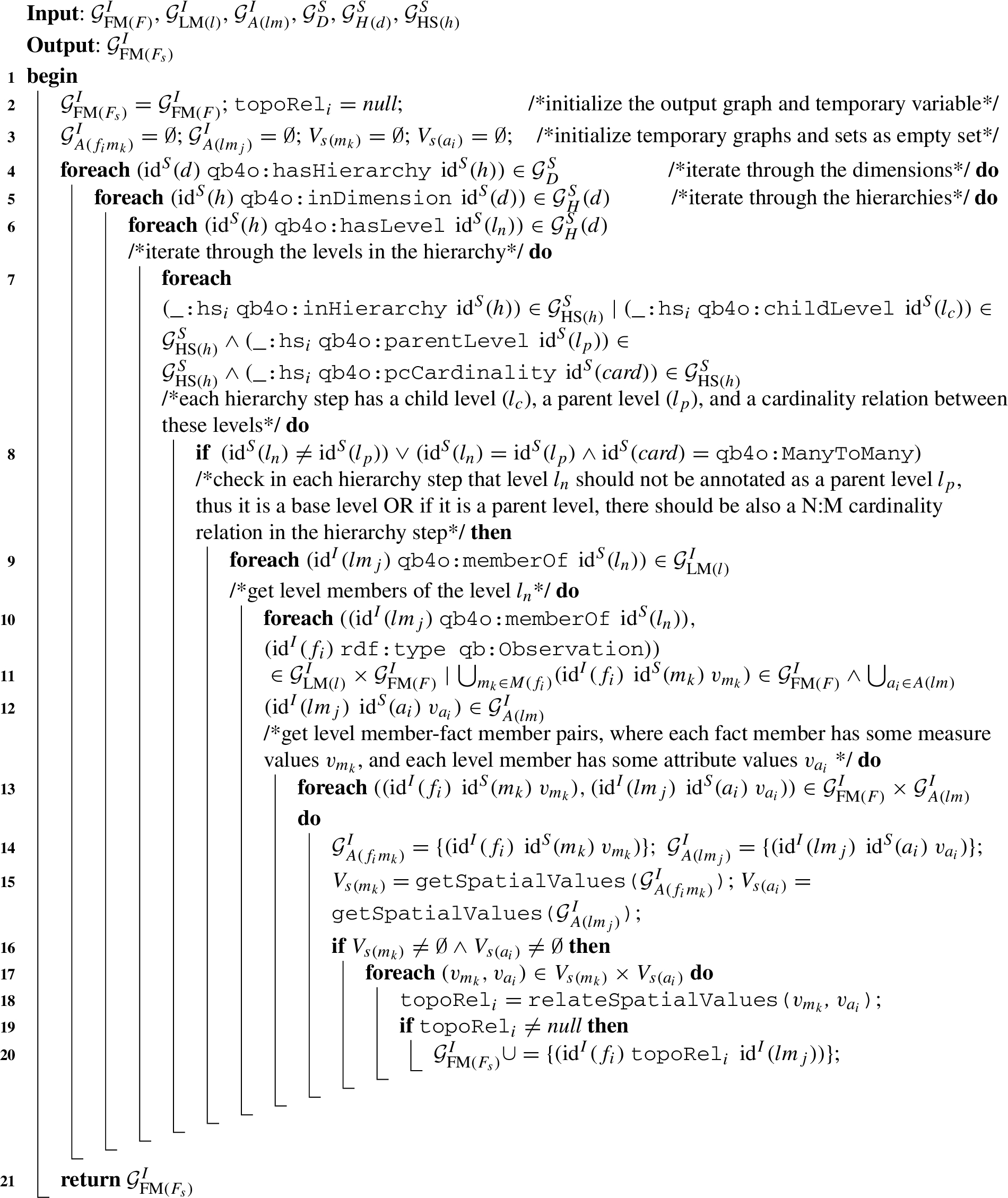
4.1.2.Detecting spatial hierarchy steps
Algorithm 3 (detectSpatialHS) corresponds to case 1 (see the beginning of Section 4.1) and finds the explicit spatial hierarchy steps for QB4OLAP levels with skos:broader roll-up relations between child-parent level members. Intuitively, Algorithm 3 works as follows. Given instance graphs of attributes of level members
As an example, let us consider Listing 2: given Lines 1–6 (
Formally, Algorithm 3 works as follows:
Algorithm 3
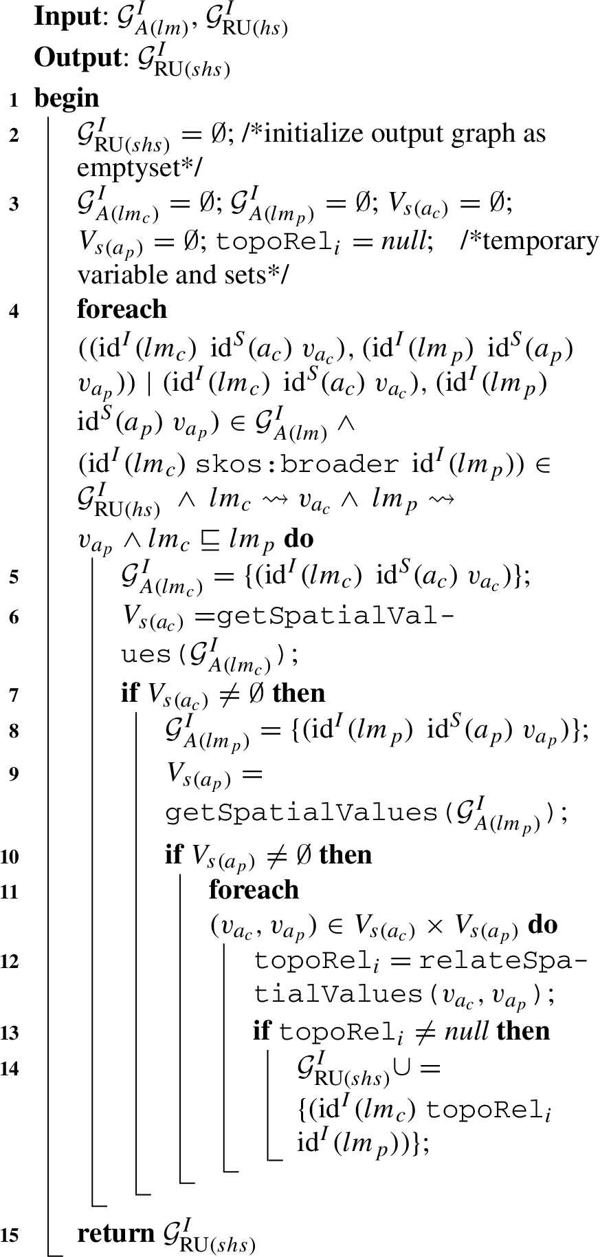
Algorithm 3 (detectspatialHS) The input variables for Algorithm 3 are the instance graphs of attributes of level members
The output of Algorithm 3 is the instance graph of roll-up relations for the detected spatial hierarchy steps
In the foreach loop in Line 4, we go through the elements of the input graphs
In Line 5, while iterating through the foreach loop, we assign the set of triples of child level members and their attributes to the temporary graph
Next in Line 7, if
Similar to Line 6, Line 9 calls the helper function getSpatialValues with the input graph
In this loop, we call the next helper function relateSpatialValues (Algorithm 2), where the input is the spatial value pairs. The output value of this function is the topological relation between the corresponding child and parent level members, and it is assigned to the initially created temporary variable
Finally, the output graph for spatial hierarchy steps
Algorithm 4:
4.1.3.Discovering spatial hierarchy steps
Algorithm 4 (discoverSpatialHS) corresponds to case 2 (see the beginning of Section 4.1) and finds the implicit spatial hierarchy steps for QB4OLAP levels that do not have direct (skos:broader) roll-up relations. In this algorithm, we have to handle the situation where there are no explicit hierarchy steps between level members. Therefore, we benefit from schema graphs capturing dimensions, hierarchies, and levels by iterating through the RDF triples and compare the spatial attribute values of the level members to find the
Intuitively, Algorithm 4 works very much like Algorithm 3, the main difference being that in the absence of a direct link between the members, we need to find it first. Hence, we find pairs of level members exploiting information about dimensions, hierarchies in dimensions, and levels in hierarchies, which is provided by QB4OLAP. The detected pairs are then treated in a similar way as the child-parent level member pairs in Algorithm 3.
As an example, let us consider Listing 2: given Lines 1–6 (
Formally, Algorithm 4 works as follows:
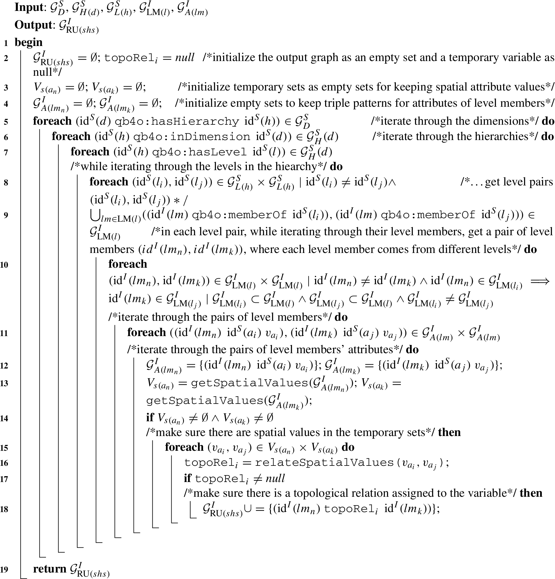
Algorithm 4 (discoverSpatialHS) The input variables for Algorithm 4 are the schema graphs of dimensions
The output of Algorithm 4 is the instance graph of roll-up relations for the discovered spatial hierarchy steps
To discover the spatial hierarchy steps, we need to get the attributes of all the level members from the instance graph (
To achieve that, we use the schema definitions readily available in QB4OLAP, by looping through in Algorithm 4, in nested loops of dimensions in Line 5, hierarchies in the dimension (Line 6), levels in the hierarchy (Line 7). This helps us to determine the levels in a dimension hierarchy, where we can get level pairs from the same hierarchy (Line 8).
Now, while looping through the level pairs, we can identify the level members via the qb4o:memberOf property (Line 9). We get a pair of level members, where each level member should come from a different level, then we iterate through that pair of level members (Line 10).
Then, we get the triple patterns for the attributes of the level members from the each of the level member in the pair, and iterate through those pairs of the triple patterns (Line 11). While iterating through the triple patterns, we insert them to the temporary graphs
Next, we call the helper function getSpatialValues (Algorithm 1) twice, with the input graphs
Then, we iterate through the spatial value pairs retrieved from the each of the sets (Line 15). In this loop, we call the next helper function relateSpatialValues (Algorithm 2), where the input is the spatial value pairs. The output value of this function is the topological relation between the corresponding level members, and it is assigned to the initially created temporary variable
Finally, if this
4.2.Factual enrichment phase
The factual enrichment phase is built around the observation facts and their spatial attributes a.k.a spatial measures and fact-dimension relations (Section 2.1).
Listing 3.
GeoFarmHerdState fact schema definition in QB4SOLAP
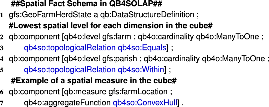
In QB4OLAP facts are linked to the dimensions at the lowest granularity level, which is the base level of the dimensions. For example, the GeoFarmHerdState cube has two spatial base levels linked to the cube: Parish level and Farm level. The GeoFarmHerdState cube also has a spatial measure listed in the cube: FarmLocation (Fig. 3). In QB4OLAP, a fact schema defines the structure of a cube with the qb:DataStructureDefinition property (Listing 3, Line 1). Base levels (Lines 2 and 4) and measures (Line 6) are given as qb:components of the fact (Listing 3). The cardinality relationship between the base level and the fact can also be represented with qb4o:cardinality in QB4OLAP as given in Lines 2 and 4 in Listing 3.
On the other hand, with QB4SOLAP we can also represent fact-level topological relations that are similar to the topological relations between the child-parent levels at the hierarchy steps. Fact-level topological relations are given in spatial fact schema with blue in Lines 3 and 5 (Listing 3). QB4SOLAP also extends the (cube) schema with spatial aggregate functions, which are defined over spatial measures as highlighted in blue (Listing 3, Line 7).
Listing 4.
GeoFarmHerdState fact member with base levels and measures
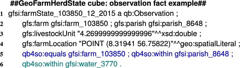
An example of an observation fact (fact member) at the instance level is given in Listing 4. A fact member is a qb:Observation (Line 1), which is related to the base levels (Line 2) with respect to the data structure definition (DSD) of the fact schema, and has a set of measures (Lines 3, 4) where some measures (Line 4) might have spatial values (Listing 4). To define a QB4OLAP fact schema, first, we need to enrich the fact members by annotating with topological relations as highlighted with blue in Line 5. We can derive topological relations between fact members and the (base) level members by comparing the spatial measures of the fact members and spatial attributes of the (base) level members with Boolean spatial predicates. The links between fact members and base level members are already given explicitly in Line 2 (Listing 4). However, these links are simple references between the fact and base level members, which do not describe the nature of the topological relation. By applying Boolean spatial predicates on fact and level members, we can find the exact topological relations, i.e., if a fact member intersects with the level member or if a fact member is within the level member. We explain how to detect these explicit fact-level (topological) relations in Section 4.2.1.
Moreover, there might also be some missing links between the (observartions) fact members and the corresponding base level members. For this case we need to find all the base level members that are spatial and derive the links between the spatial measure values and spatial attribute values (of the base level members) by using Boolean spatial predicates. We explain how to discover fact-level (topological) relations, which are not explicitly linked between observation fact and base level members in Section 4.2.2.
There are also cases where we would like to establish a direct (topological) relation between the fact members and higher granularity (parent) level members, which are not at the base level of the dimension. Using the example depicted in Fig. 4 we explained that wrongly aggregating the measures (i.e., double counting) becomes a problem when we roll-up between the levels that have many-to-many (N:M) cardinality relations (as in Parish and Drainage Area levels). Therefore, it is necessary to drill-down to the lowest granularity (fact members) and find the direct relation between the observation fact members and the corresponding level members of the higher level in many-to-many cardinality relations.
In order to prevent this problem, we address the issue in our algorithm to discover and annotate the fact-level (topological) relations that are between the observation fact members and level members of a higher level in an N:M cardinality relation in Section 4.2.2. For example, such a relation is given in green in Line 6 (Listing 4) that shows a topological relation between an observation fact member (farm state) and a higher level – not a base level – member (drainage area).
Finally, in Section 4.2.3 we explain how to define a data structure definition (DSD) of spatial fact schema using a QB4OLAP fact schema and the spatial fact member instances derived in the previous two algorithms.
4.2.1.Detecting explicit fact-level relations
In this section, we present an algorithm for detecting explicit fact-level topological relations between observation fact members and base level members where there is a direct reference between the fact member and the base level member. To derive these topological relations we need to get the spatial attributes of fact members (spatial measures) and base level members.
Algorithm 5
Algorithm 5 (detectFactLevelRelations) The input variables for Algorithm 5 are the instance graphs of fact members
Every fact member
The output of Algorithm 5 is the enriched instance graph of fact members with topological relations
In the first foreach loop (Line 4 and 5) we retrieve the observation fact members from the input graph of fact members, which corresponds to Line 1 in Listing 4. Getting the fact members allows us to access each of their measures in Line 6 and level members in Line 7 (Algorithm 5). In the next foreach loop (Line 9) we match each measure-level member pair, where we can already retrieve the measure values from the input graph of fact members
Algorithm 6:
4.2.2.Discovering implicit fact-level relations
In this section, we present an algorithm for discovering fact-level (topological) relations, where there are no direct links between the fact and level members. This algorithm handles the following situations: 1) Finding the topological relations between observation facts and base level members; 2) Finding the topological relations between observation facts and parent level members in an N:M cardinality relation. In both cases there are no direct links between the observation facts and level members. Therefore, we benefit from (QB4OLAP) schema graphs of dimensions, hierarchies, and levels for iterating through the RDF triples to distinguish the base level members, and find the parent level members, when there is an N:M cardinality relation between the levels of a hierarchy at a hierarchy step.
Algorithm 6 (discoverFactLevelRelations) The input variables at the schema level for Algorithm 6 are the schema graphs of dimensions
The input variables at the instance level are the instance graphs of fact members
The output of Algorithm 6 is the enriched instance graph of fact members with the topological relations
To find the topological relations between observation facts (with spatial measures) and base level members (with spatial attributes), first, we need to find all the base levels since there is no direct link between the fact and level members. To achieve this in Algorithm 6, we use the schema definitions readily available in QB4OLAP. In Line 4, we iterate through the nested loops of dimensions to get the hierarchies and in Line 5 we iterate the nested loops of hierarchies to get the hierarchy levels. To find the base level of a hierarchy, we have to iterate through the hierarchy steps, where each hierarchy step describes a child level, a parent level and a cardinality relation between the levels (Line 6). If a level
Thus, we can retrieve the level members of level
Then, in the next foreach loop in Line 12, we get the triple patterns with each measure values of the fact member and attribute values of the level member in pairs. While iterating through the (pair of) triple patterns, we insert each member of the pair to the temporary graphs for measures of fact members
Then, we iterate through the spatial value pairs retrieved from the each of the sets (Line 16). In this loop, we call the next helper function relateSpatialValues (Algorithm 2), where the input is a spatial value pair. The output value of this function is the topological relation between the corresponding level members, and it is assigned to the initially created temporary variable
To find the topological relations between the observation facts and parent level members in an N:M cardinality relation, we check in Line 20 that if level
Finally, the output graph for the spatial fact members with discovered fact-level (topological) relations is returned in Line 22.
4.2.3.Defining spatial fact DSD
In this section, we present an algorithm for re-defining the fact schema data structure definition (DSD) by enriching the DSD with fact-level topological relations. An example of a fact schema in QB4OLAP is given in the black-colored lines of Listing 3 (for now please ignore Lines 3, 5 and 7). We re-define the spatial fact schema to QB4SOLAP (Listing 3 Lines 1–7) by using the enriched fact members that are generated via Algorithms 5 and 6.
Algorithm 7:
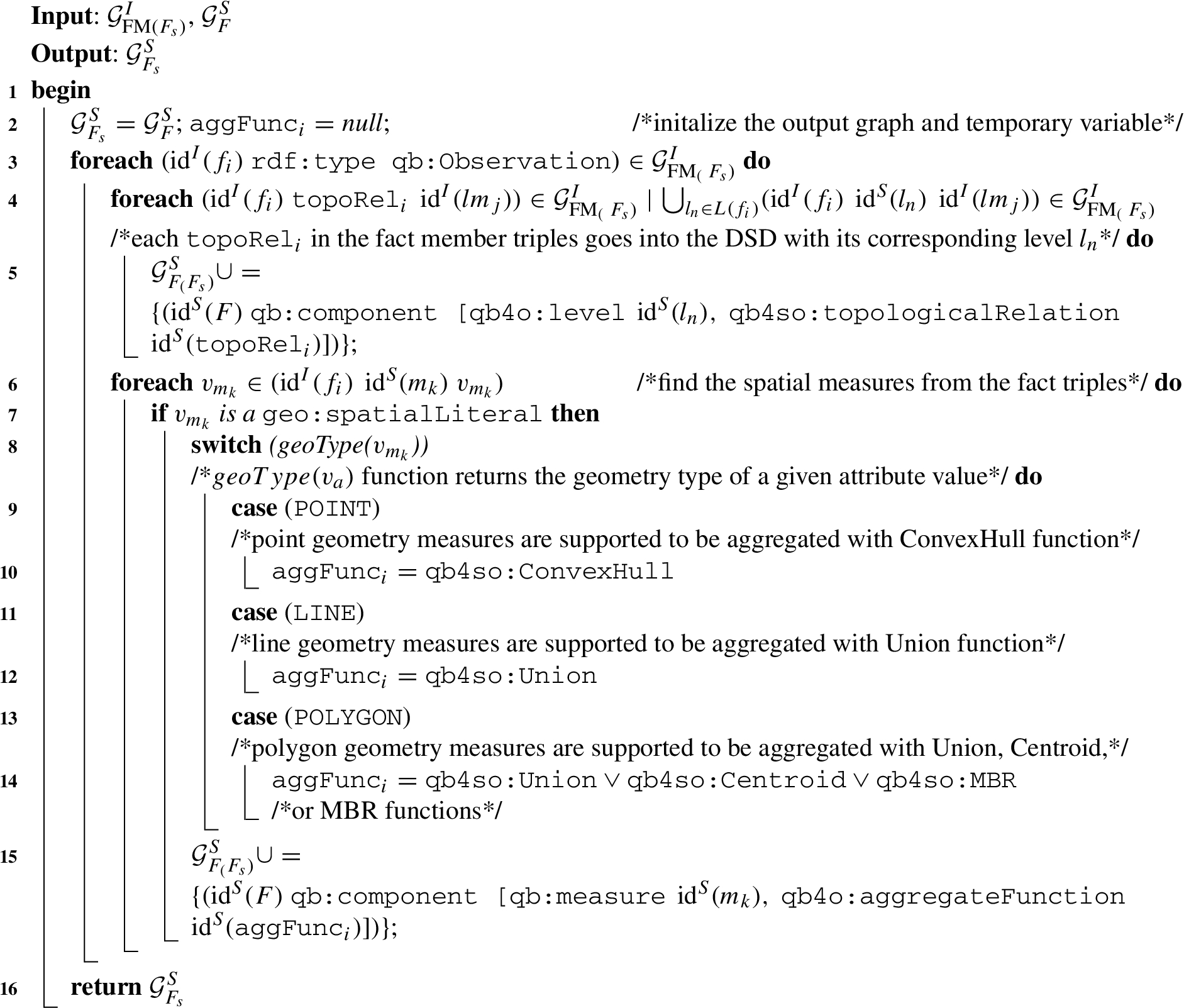
Algorithm 7 (defineSpatialFactDSD) The input variables for Algorithm 7 are the instance graph of spatial fact members
The output of Algorithm 7 is the enriched fact schema graph
In Line 2, we initialize the output graph as the input schema graph so that we can gradually enrich it with QB4SOLAP schema annotations (Lines 5 and 15). Initially, an aggregate function variable
The first foreach loop iterates through the fact members graph
4.3.Implementation choices
When implementing the algorithms presented in this section, we had to make some implementation choices both in technical as well as strategical aspects that we would like to briefly comment on. Further details regarding the implementation of the algorithms themselves are available in the Appendix. As mentioned earlier, RDF2SOLAP is implemented in Javascript on the Node.js platform using the N3.js library for parsing the RDF triples in Javascript and the Turfjs library for spatial analysis. Details of our approach, endpoints, and datasets can be found on our project page.1212 The code repository for the whole implementation can be found on GitHub.1313
To answer the question: “Can this approach be reasonably implemented on top of triple stores by directly using Web and Semantic Web technologies?”, we have come across a number of challenges, where specific choices had to be made.
For example, we chose to store RDF data in a well-established triple store (Virtuoso Open Source) that supports many geometry data types (i.e., POLYGON, MULTIPOLYGON). Even though Virtuoso supports several shape types (e.g., POLYGON, MULTIPOLYGON, etc.), it has a limited number of spatial Boolean functions available as built-in functions from the DE9DIM model (see Table 1). Therefore, we have also decided to use a third party Javascript library for spatial analysis, which is called Turfjs6. This way, we can ensure that RDF2SOLAP can be used on top of any triple store since the Javascript library provides us with the spatial analysis capabilities and a flexible development environment, independent from the choice of the triple store.
We are working with multi-part POLYGON data (for drainage areas and parishes), which means that, when several polygons are grouped by unique (parish or water) URIs they can compose a MULTIPOLYGON for a single parish or drainage area instance. From the implementation point of view, we had to implement a bounding box function for multi-part POLYGON data, in order to call the spatial Boolean functions (within and intersects) between the correct parish and drainage area instances, then annotate the topological relations between their unique URIs. If triple stores already provided overall support of complex spatial data types, spatial indices, and a complete support of built-in spatial functions, decoupling the triple stores during development of RDF2SOLAP would not have been necessary. We could then directly have used the spatial capabilities of the triple stores that were required for developing RDF2SOLAP. However, to the best of our knowledge, a third party spatial analysis library was needed to fully implement our RDF2SOLAP (spatial) multi-dimensional enrichment algorithms described in Section 4.
5.Experimental evaluation
The section is structured as follows. We describe experimental settings in Section 5.1. Then we compare development time between our approach and the baseline, followed by a comparison of the runtimes and the annotation quality. Finally, we summarize our findings in Section 5.5.
5.1.Experimental setup
The rationale for developing RDF2SOLAP is to be able to enrich and annotate existing spatial RDF data with spatial and multi-dimensional metadata while staying within the RDF environment. This upgrades the spatial RDF data to allow SOLAP querying directly in SPARQL. The alternative would be to export the spatial RDF data to relational format, do the enrichment with relational/GIS tools and perform the SOLAP on the resulting relational data, thus loosing all the advantages of having the data in RDF in the first place. Doing the enrichment purely within the RDF environment is expected to come at a cost as support for spatial and multidimensional data in the RDF/SW stack is still less mature; this will however improve over time. Thus, our goal is just to demonstrate that we can do this in a pure RDF environment with adequate performance in terms of runtime and annotation quality (which may vary). In return, RDF2SOLAP provides a solution that is both flexible and general for all data sets. We then compare our general solution to the alternative baseline, which is spending long development times on hand-crafting specialized enrichment solutions using RDBMSes and GIS for each new data set.
We used the common Virtuoso version 07.20.3217 on Linux (x86_64-ubuntu-linux-gnu), Single Server Edition as triplestore. We implemented RDF2SOLAP on the Node.js platform, running on a Macbook Pro 14.3 with one Intel Core i7 2.8GHz 4-core CPU 256KB L2 cache, 6MB L3 cache, and 16GB RAM. All test cases are in the GitHub repository so the experiments can be repeated. Each experiment was run in a single process. For the baseline implementation, we used a leading GIS tool and a leading RDBMS (we cannot write the names due to license restrictions, but they can be supplied on demand). These were running on a Windows 10 Enterprise server with 4 Intel Core i7 2.9GHz CPUs and 32GB memory, i.e., considerably more powerful hardware. We use both the GeoFarmHerdState data set described above and the GeoNorthwind data set from [15].
We now describe how the RDBMS and GIS baselines were implemented. Since the GIS tool and the RDBMS cannot process RDF data in native format, we first have to extract and prepare the data for loading into them. The preparation time is part of the development time discussed below. Doing this preparation requires that the developer has basic knowledge of the domain, extraction of RDF data with SPARQL queries, writing SQL queries, and knows how to use the RDBMS and GIS tools. We extracted the spatial level members (farms states, parishes, and drainage areas) from our RDF endpoint in CSV format. To load the data into the GIS tool and RDBMS we use the relational schema defined by QB4SOLAP. In the GIS tool we saved CSV data layers (for each level; farm states, parishes and drainage areas) and converted these into native GIS format (shape files). Then, we run the Join Attributes By Location function, which is a built-in data management function. We run this function as a batch process, for parishes-drainage areas (Alg. 4), farm states-parishes, and farm states-drainage areas (Alg. 6). We load the WKT data (spatial attributes of level and fact members) in the CSV files into the GIS tool and a relational geo-database, with the same decimal precision for the coordinates. We extract topological relations between the child and parent members by using spatial joins in the GIS tool and built-in spatial functions in the RDBMS. Overall, most of the time was spent on data extraction, preparation, and load, caused by having to convert data from its existing RDF format. None of these tasks are needed if the enrichment is done entirely within an RDF environment, like in RDF2SOLAP.
5.2.Development time comparison
We now compare the time required to develop enrichment solutions for spatial RDF data with RDF2SOLAP to using the RDBMS and GIS baselines. Here, it is important to keep in mind that RDF2SOLAP has general algorithms that use existing metadata and annotations to work for any spatial RDF data set, requiring only a few minutes of configuration, while a new baseline enrichment solution has to be implemented for each new data set, requiring literally (repeated) days of development time. Of course, there was a onetime development cost for RDF2SOLAP. However, this cost is already paid and will not be repeated, unlike the case for the baselines.
The development times for RDF2SOLAP, and the RDBMS and GIS baselines for the one-time step of General Algorithms (only RDF2SOLAP) and the GeoFarmHerdState data set, are given in Table 2. One day corresponds to 8 hours. All development was carried out by the first and fourth author who both have significant experience in all the used tools and platforms, and also recorded the development times for RDF2SOLAP and GeoFarmHerdState. The RDF2SOLAP configuration times for each data set were also recorded by the first author. We find these development times realistic and comparable. As GeoNorthWind is only included to demonstrate that RDF2SOLAP can generalize to other data sets, we have not implemented the baseline enrichment solutions for GeoNorthWind. Thus, we have not reported RDBMS and GIS development times in the table. However, realistic estimates would be in the same range as for GeoFarmHerdState, i.e., one or more days.
Table 2
Development times
| RDF2SOLAP | RDBMS | GIS | |
| General algorithms | 1.4 days (one-time) | N/A | N/A |
| GeoFarmHerdState | 5 min (config) | 1.3 days | 2 days |
| GeoNorthWind | 10 min (config) | N/A | N/A |
Table 3
Input, output, and runtimes for RDF2SOLAP algorithms on GeoFarmHerdState
| INPUT | OUTPUT | ||||||
| NumberOf child members | NumberOf parent members | NumberOf explicit relations | NumberOf topological relations | Run times (in seconds) | |||
| Section 5.2 | Alg. 3 | parishes: 2,180 | drainageAreas: 134 | 2,683 | intersects | 636 | 29 s |
| within | 2,046 | ||||||
| Alg. 5 | farmStates: 40,039 | parishes: 2,180 | 39,800 | within | 39,334 | 7 s | |
| Section 5.3 | Alg. 4 | parishes: 2,180 | drainageAreas: 134 | NONE | intersects | 1,088 | 2,622 s |
| within | 3,392 | ||||||
| Alg. 6 | farmStates: 40,039 | parishes: 2,180 | NONE | within | 39,998 | 1,920 s | |
| farmStates: 40,039 | drainageAreas: 134 | NONE | within | 39,845 | 525 s | ||
From the table, we can see that RDF2SOLAP allows to enrich and annotate new spatial RDF data sets with just minutes of effort, since the enrichment process is done automatically after retrieving the input parameters to the enrichment algorithms from the endpoint. In comparison, each new data set requires one or more days of (repeated) development effort for the baseline RDBMS and GIS enrichments.
5.3.Runtime comparison
Having established that RDF2SOLAP requires up to 2 orders of magnitude less development time for a new data set, we now investigate whether it can do the enrichment with reasonable runtimes, and compare its runtimes to those of the baseline implementations. Both the total runtimes (in minutes) and the subtotals (in seconds, for accuracy) for the different algorithms are reported. The GeoFarmHerdState runtimes are seen in Tables 3 and 4.
Alg. 3 and 5 (to detect explicit topological relations) are only implemented in the RDBMS since the GIS tool does not support the foreign key joins of explicit (skos:broader) relations which are needed for these two algorithms. In order to implement the needed topological relations in RDF2SOLAP, we had to use theturf.js library running on a node.js server, where the RDF data is parsed into JSON format, since these relations were not supported by the triplestore. This meant that we could not take advantage of spatial indexing in the triplestore.
To understand the size of the input and output of the algorithms for GeoFarmHerdState, we report these along with corresponding RDF2SOLAP runtimes in Table 3. The input parameters and numbers for each algorithm are shown in Table 3 under the INPUT column(s). The input datasets to the algorithms are 2,180 parish members, 40,039 farm state members, and 134 drainage area members. The OUTPUT columns show the number of topological relations found and run times of the algorithms. In this section, we only focus on the runtime, the annotation quality is evaluated later.
Table 4
GeoFarmHerdState runtimes (f.s. = farm states, p. = parishes, d.a. = drainage areas)
| RDF2SOLAP | RDBMS | GIS | |
| Alg. 3 (p. – d.a.) | 29 s | <1 s | N/A |
| Alg. 4 (p. – d.a.) | 2,622 s | 43 s | 45 s |
| Alg. 5 (f.s. – p.) | 7 s | <1 s | N/A |
| Alg. 6 (f.s. – p.) | 1,920 s | 95 s | 72 s |
| Alg. 6 (f.s. – d.a.) | 525 s | 48 s | 41 s |
| Total | 85 m | 3 m |
In Table 3, we can see that most expensive algorithm is Alg. 4 (discoverSpatialHS), which runs in 2,622 seconds. The algorithm takes parishes and drainage areas (POLYGON data type) as input instances, and not explicit relations as in Alg. 3 (detecSpatialHS). Alg. 3, given (2,683) distinct explicit relations, checks the corresponding spatial Boolean functions (within and intersects) 2,683 times each. In comparison, Alg. 4 calls (within and intersects) 134 × 2,180 = 292,120 times each. Similarly, Alg. 6 is slower than Alg. 5 since the former does not use explicit relations. However, it is much faster than Alg. 4 since this calls the spatial Boolean functions between farm states (POINT data type) and parishes and drainage areas (POLYGON data type).
From the GeoFarmHerdState runtimes, we see that Alg. 4 and 6 use the most time, in particular for RDF2SOLAP. However, the total RDF2SOLAP runtime of 85 minutes is very reasonable and well within the requirements for practical use: a user wanting to analyze a new data set (which usually does not happen several times a day) can simply spend a few minutes on configuration and then let RDF2SOLAP run in the background for the next 1.5 hours. Especially for non-developer RDF users, this is a much better value proposition than first spending one or more days on technical development in the baseline tools.
For GeoNorthWind, the baselines were not implemented (see above) so only RDF2SOLAP runtimes are reported, see Table 5. For this smaller data set, RDF2SOLAP completes in just 26 seconds, making it usable even in interactive mode.
Table 5
GeoNorthWind runtimes
| Hierarchy step | Algorithm | RDF2SOLAP |
| Customer-city (point-polygon) | Alg. 3 | 2 s |
| Alg. 4 | 7 s | |
| Supplier-city (point-polygon) | Alg. 3 | <1 s |
| Alg. 4 | <2 s | |
| City-state (polygon-polygon) | Alg. 3 | 1 s |
| Alg. 4 | 13 s | |
| Total | 26 s |
In summary, the runtime comparisons show that, even though RDF2SOLAP is slower than the hand-crafted baselines, it still has a runtime performance that is more than adequate for its intended use case.
5.4.Annotation quality comparison
We now compare RDF2SOLAP to the RDBMS and GIS baseline tools in terms of annotation quality. Specifically, we report the number of the topological relations found by each algorithm/step in each tool, and relate these to accuracy and coverage. The numbers are given in Table 6.
Table 6
Number of topological relations found by each tool (f.s. = farm states, p. = parishes, d.a. = drainage areas)
| Tools | ||||
| GIS | RDBMS | RDF2SOLAP | ||
| Alg. 3: (p. – d.a.) | intersects | N/A | 1,897 | 636 |
| within | N/A | 785 | 2,046 | |
| Alg. 4: (p. – d.a.) | intersects | 2,556 | 2,802 | 1,088 |
| within | 1,039 | 785 | 3,392 | |
| Alg. 5: (f.s. – p.) | within | N/A | 39,334 | 39,334 |
| Alg. 6: (f.s. – p.) | within | 39,805 | 39,984 | 39,998 |
| Alg. 6: (f.s. – d.a.) | within | 39,441 | 39,845 | 39,845 |
As mentioned earlier, Alg. 3 and Alg. 5 were not implemented in the GIS tool due to its lack of support for explicit relations between parent-child members; thus these numbers are reported as N/A. We thus only tested the discovery of implicit topological relations (discoverSpatialHS and discoverFactLevelRelations) by utilizing its spatial join functionality to emulate the results for Alg. 4 and Alg. 6.
For the RDBMS tool, we tested both detect and discover topological relations, where we used joins on unique IDs if they were present (drainage area foreign key in parishes, parish foreign key in farm states), and with spatial joins by using the STWithin, STIntersects, and STOverlaps built-in functions.
We now compare results for each algorithm in the different tools. For Alg. 3, RDF2SOLAP reports only a third of the intersecs relations but almost three times as many within relations, as the RDBMS tool. This is due to generalizing the multi-part POLYGON data as bounding boxes in RDF2SOLAP (due to restrictions in our spatial library), in the spatial RDBMS, multi-part POLYGON data is processed in its original format, yielding better quality. Interestingly, the total number of intersects+within relations for the two tools are exactly the same, namely 2682. This suggest that RDF2SOLAP can get the same annotation quality as the RDBMS tool when better spatial support become available in the RDF environment.
Similar results are seen for Alg. 4. Here, the GIS and RDBMS results are similar, but not identical, showing that perfect annotation quality is not a given, even with traditional tools. Again, RDF2SOLAP finds fever intersects relations and more within relations (again due to the bounding box generalization), and again the total number of relations found by the 3 tools are very similar. This indicates that RDF2SOLAP can achieve the same annotation quality with better spatial RDF support.
For Alg. 5, the RDF2SOLAP and RDBMS results are identical. This perfect annotation quality can be achieved since the within relations are found between points and polygons which can be done exactly by the library.
For Alg. 6, the results found by the 3 tools for (farm states-parishes) are very close, with RDF2SOLAP differing 0.5% from the GIS tool and 0.04% from the RDBMS tool. For (farm states-drainage areas), the RDF2SOLAP and RDBMS results are identical, while the GIS result differs by 0.01%. Thus, the annotation quality for all 3 tools is near-perfect.
Similar results were found for GeoNorthWind. For Hierarchy Step 1, there are 89 correct within relations. Of these, Alg. 3 found 75 of them correctly, while Alg. 4 found 91 relations (the 89 correct and 2 extra incorrect). For Hierarchy Step 2 there are 28 correct within relations: Alg. 3 found 24 of them correctly, while Alg. 4 found all 28 of them correctly. For Hierarchy Step 3, we do not have the correct ground truth since this requires the GIS and RDBMS baselines to have been implemented.
RDF2SOLAP’s problems with POLYGON-POLYGON relations could have been prevented if we had been able to use multi-part POLYGON and MULTIPOLYGON data in its original form instead of generalizing them to bounding boxes. However, We encountered both performance and formatting problems while loading MULTIPOLYGON data to Virtuoso, which led to missing data in the triplestore for drainage areas. Even if the MULTIPOLYGON data was could be successfully loaded, Turf.js is not able to handle POLYGON-MULTIPOLYGON within relations. We thus had to make a trade-off and implement the POLYGON-POLYGON relations with generalized bounding boxes.
In summary, the annotation quality of RDF2SOLAP is near-perfect for the spatial relations that are well supported in the RDF environment. There are some problems with polygon-to-polygon relations, but these are caused by limitations in our spatial library. When better spatial RDF support becomes available, we are confident that RDF2SOLAP will provide near-perfect annotation quality for all cases.
5.5.Experimental summary
In summary, we have seen that RDF2SOLAP provides orders of magnitude less development time for new data sets (minutes versus days), and, while slower than the RDBMS and GIS tools, has adequate runtimes for its intended use case. For some algorithms, its annotation quality is near-perfect, while for others, it will be when better spatial RDF support becomes available.
6.Related work
Utilizing DW/OLAP technologies on the Semantic Web with RDF data makes RDF data sources more easily available for interactive analysis. As summarized by Abelló et al. [1], related work has studied OLAP and data warehousing possibilities on the Semantic Web (SW) in general. Our work, however, is centered around spatial OLAP (SOLAP) and spatial data warehouses (SDW) on the Semantic Web, which is not yet a comprehensively studied research topic. We focus on performing spatial OLAP analysis directly over multi-dimensional data published on the Semantic Web. Therefore, we review the related work with relevant approaches classified under the following titles: (1) data modeling and representation (on the SW for multi-dimensional and spatial data), (2) metadata enrichment and MD analysis (OLAP-like analysis over RDF data).
Data modeling and representation The RDF Data Cube (QB) vocabulary [48] is the W3C recommendation to publish statistical data and its metadata in RDF. Thus, QB is commonly used to publish raw or already aggregated multidimensional data sets. However, QB lacks the underlying metadata for multidimensional models and OLAP operations. The set of MD concepts, such as, hierarchy levels along a cube dimension, semantics of the relationships between levels, semantics and definitions of aggregate functions are missing in QB vocabulary, are essential in an MD schema to enable OLAP analysis. Therefore, Kämpgen et al. define an OLAP data model on top of QB by using SKOS [30] extensions1414 to support multi-dimensional hierarchies [26,27]. However, the proposed model has some limitations on levels to exist only in one hierarchy. The OLAP operations are made available on the data cubes with the proposed model but restricting the cubes with only one hierarchy per dimension. Etcheverry et al. propose QB4OLAP [7] as an extension to the QB vocabulary, which supports modeling a complete MD data cube and querying the cube with OLAP operations on the Semantic Web. Modeling of MD data on the Semantic Web motivated the publication of datasets from several domains (e.g., statistical data sets from EuroStat and World Bank data, AirBase air quality data, and many other environmental and governmental open data) as RDF data cubes [47].
The need of fully multi-dimensional semantic data warehouses (where OLAP operations are enabled in SPARQL) made the QB4OLAP vocabulary prominent. Therefore, RDF data cubes from statistical and environmental domains [10,12,43] are published with an extended QB vocabulary. Moreover, semantic Extract-Transform-Load (ETL) tools automate and ease the process of annotating and publishing open data with QB4OLAP on the Semantic Web [5,31,32]. Therefore, we can see more and more multi-dimensional datasets annotated with QB4OLAP on the Semantic Web.
These multi-dimensional semantic modeling approaches and querying with OLAP on the Semantic Web lead us to find ways for modeling, publishing, and querying spatial data warehouses in particular since modeling and querying spatial data bring new challenges. QB4SOLAP [13] – a spatial extension to a fully multi-dimensional QB4OLAP vocabulary emerges the need of modeling and publishing geo-semantic data warehouses on the Semantic Web.
Modeling and publishing (non multi-dimensional) spatial data on the Semantic Web has been a focus by many communities and research groups. Some of the efforts for standardizing and aligning vocabularies to describe spatial data (e.g., locations, geometries, etc.) are GeoSPARQL [34] by the Open Geospatial Consortium (OGC), Basic Geo (WGS84 lat/long) Vocabulary by W3C Semantic Web Interest Group [4], NeoGeo Vocabularies by GeoVocab working group [40], INSPIRE Directive metadata on the Semantic Web [35], and GeoNames Ontology [45] among many others.
These standards have been commonly used in a wide range of projects. Government Linked Data (GLD) working group listed some of these geo-vocabularies as standards to publish governmental linked data sets [20]. Andersen et al. re-use some of these vocabularies for publishing governmental and spatial data on the Semantic Web [2]. LinkedGeoData is a big contribution to the Semantic Web, which interactively transforms OpenStreetMap data to RDF data [41]. The GeoKnow project focuses on linking geospatial data from heterogeneous sources [39]. More recent works by Kyzirakos et al. to transform geospatial data into RDF graphs using R2RML mappings [28] and geo-semantic labelling of open data [33] by Neumaier et al. show that spatial data on the Semantic Web will keep growing. However, none of these standards considers the MD aspects of spatial data for geo-semantic data warehouses.
Large volumes of spatial data on the Semantic Web yield a need for advanced modeling and analysis of such data. As mentioned earlier, QB4SOLAP [13] remedies this need. Aggregate functions, cardinality relationships, and topological relations are rich sources of knowledge in spatial data cubes in order to query with spatial OLAP operations in SPARQL [15].
QB4ST [3] is a recent attempt to define extensions for spatio-temporal components to RDF Data Cube (QB). However, it has the inherent limitations of QB to support OLAP dimensions with hierarchies, levels, and aggregate functions. Lack of OLAP hierarchies and aggregate functions in QB4ST hinders to define and operate with topological relations at hierarchy steps or spatial aggregate functions on spatial measures, which are essential MD concepts for SOLAP operators. These spatial MD concepts in geo-semantic data warehouses are defined together with SOLAP to SPARQL query mappings in [15].
Metadata enrichment and MD analysis Increasing popularity of RDF data cubes and MD OLAP cubes on the Semantic Web raised interest in tools and frameworks that can ease the annotation and querying of MD data on the Semantic Web from existing RDF sources.
Ibragimov et al. present a framework for exploratory OLAP over Linked Open Data (LOD), where the MD schema of the data cube is annotated with QB4OLAP [22]. Based on this MD schema, they propose a system that is capable of querying data sources, extracting and aggregating data to build OLAP cubes in RDF [23] and querying in a federated setup [21]. Similarly, Gallinucci et al. propose an exploratory OLAP approach, namely iMOLD by interactively MD modeling of linked data [11]. Their approach allows users to enrich RDF cubes with aggregation hierarchies through a user-guided process. During this interactive process, the recurring modeling patterns that express roll-up relationships between RDF concepts are recognized in the LOD, then these patterns are translated into aggregation hierarchies to enrich the RDF cube. Varga et al. enables OLAP analysis with the QB2OLAP tool in [43] over statistical data published with QB vocabulary, by applying dimensional enrichment steps described thoroughly in [44]. The proposed enrichment steps allow users to enrich a QB dataset with QB4OLAP concepts such as fully-fledged dimension hierarchies. However, none of these frameworks and approaches supports spatial data warehouses and SOLAP operations.
In this paper, we propose a framework, where OLAP cubes in RDF can be enriched with spatial MD concepts from the QB4SOLAP vocabulary by employing RDF2SOLAP enrichment algorithms over QB4OLAP triples. This allows users to query MD cubes with SOLAP operators in SPARQL. Optionally, users can utilize GeoSemOLAP [14] tool on top of QB4SOLAP data sets, which helps users formulate SOLAP queries in SPARQL.
7.Conclusion and future work
Motivated by the need to conciliate MD/OLAP RDF data cubes and spatial data on the Semantic Web as geo-semantic data warehouses, we have presented a number of contributions in this paper. As a first attempt to enrich RDF data cubes with spatial concepts, we have shown that the QB4SOLAP vocabulary yields the need for fully-fledged spatial data warehouse concepts (that is built on top of non-spatial QB4OLAP and RDF Data Cube (QB) vocabularies), by demonstrating the running use case examples from real world governmental open data sets from various domains (i.e., environment, farming) with complex geometry types. We introduced running use case examples annotated both with QB4OLAP and QB4SOLAP vocabularies, in RDF triples and formalized the RDF triples as parameters to use in the enrichment algorithms. Second, we have built our conceptual architecture in relation to existing semantic (spatial) OLAP tools (e.g., on top of the QB2OLAPem enrichment module and at the back-end of GeoSemOLAP). Third, we have provided hierarchical enrichment algorithms for two cases that cover finding explicit hierarchy steps with direct links between the level members and finding implicit hierarchy steps (without direct links between the level members) by comparing geometry attributes of the level members. We have defined and deployed the necessary algorithms as spatial helper functions for finding spatial attributes and comparing these attributes to derive topological relations. Fourth, we have presented the factual enrichment phase for both implicit and explicit fact-level relations between the fact and level members. Moreover, we have presented how to re-define the fact schema after the factual enrichment phase in an automated manner. Re-defining the fact schema also includes finding the spatial measures and associating them with spatial aggregate functions. In the end, we have implemented all the algorithms that are designed for both hierarchical enrichment and factual enrichment processes, then we presented the details of our implementation.
Finally, we have evaluated our approach and its accuracy as well as the implementation with the underlying technologies by comparing the number of topological relations found in the RDF2SOLAP framework (between the level members in spatial hierarchies and between the level members and the fact members, respectively, during the hierarchical enrichment phase and the factual enrichment phase) against two different non-SW environments. We have presented the experimental set-up and our comparison baselines and concluded our evaluation with technical lessons learned.
In conclusion, RDF2SOLAP facilitates the spatial enrichment of RDF data cubes and fills an important gap in our vision of SOLAP on the Semantic Web despite of the challenges and restrictions in supporting complex spatial data types with the current state of the most common triple stores [18,19,24].
Several directions are interesting for future research: creating a comprehensive benchmark by implementing the RDF2SOLAP enrichment algorithms on different platforms and testing on different use cases, deriving spatial hierarchy levels and level member instances from external geo-vocabularies and extending our approach in QB4SOLAP, GeoSemOLAP and RDF2SOLAP to handle highly dynamic spatio-temporal data and multi-dimensional analytical queries [25]. Another line of future work would be runtime optimizations for scalable querying of spatial data warehouses [9] exploiting specifics of Linked Data Management [16,17]. Moreover, it is also important to develop query optimization techniques for OLAP queries on semantic DW/RDF data, similar to the ones developed for cubes and XML data [36,37,49]. Furthermore, to achieve scalable querying and runtime optimization, new research directions can be taken with binary serialization of the QB4SOLAP RDF data such as header dictionary triples (HDT), which is a compact data structure that can be compressed and kept in-memory, thus it enables high performance (and also concurrent) querying.
Notes
1 Non-additive measures are also numeric measures, which are given in percentages or classified in numbers, therefore they cannot be meaningfully summarized by all aggregate functions i.e., SUM. However, depending on the semantics, other aggregate functions can be associated with them, e.g., AVG NitrogenReduction potential, MAX NitrateClass.
5 N3.js: https://github.com/rdfjs/N3.js Turfjs: http://turfjs.org/.
6 Spatial literals are represented as
7 Note that a level member might have the polygon geometry type for the parish borders and the point geometry type for the parish center, therefore a set of spatial values is required.
8 DE-9IM (Dimensionally Extended Nine-Intersection Model) is a topological model that describes spatial relations of two geometries in two dimensions [6].
9 We use subscript c and p to distinguish values for child and parent level members.
10 Remark: a set of RDF triples is referred to as an RDF graph.
11 In QB4OLAP, qb4o:AggregateFunction class has only instances (e.g., qb4o:Avg, qb4o:Sum functions) for numerical measures. QB4SOLAP extends this class with a subclass qb4so:SpatialAggregateFunction, which has instances of spatial aggregate functions (e.g., qb4so:ConvexHull, qb4so:Union) for spatial measures [13,15].
12 Project Page: http://extbi.cs.aau.dk/RDF2SOLAP.
13 RDF2SOLAP Repository: https://github.com/lopno/rdf2solap.
15 SPARQL Endpoint: http://lod.cs.aau.dk:8890/sparql.
16 QB4OLAP schema: http://extbi.cs.aau.dk/geofarm/qb4olap/farm-qb4olap-schema.ttl.
17 QB4OLAP instances: http://extbi.cs.aau.dk/geofarm/qb4olap/farm-qb4olap-input.tar.gz.
18 We differentiate measure and level attribute values in seperate constants since a measure is annotated as qb:MeasureProperty and a level attribute is annotated as qb4o:LevelAttribute in the schema graph.
19 Similarly, we create a second locationString(2) for spatial measure values that takes the string value from getMeasures, which is not repeated in Listing 6.
20 We do not repeat a similar listing in the paper for detecting topological relations between fact-level members (Algorithm 5) where the parameter childLevelMembers from Listing 9 corresponds to fact members and parentLevelMembers corresponds to base level members in the implementation of detecting topological relations between fact-level members.
Acknowledgements
This research is partially funded by the European Commission through the Erasmus Mundus Joint Doctorate Information Technologies for Business Intelligence (EM IT4BI-DC), the Danish Council for Independent Research (DFF) under grant agreement no. DFF-8048-00051B, Aalborg University’s Talent Programme, and the Poul Due Jensen Foundation.
Appendices
Appendix
AppendixImplementation details
In this section, first we provide the details on how the algorithms from Section 4 are implemented to generate spatially enriched RDF triples with QB4SOLAP (Sections A.1, A.2, A.3, and A.4). Afterwards, we discuss our implementation choices in Section 4.3 and present the results of applying the algorithms on the use case data (GeoFarmHerdState) in Section 5 (Table 3).
A.1.QB4SOLAP triples generation
To implement the algorithms from Section 4, we have chosen a use case data set that can be annotated with multi-dimensional concepts in QB4OLAP and has the required spatial properties to be enriched as a fully spatial multidimensional cube with QB4SOLAP. The required spatial properties are: 1) Level members in a (spatial) hierarchy must have spatial attributes, where the geometry of the attributes should be different than only a simple point geometry type, e.g., polygon, line, etc. Thus we can implement the hierarchical enrichment (Section 4.1). 2) Fact members should have spatial measures, thus we can implement the factual enrichment (Section 4.2).
Therefore, we have chosen GeoFarmHerdState as use case, which we have already used as running example throughout the paper. In Section 2, we discussed the spatial multi-dimensional concepts of the GeoFarmHerdState data cube and in Section 4 we provided RDF triple snippet examples of those concepts: (a) spatial hierarchy structure with QB4SOLAP (Listing 1), (b) level members annotated with QB4OLAP and with QB4SOLAP after hierarchical enrichment (Listing 2), (c) spatial fact schema (Listing 3), and (d) spatial fact members with spatial measures (Listing 4). A full overview of the GeoFarmHerdState cube with spatial and non-spatial dimensions can be found in our previous work [12] and on our project website http://extbi.cs.aau.dk/GeoFarmHerdState/.
Note that we use the non-spatial annotation of the GeoFarmHerdState data cube with QB4OLAP as an input to our algorithms, which is publicly available from our SPARQL endpoint1515 with corresponding namespaces for schema data triples1616 and instance data triples.1717
We query the endpoint and extract RDF data in JSON format as an input to our implementation of the four main enrichment algorithms; Algorithm 3 – detectSpatialHS, Algorithm 4 – discoverSpatialHS, Algorithm 5 – detectFactLevel, and Algorithm 6 – discoverFactLevel.
In the following, we show the implementation highlights of each algorithm and helper function along with code snippets.
A.2.Detecting explicit topological relations
Detecting explicit topological relations are addressed in the following algorithms: Algorithm 3 – detectSpatialHS and Algorithm 5 – detectFactLevel. In both cases the source data has explicitly defined roll-up relations, which means there is a direct relation between level members with skos:broader for hierarchy steps (e.g., Listing 2, Line 7) and there is a direct relation between a fact member and a base level member’s foreign key URI (e.g., Listing 4, Line 2)
The input variables for Algorithm 3 – detectSpatialHS are the triples with roll-up relations of the hierarchy steps (
The input variables for Algorithm 5 – detectFactLevel are the triples with fact members (
Initially, we need to provide the explicit (roll-up) relations between the level members and fact-level members to implement Algorithms 3 and 5 for detecting the (explicit) topological relations. As mentioned above, we provide these relations from the data set by querying the endpoint and fetching the results of the query in Node.js in JSON format.
The next step is to retrieve the spatial attribute and measure values from the attributes of the level members and fact members.
Retrieving attribute and measure values In this step, we retrieve the (spatial) attribute values and measure values of level members and fact members by accessing object (o) of the each triple pattern
Listing 5.
Get level member attributes and fact member measures
Listing 6.
Filtering spatial data types
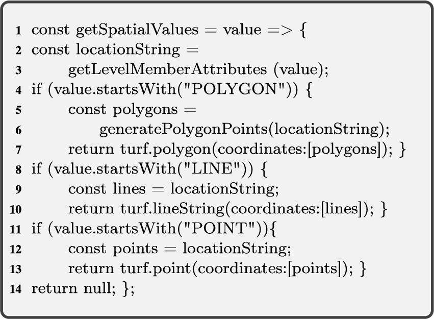
Filtering spatial values Before employing spatial analysis functions, we have to filter the spatial attributes of level members and spatial measures of fact members. Spatial values are always an object (o) value in a triple pattern
We have shown the helper function Algorithm 1 – getSpatialValues, which is used in the main algorithms. We have implemented this helper function on Node.js by filtering the WKT geometries from the input JSON data as exemplified in Listing 6. We create a locationString constant that takes a string value from getLevelMemberAttributes (Line 2). The string value is the last index location of a triple pattern constructed in getLevelMemberAttributes.1919
Finding topological relations Each of the four main enrichment algorithms (Algorithms 3, 4, 5, and 6) returns an instance graph of level members or fact members with topological relations annotated in QB4SOLAP. To find these topological relations we have introduced a helper function in Algorithm 2 – relateSpatialValues. This algorithm is implemented by using boolean functions (spatial predicates) from the Turf.js library for relating spatial values and finding the appropriate topological relations. The library supports the following topological relations with corresponding predicates between certain spatial data types (Table 7). A complete list of functions and details can be found online at http://turfjs.org/docs.
We grouped the available Turf.js spatial boolean functions in Table 7 under three main topological relations (EQUALS, WITHIN, INTERSECTS), with respect to the simplification rules for grouping topological relations (Section 4.1.1) and explained along with Fig. 8 and Table 1. In Table 7, Turf.js built-in functions (predicates) are shown with #boolean prefix. In parentheses, we show how we have named them in our implementation by using the corresponding built-in functions.
Table 7
Turf.js spatial Boolean functions
| EQUALS | WITHIN | INTERSECTS |
| #booleanEqual: (equals) between POINT-POINT LINE-LINE POLYGON-POLYGON | #booleanWithin: (within) between LINE-POLYGON POLYGON-POLYGON #booleanPointInPolygon: (within) between POINT-POLYGON | #booleanCrosses: (crosses) between LINE-POLYGON #booleanOverlap: (overlaps) between POLYGON-POLYGON #booleanPointOnLine: (intersects) between POINT-POLYGON |
Listing 7 provides an overview of the implementation of the boolean functions from Table 7 that are called in the main function for relating spatial values (relateSpatialValues) shown in Listing 8. We provide examples for each of the main topological relations (EQUALS, WITHIN, INTERSECTS).
This first spatial boolean function in Listing 7 is equals (Lines 1–8), which can be between any pair of the same spatial data type (Table 7). We have grouped child level spatial (attribute) values and parent level spatial (attribute) values by their unique id (URI) for each spatial level attribute. This allows us to use javascript array prototype (instance) methods, e.g., every or some, where we can create our own spatial predicate equals with condition to satisfy that every (grouped) child level attribute values should be equal to every (grouped) parent level attribute values. This ensures the multi-point, multi-line, and multi-polygon data types can be covered in our implementation.
For example, in the source data, we had multi-polygons for drainage areas, where each unique drainage areas is a multi-polygon that is composed of several polygons. To simplify we did not store multi-polygon data in RDF. Instead, we have annotated each unique drainage area as several polygons (of the multi-polygon), where each polygon of the drainage area is bound to its drainage area via unique id – URI of the drainage area. This means in the instance graph of parent level members
To handle these multi-polygons, we gather them in a bounding box by using turf.bboxPolygon and turf.bbox functions in Listing 7 (Lines 13–14). In Listing 7 (Lines 10–18) depicts how several polygons of the same parent level can be put into a bounding box, which is passed as a parameter to our second spatial boolean function within. Finally, the function returns in Lines 19–23 with condition to satisfy that every (grouped) child level attribute value should be within the simplified parent level polygon – parentLevelMultipolygonBoundinxBox (Line 23).
Listing 7.
Spatial Boolean functions
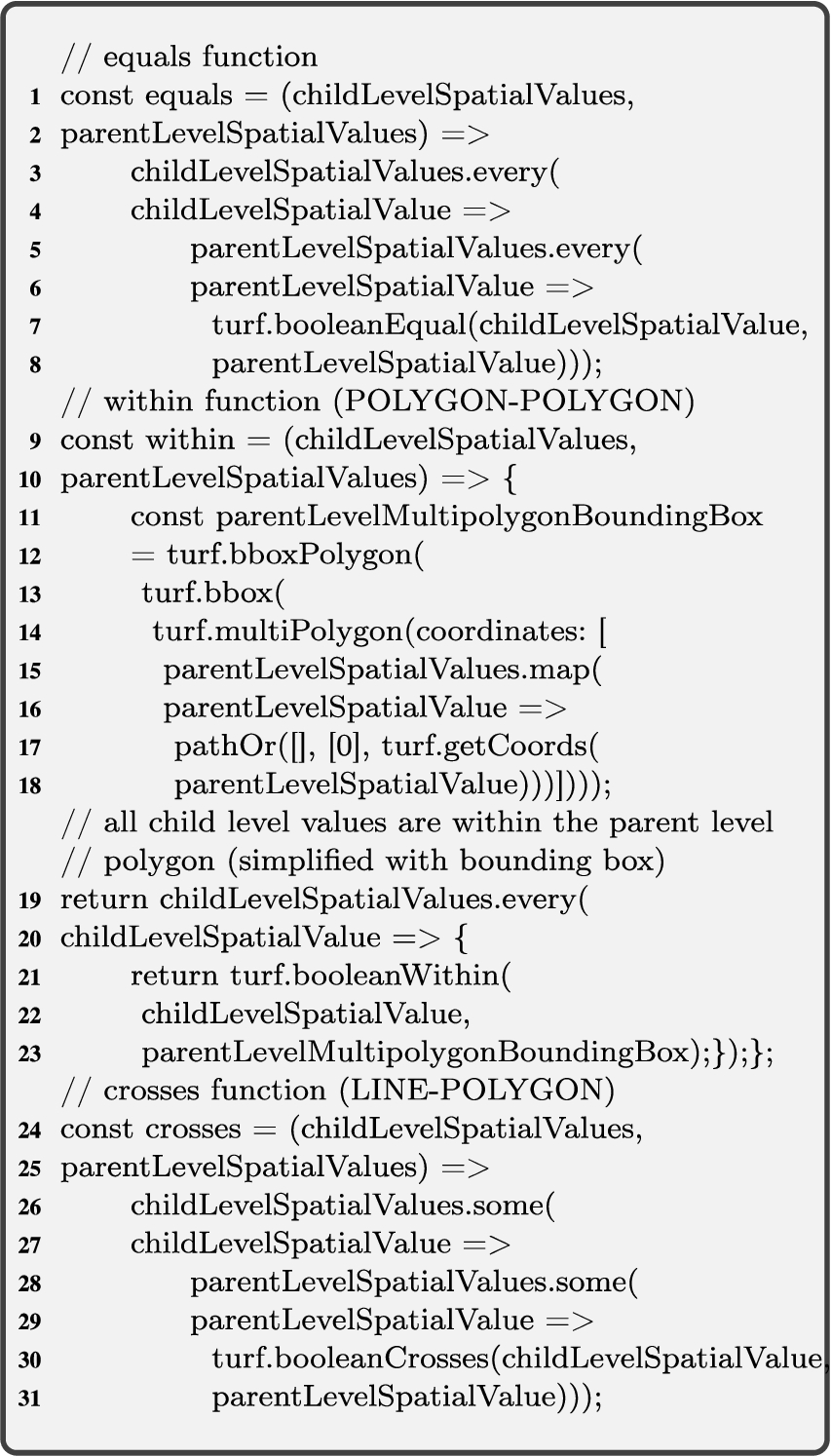
The third spatial boolean function in Listing 7 is crosses (Lines 24–31), where we re-use the Turf.js spatial predicate booleanCrosses. This function is very similar to overlaps in implementation. The only difference is crosses occurs between LINE-POLYGON, overlaps occurs between POLYGON-POLYGON. For both cases, the condition to satisfy is that some of the (grouped) child level attribute values should cross/overlap some of the (grouped) parent level attribute values.
Listing 8.
Relating spatial values
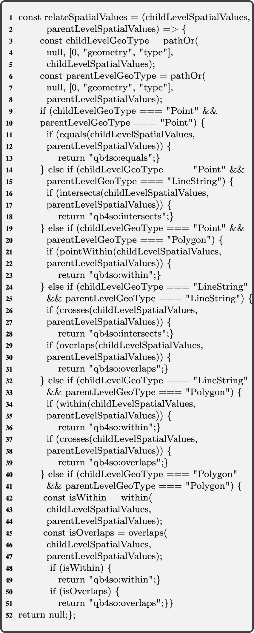
Listing 8 uses our own spatial predicates (explained above) to implement the helper function Algorithm 2 – relateSpatialValues. Note that we have followed the simplification rules for grouping topological relations (Fig. 8), aligned with switch cases for spatial data type pairs from Algorithm 2 in our implementation.
In our implementation illustrated in Listing 8, we create two functions childLevelGeoType (Line 3) and parentLevelGeoType (Line 6), which returns the geometry type of a given attribute value. This way we can implement switch(
Detecting topological relations Finally, we have implemented detecting topological relations algorithms (Algorithms 3 and 5) with a bottom-up approach after implementing the core helper functions. In the following, we show the function implemented on Node.js for detecting topological relations (Listing 9) between level members, which is covered in Algorithm 3. The same approach with minor differences (in parameter passing) is used in our implementation for detecting topological relations between fact-level members (Algorithm 5).
Listing 9.
Detecting topological relations (between level members)
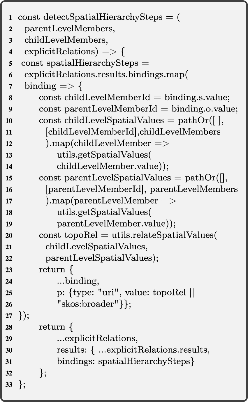
Listing 9 is constructed with the main function detectSpatialHierarchySteps with parameters of parentLevelMembers, childLevelMembers, and explicitRelations.2020 In Line 5, the constant spatialHierachySteps takes the explicitRelations between child level and parent level members, and creates constants for those in Lines 8 and 9. The next step is to get the spatial values of the level members (child level members Lines 10–14 and parent level members Lines 15–19), where we utilize the helper function getSpatialValues, which is described in Listing 6. In Line 20, we create a constant topoRel, which takes the helper function relateSpatialValues (Listing 8) with two parameters childLevelSpatialValues and parentLevelSpatialValues that are created, in Lines 10 and 15, respectively. Next, we return the topological relations (topoRel) as predicates (p) between Lines 24–26. If a topological relation is not found, we keep the explicit relation as skos:broader (Line 26). Finally, we return the new results by replacing the explicitRelations with spatialHierarchySteps (Lines 28–32).
We now discuss our results in Table 3, for both cases covered in Algorithms 3 and 5, together with a number of input level members and fact members.
A.3.Discovering implicit topological relations
Discovering implicit topological relations is addressed in the following algorithms: Algorithm 4 – discoverSpatialHS and Algorithm 6 – discoverFactLevel. In both cases the source data has not any defined roll-up relations (with skos:broader), or has missing spatial hierarchy steps between level members. Similarly, a fact level member has no defined relation link to any spatial level member of its dimensions.
The input variables for Algorithm 4 – discoverSpatialHS are the triples with dimensions (
The input variables for Algorithm 6 – discoverFactLevel are the triples with dimensions (
Listing 10.
Discovering topological relations (schema wrapper)
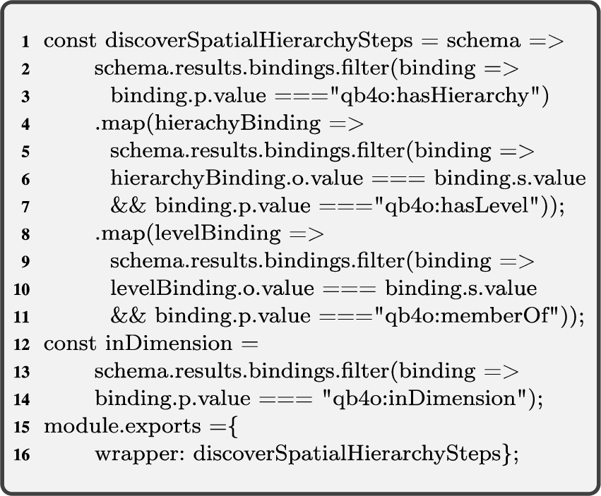
The following listing (Listing 10) shows how we implement a schema wrapper by filtering the schema graph at our endpoint with predicates for schema elements (Lines 3, 7, 11, and 14). Once we get to the levels, we filter the level members in each level with qb4o:memberOf predicate (Line 11). Afterwards, we group level members by level that are in the same hierarchy and pass these grouped level members as inputs to a similar function as in Listing 9, which is called detectSpatialHierarchyStepsExpensive. This function takes only two parameters without explicit relations (two sets of level members grouped by level: parentLevelMembers and childLevelMembers). We run this algorithm several times for each pair of grouped level members (by level) within the same hierarchy as our approach is discovering implicit relations between level members and fact-level members. For fact members we similarly use one parameter (i.e., parentLevelMembers) as the grouped level members (by level), and the other parameter is fact members (i.e., childLevelMembers), which are annotated as qb:Observation. In the detectSpatialHierarchyStepsExpensive function we utilize the same helper functions that are implemented with child-parent topological relations and simplification rules defined in Section 4.1.1 along with Fig. 8 and Table 1. This ensures to apply spatial boolean predicates (on geometries of level members and fact members) with relateSpatialValues helper function only between the appropriate spatial data types given in Tables 1 and 7. Since there are no explicit relations in detectSpatialHierarchyStepsExpensive function, relateSpatialValues helper function is called
We now discuss our results in Table 3 for both cases covered in Algorithms 4 and 6, together with a number of input level members and fact members.
A.4.Generating the fact schema
Finally, we implement the enrichment of the fact schema based on spatially enriched fact instances (members). To extract the input variables for Algorithm 7 – defineSpatialFactDSD, we use the spatially enriched fact members (by Algorithms 5 and 6) and non-spatial fact schema.
The first step of generating the fact schema is to look for detected and discovered topological relations between the fact and level members and then annotate each of them with qb4so:topologicalRelation in the fact schema as given in Listing 3. The next step is to identify the spatial data types with helper functions getMeasures and getSpatialValues (Listings 5 and 6). Finally, for each of the identified spatial data types we annotate the fact schema with the corresponding spatial aggregate function, e.g., spatial data type POINT can have ConvexHull aggregate function, LINE can have Union etc.
In our implementation of detecting and discovering topological relations between fact members and level members, we have only encountered the qb4so:within topological relation. Thus, the fact schema enrichment implementation generates Lines 4 and 5 as exemplified in Listing 3. As spatial measures in fact members, we have found the POINT spatial data type. Therefore, the fact schema enrichment implementation generates Lines 6 and 7, annotating that the spatial measure has qb4so:ConvexHull aggregate function, as exemplified in Listing 3.
After the spatial enrichment is fully completed, both schema2121 and instance2222 data has been published via the same SPARQL endpoint with QB4SOLAP.
References
[1] | A. Abelló, O. Romero, T.B. Pedersen, R. Berlanga, V. Nebot, M.J. Aramburu and A. Simitsis, Using semantic web technologies for exploratory olap: A survey, IEEE Transactions on Knowledge and Data Engineering 27: (2) ((2015) ), 571–588. doi:10.1109/TKDE.2014.2330822. |
[2] | A.B. Andersen, N. Gür, K. Hose, K.A. Jakobsen and T.B. Pedersen, Publishing Danish Agricultural Government data as semantic web data, Semantic Technology 8943: ((2014) ), 178–186. doi:10.1007/978-3-319-15615-6_13. |
[3] | R. Atkinson, QB4ST: RDF data cube extensions for spatio-temporal components, W3C Working Group, (2017) , https://www.w3.org/TR/qb4st/. |
[4] | D. Brickley, Basic geo (WGS84 lat/long) vocabulary, W3C Semantic Web Interest Group, 2003, https://www.w3.org/2003/01/geo/. |
[5] | R.P. Deb Nath, K. Hose and T.B. Pedersen, Towards a programmable semantic extract-transform-load framework for semantic data warehouses, in: Proceedings of the 18th International Workshop on Data Warehousing and OLAP, (2015) , pp. 15–24. doi:10.1145/2811222.2811229. |
[6] | M.J. Egenhofer and J. Herring, A mathematical framework for the definition of topological relationships, in: Fourth International Symposium on Spatial Data Handling, (1990) , pp. 803–813. doi:10.1080/02693799108927841. |
[7] | L. Etcheverry, A. Vaisman and E. Zimányi, Modeling and querying data warehouses on the semantic web using QB4OLAP, in: Data Warehousing and Knowledge Discovery, Vol. 8646: , Springer, (2014) , pp. 45–56. doi:10.1007/978-3-319-10160-6_5. |
[8] | V. Gaede and O. Günther, Multidimensional access methods, ACM Computing Surveys (CSUR) 30: (2) ((1998) ), 170–231. doi:10.1145/280277.280279. |
[9] | L. Galárraga, K. Ahlstrøm, K. Hose and T.B. Pedersen, Answering provenance-aware queries on RDF data cubes under memory budgets, in: The Semantic Web – ISWC 2018, Springer International Publishing, Cham, (2018) , pp. 547–565. doi:10.1007/978-3-030-00671-6_32. |
[10] | L. Galárraga, K.A.M. Mathiassen and K. Hose, QBOAirbase: The European air quality database as an rdf cube, in: International Semantic Web Conference (Posters, Demos & Industry Tracks), (2017) . |
[11] | E. Gallinucci, M. Golfarelli, S. Rizzi, A. Abelló and O. Romero, Interactive multidimensional modeling of linked data for exploratory olap, Information Systems ((2018) ). doi:10.1016/j.is.2018.06.004. |
[12] | N. Gür, K. Hose, T.B. Pedersen and E. Zimányi, Enabling spatial OLAP over environmental and farming data with QB4SOLAP, in: Semantic Technology, Vol. 10055: , Springer, (2016) , pp. 287–304. doi:10.1007/978-3-319-50112-3_22. |
[13] | N. Gür, K. Hose, E. Zimányi and T.B. Pedersen, Modeling and querying spatial data warehouses on the semantic web, in: Semantic Technology, Vol. 9544: , Springer, (2015) , pp. 1–20. doi:10.1007/978-3-319-31676-5_1. |
[14] | N. Gür, J. Nielsen, K. Hose and T.B. Pedersen, GeoSemOLAP: SOLAP on the semantic web made easy, in: Proceedings of the 26th International Conference on World Wide Web, (2017) , pp. 213–217. doi:10.1145/3041021.3054731. |
[15] | N. Gür, T.B. Pedersen, E. Zimányi and K. Hose, A foundation for spatial data warehouses on the semantic web, Semantic Web Journal 9: (5) ((2018) ), 557–587. doi:10.3233/SW-170281. |
[16] | A. Harth, K. Hose and R. Schenkel (eds), Linked Data Management, Chapman and Hall/CRC, (2014) . doi:10.1201/b16859. |
[17] | O. Hartig, K. Hose and J.F. Sequeda, Linked data management, in: Encyclopedia of Big Data Technologies, S. Sakr and A.Y. Zomaya, eds, Springer, (2019) . doi:10.1007/978-3-319-63962-8_76-1. |
[18] | K. Hose and R. Schenkel, RDF stores, in: Encyclopedia of Database Systems, L. Liu and M.T. Özsu, eds, 2nd edn, Springer, (2018) . doi:10.1007/978-1-4614-8265-9_80676. |
[19] | W. Huang, S.A. Raza, O. Mirzov and L. Harrie, Assessment and benchmarking of spatially enabled RDF stores for the next generation of spatial data infrastructure, ISPRS International Journal of Geo-Information 8: (7) ((2019) ), 310. doi:10.3390/ijgi8070310. |
[20] | B. Hyland and B.V. Terrazas, Cookbook for open government linked data, W3C Government Linked Data Working Group, (2011) , https://www.w3.org/2011/gld/wiki/Linked_Data_Cookbook. |
[21] | D. Ibragimov, K. Hose, T.B. Pedersen and E. Zimányi, Processing aggregate queries in a federation of SPARQL endpoints, in: The Semantic Web. Latest Advances and New Domains – 12th European Semantic Web Conference, ESWC 2015, Portoroz, Slovenia, May 31–June 4, 2015. Proceedings, (2015) , pp. 269–285. doi:10.1007/978-3-319-18818-8_17. |
[22] | D. Ibragimov, K. Hose, T.B. Pedersen and E. Zimányi, Towards exploratory OLAP over linked open data – a case study, in: Enabling Real-Time Business Intelligence, Springer, (2015) , pp. 114–132. doi:10.1007/978-3-662-46839-5_8. |
[23] | D. Ibragimov, K. Hose, T.B. Pedersen and E. Zimányi, Optimizing aggregate SPARQL queries using materialized RDF views, in: The Semantic Web: 15th International Semantic Web Conference (ISWC’16), Springer, (2016) , pp. 341–359. doi:10.1007/978-3-319-46523-4_21. |
[24] | T. Ioannidis, G. Garbis, K. Kyzirakos, K. Bereta and M. Koubarakis, Evaluating geospatial RDF stores using the benchmark Geographica 2, 2019, arXiv preprint, https://arxiv.org/abs/1906.01933 arXiv:1906.01933. |
[25] | K.A. Jakobsen, A.B. Andersen, K. Hose and T.B. Pedersen, Optimizing RDF data cubes for efficient processing of analytical queries, in: COLD, (2015) , http://ceur-ws.org/Vol-1426/paper-02.pdf. |
[26] | B. Kämpgen and A. Harth, No size fits all – running the star schema benchmark with SPARQL and RDF aggregate views, in: Extended Semantic Web Conference, Springer, (2013) , pp. 290–304. doi:10.1007/978-3-642-38288-8_20. |
[27] | B. Kämpgen, S. O’Riain and A. Harth, Interacting with statistical linked data via OLAP operations, in: The Semantic Web: ESWC 2012 Satellite Events, Vol. 7540: , Springer, (2012) , pp. 87–101. doi:10.1007/978-3-662-46641-4_7. |
[28] | K. Kyzirakos, D. Savva, I. Vlachopoulos, A. Vasileiou, N. Karalis, M. Koubarakis and S. Manegold, GeoTriples: Transforming geospatial data into RDF graphs using R2RML and RML mappings, Journal of Web Semantics 52: ((2018) ), 16–32. doi:10.1016/j.websem.2018.08.003. |
[29] | E. Malinowski and E. Zimányi, Representing spatiality in a conceptual multidimensional model, in: Proceedings of the 12th Annual ACM International Workshop on Geographic Information Systems, GIS’04, ACM, New York, NY, USA, (2004) , pp. 12–22, http://doi.acm.org/10.1145/1032222.1032226. doi:10.1145/1032222.1032226. |
[30] | A. Miles and S. Bechhofer, SKOS Simple Knowledge Organization System namespace document, W3C Recommendation, 2009, https://www.w3.org/TR/skos-reference/. |
[31] | R.P.D. Nath, K. Hose, T.B. Pedersen and O. Romero, SETL: A programmable semantic extract-transform-load framework for semantic data warehouses, Information Systems 68: ((2017) ), 17–43. doi:10.1016/j.is.2017.01.005. |
[32] | R.P.D. Nath, K. Hose, T.B. Pedersen, O. Romero and A. Bhattacharjee, SETLBI: an integrated platform for semantic business intelligence, in: Companion of the 2020 Web Conference 2020, Taipei, Taiwan, April 20–24, 2020, (2020) , pp. 167–171. doi:10.1145/3366424.3383533. |
[33] | S. Neumaier and A. Polleres, Geo-semantic labelling of open data, SEMANTiCS 2018 – 14th International Conference on Semantic Systems, Procedia Computer Science ((2018) ). doi:10.1016/j.procs.2018.09.002. |
[34] | Open Geospatial Consortium, GeoSPARQL: A geographic query language for RDF data, W3C Recommendation, 2014. |
[35] | K. Patroumpas, N. Georgomanolis, T. Stratiotis, M. Alexakis and S. Athanasiou, Exposing INSPIRE on the semantic web, Web Semantics 35: (P1) ((2015) ), 53–62. doi:10.1016/j.websem.2015.09.003. |
[36] | D. Pedersen, J. Pedersen and T.B. Pedersen, Integrating XML data in the TARGIT OLAP system, in: Proceedings. 20th International Conference on Data Engineering, IEEE, (2004) , pp. 778–781. doi:10.1109/ICDE.2004.1320045. |
[37] | D. Pedersen, K. Riis and T.B. Pedersen, Query optimization for OLAP-XML federations, in: Proceedings of the 5th International Workshop on Data Warehousing and OLAP (DOLAP’02), ACM, (2002) , pp. 57–64. doi:10.1145/583890.583899. |
[38] | S. Rivest, Y. Bédard, M.-J. Proulx, M. Nadeau, F. Hubert and J. Pastor, SOLAP technology: Merging business intelligence with geospatial technology for interactive spatio-temporal exploration and analysis of data, ISPRS Journal of Photogrammetry and Remote Sensing 60: (1) ((2005) ), 17–33. doi:10.1016/j.isprsjprs.2005.10.002. |
[39] | G. Rojas, G. Giannopoulos and J.J.L. Daniel Hladky, Managing geospatial linked data in the GeoKnow project, in: The Semantic Web in Earth and Space Science. Current Status and Future Directions, Vol. 20: , IOS Press, (2015) , p. 51. doi:10.3233/978-1-61499-501-2-51. |
[40] | J.M. Salas and A. Harth, NeoGeo vocabulary specification, GeoVocab Working Group, (2012) , http://geovocab.org/doc/neogeo/. |
[41] | C. Stadler, J. Lehmann, K. Höffner and S.A. Linkedgeodata, A core for a web of spatial open data, Semantic Web 3: (4) ((2012) ), 333–354, https://dl.acm.org/doi/10.5555/2590208.2590210. doi:10.3233/SW-2011-0052. |
[42] | A. Vaisman and E. Zimányi, Spatial data warehouses, in: Data Warehouse Systems, Springer, (2014) , pp. 427–473. doi:10.1007/978-3-642-54655-6. |
[43] | J. Varga, L. Etcheverry, A.A. Vaisman, O. Romero, T.B. Pedersen and C. Thomsen, QB2OLAP: enabling OLAP on statistical linked open data, in: 32nd IEEE International Conference on Data Engineering, (2016) , pp. 1346–1349. doi:10.1109/ICDE.2016.7498341. |
[44] | J. Varga, A.A. Vaisman, O. Romero, L. Etcheverry, T.B. Pedersen and C. Thomsen, Dimensional enrichment of statistical linked open data, in: Web Semantics: Science, Services and Agents on the World Wide Web, Vol. 40: , Elsevier, (2016) , pp. 22–51. doi:10.1016/j.websem.2016.07.003. |
[45] | M. Wick and B. Vatant, Geo names ontology, GeoNames, (2012) , http://www.geonames.org/ontology. |
[46] | World Wide Web Consortium, SPARQL query language for RDF, W3C Recommendation, 2008, https://www.w3.org/TR/sparql11-query/. |
[47] | World Wide Web Consortium, Data cube implementations, 2011, https://www.w3.org/2011/gld/wiki/Data_Cube_Implementations. |
[48] | World Wide Web Consortium, The RDF data cube vocabulary, W3C Recommendation, 2014, https://www.w3.org/TR/vocab-data-cube/. |
[49] | X. Yin and T.B. Pedersen, Evaluating XML-extended OLAP queries based on physical algebra, Journal of Database Management (JDM) 17: (2) ((2006) ), 85–116. doi:10.4018/jdm.2006040105. |
[50] | E. Zimanyi, Advanced Data Warehouse Design: From Conventional to Spatial and Temporal Applications. Data-Centric Systems and Applications, Springer, (2008) . doi:10.1007/978-3-540-74405-4. |

