
The Dual-Dagum family of distributions: Properties, regression and applications to COVID-19 data
Abstract
A new Dual-Dagum-G (DDa-G) family is defined as a good competitor to the Beta-G and Kumaraswamy-G generators, which are widely applied in several areas. Some of its mathematical properties are addressed. We obtain the maximum likelihood estimates, and some simulations prove the consistency of the estimates. The flexibility of this family is shown through a COVID-19 data set. We propose a new regression based on a special distribution of the DDa-G family, and provide a sensitivity analysis by using data from 1,951 COVID-19 patients collected in Curitiba, Brazil.
1.Introduction
Over the last few decades, many generators have been studied in the distribution theory literature. Two generators that stand out are the Beta-G (B-G) (Eugene et al., 2002) and Kumaraswamy-G (Kw-G) (Cordeiro & de Castro, 2011) classes.
Regarding the B-G family, we can say that, although it contains the incomplete and complete beta functions, its flexibility in terms of adjustment to real data is widespread. Several authors introduced new distributions in this family in different contexts: cancer recurrence (Paranaíba et al., 2011), waiting times before service of 100 bank customers (Abd El-Bar & Ragab, 2015), test on the endurance of deep groove ball bearings (Abu-Zinadah & Bakoban, 2017), survival times of 33 patients suffering from acute Myelogeneous Leukaemia (Mead et al., 2017), among others. More than one-hundred different published distributions in this class can be found to date.
The second family stands out because of the simplicity of its density function, which does not include complicated functions. Further, its suitability for the most diverse types of data sets is widely discussed in the literature. We can cite, for example, the work that originated this family and used data from adult numbers of T. confusum cultured at 29
We know through an analysis of these works that the fits of both classes to real data have a better performance compared to other known classes. We can note that the data sets studied in the aforementioned works are of different types. However, many authors end up repeating the same data sets used in previous works by other authors.
In this sense, we define a new class from the Dagum distribution (Dagum, 1975) and use data bases never published before. The data bases in question concern a very current topic: COVID-19. We understand the importance of studies on this pandemic that impacted the world, and then use COVID-19 data from two cities in Brazil.
The remainder of the paper is organized as follows. Section 2 defines the new family. In Section 3, we present some of its generated distributions. The main properties of the new family are reported in Section 4. Estimation including the case of censoring is addressed in Section 5. A simulation study is done in Section 6. In Section 7, we construct the Log-Dual-Dagum-Weibull regression, and estimate the parameters. Two applications to real data are reported in Section 8, including a regression application and a sensitivity analysis. Conclusions end the paper in Section 9.
2.The new family
The new generator is defined based on the survival function of the Dagum distribution (Dagum, 1977). Kleiber and Kotz (2003) and Kleiber (2008) analyzed characteristics and properties of this distribution. The Dagum distribution presents forms of the increasing, decreasing, bathtub and inverted bathtub risk function (Domma, 2002). This behavior has aroused the interest of several authors to study it in survival analysis (Domma et al., 2011a, b). In this sense, we propose the Dual-Dagum-G (DDa-G) family.
Let
(1)
where
Henceforth, Eq. (1) refers to the random variable
The probability density function (pdf) of
(2)
where
Equations (1) and (2) do not involve complicated mathematical functions, which is an advantage of this family when compared, for example, with the Beta generator.
The hazard rate function (hrf) of
3.Special DDa-G distributions
3.1Dual-Dagum-Weibull (DDa-W)
The DDa-W density (for
(3)
where all parameters are positive. For
3.2Dual-Dagum-log-logistic (DDa-LL)
The cdf of the log-logistic (LL) distribution is (for
Inserting this expression and its derivative in Eq. (2) leads to the DDa-LL density (for
Figure 1.
Shapes of the (a)
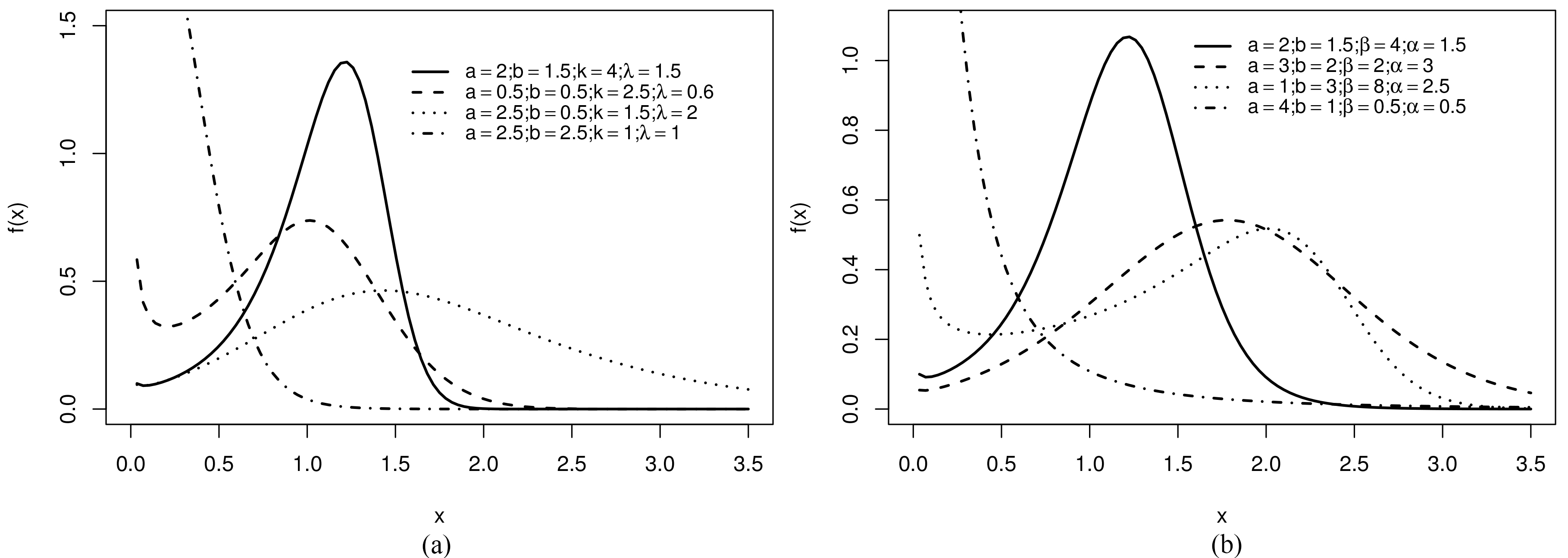
Figure 2.
Shapes of the (a)
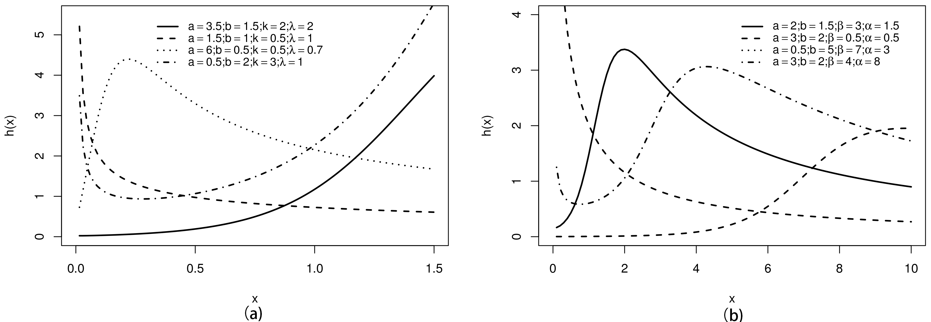
Figures 1 and 2 display shapes of the pdf and hrf of the previous generated models, which show their flexibility in fitting data with different shapes. For example, the Weibull pdf presents only decreasing and unimodal shapes, whereas the DDaW pdf has an extra shape: decreasing-increasing-decreasing.
4.Some properties
4.1Linear representation
For any real
(4)
where
and
By using Eq. (4) in Eq. (1) gives
By expanding the binomial term,
where
where
Next, we use a theorem of Henrici (1993) for a power series raised to any real power different from zero
(5)
where the coefficients are determined recursively from
Formulas for other functions may be found in Hairer et al. (1993).
A random variable
Table 1
Simulation results for the MLEs
| Setup | Sample size | Parameter | Average | Bias | MSE |
|---|---|---|---|---|---|
| Setup 1 |
| 6.08333 | 0.08333 | 0.57738 | |
|
| 0.50948 | 0.00948 | 0.00564 | ||
|
| 0.70188 | 0.00188 | 0.00185 | ||
|
| 6.03727 | 0.03727 | 0.26878 | ||
|
| 0.50437 | 0.00437 | 0.00268 | ||
|
| 0.70065 | 0.00065 | 0.00094 | ||
|
| 6.03482 | 0.03482 | 0.17810 | ||
|
| 0.50325 | 0.00325 | 0.00173 | ||
|
| 0.70019 | 0.00019 | 0.00062 | ||
| Setup 2 |
| 5.57856 | 0.07856 | 0.47019 | |
|
| 0.76402 | 0.01402 | 0.01268 | ||
|
| 0.60096 | 0.00096 | 0.00126 | ||
|
| 5.53366 | 0.03366 | 0.21645 | ||
|
| 0.75664 | 0.00664 | 0.00602 | ||
|
| 0.60048 | 0.00048 | 0.00063 | ||
|
| 5.53103 | 0.03103 | 0.14320 | ||
|
| 0.75506 | 0.00505 | 0.00387 | ||
|
| 0.60006 | 0.00006 | 0.00042 | ||
| Setup 3 |
| 6.59325 | 0.09325 | 0.65217 | |
|
| 0.81513 | 0.01513 | 0.01443 | ||
|
| 0.75093 | 0.00093 | 0.00139 | ||
|
| 6.53986 | 0.03986 | 0.30061 | ||
|
| 0.80719 | 0.00719 | 0.00684 | ||
|
| 0.75030 | 0.00030 | 0.00069 | ||
|
| 6.53657 | 0.03657 | 0.19869 | ||
|
| 0.80534 | 0.00534 | 0.00441 | ||
|
| 0.75002 | 0.00002 | 0.00046 |
By differentiating Eq. (5) and using the concept of exp-G distribution, we can write
(6)
where
Equation (6) is the linear representation for the DDa-G family density in terms of exp-G densities. So, it can provide some mathematical properties for sub-models of the new family from exp-G properties.
4.2Quantile function
Let
(7)
Equation (7) reveals that the qf of the proposed family is a function of the baseline qf.
The skewness and kurtosis of
and
reported by Kenney and Keeping (1961) and Moors (1988), respectively.
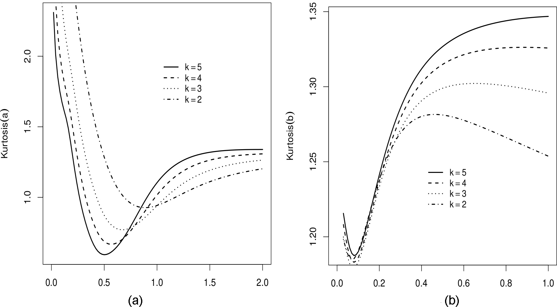
Figures 3 and 4 display the skewness and kurtosis of the DDa-W distribution as functions of both
Figure 3.
Bowley’s skewness of the DDa-W distribution. (a) as function of
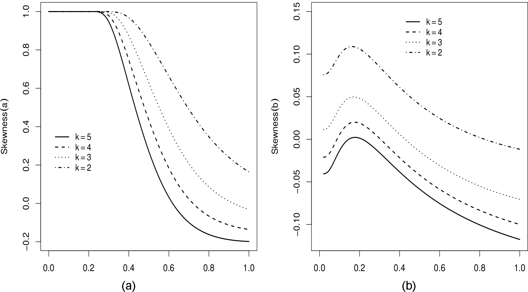
Figure 4.
Moors’ kurtosis of the DDa-W distribution. (a) as function of
4.3Moments
From now on, let
Moments for several exp-G distributions reported by Nadarajah and Kotz (2006) give
4.4Generating functions
The generating function (gf)
where
5.Estimation
The estimation of the unknown parameters of the DDa-G distribution is performed by the maximum likelihood method. Let
The R software has the AdequacyModel computational library (Marinho et al., 2019) as a good alternative for maximizing
6.Simulation study
We adopt the exponential (E) baseline (with the expected value
1. Generate
2. Return
We consider 2,000 Monte Carlo replications and the BFGS algorithm in the R software for maximizing the log-likelihood, obtain the MLEs and their averages, biases and mean square errors (MSEs). The simulation process is carried out as below:
1. Simulate DDa-E observations for fixed
2. Three scenarios considered are:
3. We calculate the MLEs from each generated data set, and obtain the averages, biases and MSEs.
Table 1 reports these findings. The average estimates converge to the true parameter values and the biases decrease when
7.Log-Dual-Dagum-Weibull (LDDa-W) regression
If
(8)
where
The survival function corresponding to Eq. (8) is
The pdf of the standardized random variable
(9)
The lifetimes
The LDDa-W regression for the response variable
(10)
where
Let
(11)
where
8.Applications
The Weibull and Birnbaum-Saunders distributions are taken as baselines to prove the flexibility of the new family. The data sets were obtained from the open data portal of the Federal Government linked to the Ministry of Health and comprise events from 2020–2021 (accessed on August 23, 2021). The data portal is available at https://dados.gov.br/dataset/bd-srag-2020.
All computations are done in R using
GenSA,
MASSand
AdequacyModellibraries, and the
goodness.fit()function with the “
SANN” method. The initial parameter values to maximize the log-likelihood were obtained through a heuristic method by using the
MASSpackage in the R language.
The new distributions are compared with well-known models belonging to the Kw-G and B-G classes using the statistics: Cramér-von Mises (
• The Kumaraswamy-Weibull (Kw-W) density (Cordeiro et al., 2010) (for
• The Beta Weibull (B-W) density (Lee et al., 2007), and explored by Cordeiro et al. (2013) (for
where
• The Beta-Birnbaum-Saunders (B-BS) density (Cordeiro & Lemonte, 2011) (for
• The Kumaraswamy-Birnbaum-Saunders (Kw-BS) density (Saulo et al., 2012) (for
In the following, we calculate descriptive statistics, MLEs, their standard errors (SEs) and adequacy statistics to compare the fitted distributions to the data sets.
8.1COVID-19 data in Recife
The first application represents the times (in days) of 564 COVID-19 patients from the date of entry in the Intensive Care Unit (ICU) until cure in Recife (State of Pernambuco). In this context, the cure characterizes the evolution of the case as hospital discharge. Discharge from hospital can only mean that the patient no longer needs hospitalization.
The descriptive statistics for the time until cure for COVID-19 data in Recife include: mean
The values of the statistics
Table 2
Parameter estimation results for COVID-19 times in Recife, and adequacy measures
| Distribution | MLEs and SEs |
|
|
| ||||
|---|---|---|---|---|---|---|---|---|
| DDa-W |
|
|
|
| 0.14252 | 0.98512 | 0.04054 | 0.3121 |
| 6.72231 | 0.39752 | 0.52249 | 37.76017 | |||||
| (0.01294) | (0.01831) | (0.01294) | ( | |||||
| DDa-BS |
|
|
|
| 0.21022 | 1.38258 | 0.04364 | 0.2331 |
| 3.30213 | 0.42399 | 1.33094 | 13.4665 | |||||
| (0.40970) | (0.03065) | (0.12385) | (2.967e-06) | |||||
| Kw-W |
|
|
|
| 0.37456 | 2.23561 | 0.05660 | 0.05389 |
| 19.77064 | 1.84816 | 0.32830 | 0.59472 | |||||
| (2.27358) | (0.77297) | (0.04448) | (0.16338) | |||||
| Kw-BS |
|
|
|
| 0.56382 | 3.35188 | 0.06824 | 0.01047 |
| 4.67480 | 40.85901 | 5.42802 | 89.55090 | |||||
| (0.16191) | (3.29676) | (0.12325) | (0.01177) | |||||
| BW |
|
|
|
| 0.42545 | 2.48047 | 0.06282 | 0.02334 |
| 77.06372 | 47.75535 | 0.13930 | 19.46675 | |||||
| (4.713e-03) | (1.404e-04) | (4.095e-03) | (0.02961) | |||||
| Beta-BS |
|
|
|
| 0.78468 | 4.42605 | 0.07809 | 0.00205 |
| 6.41931 | 10.69270 | 37.27032 | 34.29943 | |||||
| (0.19522) | (0.40651) | (0.04304) | (0.03022) | |||||
| Weibull |
|
| 1.8997 | 10.20654 | 0.11559 | 5.702e-07 | ||
| 1.18881 | 22.24782 | |||||||
| (0.03583) | (0.83527) | |||||||
| BS |
|
| 0.69621 | 4.13159 | 0.07788 | 0.00214 | ||
| 0.94854 | 14.34992 | |||||||
| (0.02826) | (0.51174) | |||||||
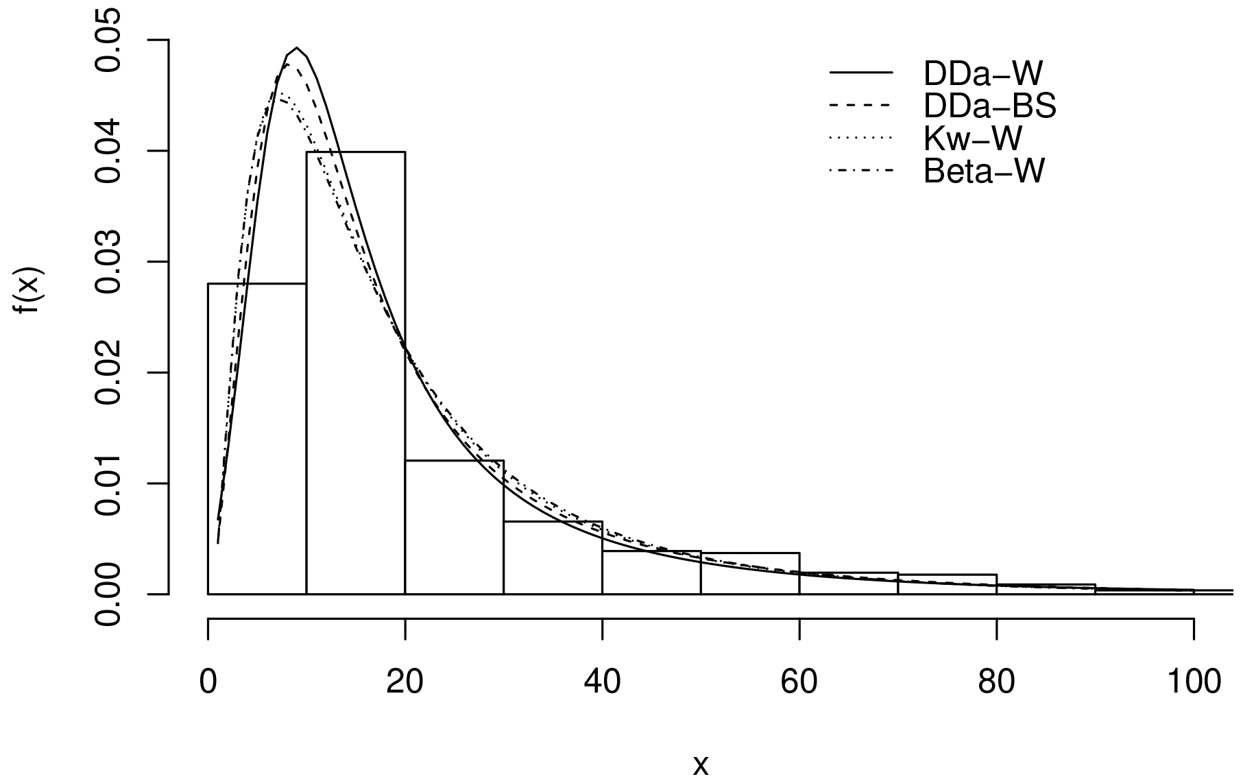
The Vuong test (Vuong, 1989) also reveals that the DDa-W distribution is better than the DDa-BS (
Figure 5 displays the histogram of the data, where
8.2Regression modeling applied to COVID-19 data in Curitiba (Brazil)
The study comprises the time (in days) elapsed from the date of hospitalization until death by the coronavirus, of 1,951 patients in Curitiba-PR, with all observations failing, that is, censored times were not considered in the study, with occurrences of death in 2020 and 2021.
The explanatory variables are (for
•
•
The computational part is developed in R using
survivallibrary, with
optim()function, and the “
SANN” method.
We adopt the Akaike information criterion (AIC), corrected Akaike information criterion (CAIC), and Bayesian information criterion (BIC) to choose the appropriate model. We compare the fits of the LDDa-W Eq. (8) with the log-Kumaraswamy-Weibull or Kumaraswamy Gumbel (Kw-Gu) (Cordeiro et al., 2012), log-beta Weibull (LBW) and log-Weibull (LW) models. The densities for the alternative regressions are reported below:
Table 3
Estimation results from some fitted regressions to the COVID-19 data in Curitiba, and the adequacy measures
| LDDa-W | Kw-Gu | LBW | LW | |||||
|---|---|---|---|---|---|---|---|---|
| Parameter | Estimate | SE | Estimate | SE | Estimate | SE | Estimate | SE |
|
| 5.635 | 0.419 | 3.496 | 0.311 | 3.378 | 0.508 | 4.090 | 0.100 |
|
| 0.035 | 0.037 | 0.039 | 0.035 | ||||
|
| 0.001 | 0.001 | 0.001 | 0.001 | ||||
|
| 2.355 | 0.349 | 1.419 | 0.186 | 1.973 | 0.608 | 0.758 | 0.012 |
|
| 5.876 | 0.709 | 3.076 | 0.795 | 6.065 | 3.688 | – | – |
|
| 1.677 | 0.348 | 1.813 | 0.234 | 3.492 | 1.124 | – | – |
| AIC | 4880.25 | 4882.50 | 4895.15 | 4990.87 | ||||
| CAIC | 4880.29 | 4882.54 | 4895.19 | 4990.89 | ||||
| BIC | 4913.70 | 4915.95 | 4928.61 | 5013.18 | ||||
Figure 5.
Estimated DDa-W, DDa-BS, Kw-W and Beta-W densities.
• The LW (or Gumbel) density function
where
• The LBW density function
where
• The Kw-Gu density function
where
The failure rate function is useful to aid in model identification more suitable for the variable time. In this context, the TTT plot (not shown here) for the data under study shows an increasing appearance for the most part, but due to its final behavior, it indicates an inverting bathtub risk function. The descriptive statistics for the time until death for COVID-19 data in Curitiba include: mean
Next, we provide results from the fit of the regression
(12)
where
Table 3 provides some findings from the regressions fitted to the current data. They indicate that LDDa-W model provides the best fit to the data. Further, all covariates (
Thus, the time to death decreases when the age increases. Regarding the patient’s gender, male patients present smaller time until death than female patients, since the estimate of its coefficient is negative.
After the LDDa-W regression estimation, the plots of the empirical and estimated survival functions support the model adequacy to these data.
Also, as part of the analysis, it is important to verify if there are observations influencing the model’s adjustment. A sensitivity analysis was carried out to investigate this fact using the Cook’s distance and will be presented below.
8.2.1Sensitivity analysis and influential observations
Under the Generalized Cook Distance (Cook, 1977), the observations #349, #826 and #897 are the ones that stand out the most, thus indicating that they can be possible influential observations.
The observation #349 refers to a female individual, aged 84 years and with a time of hospitalization until death of 172 days. The observation #826 is identified as a 78-year-old male and has a time to death of 6 days. And the observation #897 refers to the male individual aged 61 years old, whose hospitalization time until death was only 3 days. The observations #349, #826 and #897 represent individuals with peculiar behaviors, but do not show signs of error in data collection or transcription, and therefore must be kept in the database. The final model is given in Eq. (12).
The impact of possible influential observations detected should be analyzed in order to assess the estimates and sensitivity of the model. This analysis considers new estimates for the model parameters from sub-samples referring to the withdrawal of these observations individually and in groups.
It is considered that the changes in the estimated values for the parameters are not very expressive and there is significance of the explanatory variables when considering the level of 10%. In addition, there was no change in the sign of the coefficient of the explanatory variables, so the inclusion or exclusion of the identified observations does not presuppose changes in the interpretation of the results.
9.Conclusions
One of the main objectives of distribution theory is to define a family of models to better explain lifetime phenomenon in several areas of knowledge. We proposed the Dual-Dagum-G (“DDa-G”) family, which can generalize all classical continuous distributions. Its parameters are estimated by maximum likelihood, and a simulation study showed the consistency of the estimators. We showed the flexibility of the new family by means of two real COVID-19 data sets. We proved that the new Log-Dual-Dagum-Weibull (LDDaW) regression outperformed regressions based on well-known Kumaraswamy-G and Beta-G generators. After verifying the good fit of the new regression, a sensitivity analysis was performed, where it was possible to verify the occurrence of influential observations. As future work, it could be interesting to investigate other methods of sensitivity analysis, such as the local influence, if the results obtained through the Cook Distance prevail and still carry out a residual analysis for the new regression model.
Note: Computer codes in
Rlanguage can be provided to readers free upon request.
References
[1] | Aarset, M.V. ((1987) ). How to identify a bathtub hazard rate. IEEE Transactions on Reliability, 36: , 106-108. |
[2] | Abd El-Bar, A.M.T., & Ragab, I.E. ((2015) ). The beta generalized inverted exponential distribution. International Information Institute, 18: , 421-430. |
[3] | Abu-Zinadah, H.H., & Bakoban, R.A. ((2017) ). The Beta Generalized Inverted Exponential Distribution with real data applications. Revstat – Statistical Journal, 15: , 65-88. |
[4] | Cook, R.D. ((1977) ). Detection of influential observation in linear regression. Technometrics, 19: , 15-18. |
[5] | Cordeiro, G.M., & de Castro, M. ((2011) ). A new family of generalized distributions. Journal of Statistical Computation and Simulation, 81: , 883-898. |
[6] | Cordeiro, G.M., & Lemonte, A.J. ((2011) ). The β-Birnbaum-Saunders distribution: An improved distribution for fatigue life modeling. Computational Statistics & Data Analysis, 55: , 1445-1461. |
[7] | Cordeiro, G.M., Nadarajah, S., & Ortega, E.M.M. ((2012) ). The kumaraswamy gumbel distribution. Statistical Methods & Applications, 21: , 139-168. |
[8] | Cordeiro, G.M., Nadarajah, S., & Ortega, E.M.M. ((2013) ). General results for the beta Weibull distribution. Journal of Statistical Computation and Simulation, 83: , 1082-1114. |
[9] | Cordeiro, G.M., Ortega, E.M.M., & Nadarajah, S. ((2010) ). The Kumaraswamy Weibull distribution with application to failure data. Journal of the Franklin Institute, 347: , 1399-1429. |
[10] | Cordeiro, G.M., Saboor, A., Khan, M.N., Ozel, G., & Pascoa, M.A.R. ((2016) ). The kumaraswamy exponential-weibull distribution: Theory and applications. Hacettepe Journal of Mathematics and Statistics, 45: , 1203-1229. |
[11] | Dagum, C. ((1975) ). A model of income distribution and the conditions of existence of moments of finite order. Bulletin of the International Statistical Institute, 46: , 199-205. |
[12] | Dagum, C. ((1977) ). A new model of personal income-distribution-specification and estimation. Economie Appliquáe, 30: , 413-437. |
[13] | Domma, F. ((2002) ). L’andamento della hazard function nel modello di Dagum a tre parametri. Quaderni di Statistica, 4: , 1-12. |
[14] | Domma, F., Giordano, S., & Zenga, M. ((2011) a). Maximum likelihood estimation in Dagum distribution with censored samples. Journal of Applied Statistics, 38: , 2971-2985. |
[15] | Domma, F., Latorre, G., & Zenga, M. ((2011) b). Reliablity studies of Dagum distribution. Working Paper, 206: , 1-17. |
[16] | Eugene, N., Lee, C., & Famoye, F. (2002) Beta-normal distribution and its applications. Communications in Statistics – Theory and Methods, 31: , 497-512. |
[17] | Hairer, E., Norsett, S., & Wanner, G. ((1993) ). Solving Ordinary Differential Equations I. Springer, 8: , 528. |
[18] | Henrici, P. ((1993) ). Applied and Computational Complex Analysis, Volume 3: Discrete Fourier analysis-Cauchy integrals-Construction of Conformal Maps-Univalent Functions. John Wiley & Sons Inc., 3: , 656. |
[19] | Johnson, N.L., Kotz, S., & Balakrishnan, N. ((1995) ). Continuous univariate distributions. John Wiley & Sons, 2: , 732. |
[20] | Kenney, J.F., & Keeping, E.S. ((1961) ). Mathematics of statistics. D. Van Nostrand Company, 1: , 429. |
[21] | Kleiber, C. ((2008) ). A guide to the Dagum distributions. Modeling Income Distributions and Lorenz Curves – Springer, 5: , 97-117. |
[22] | Kleiber, C., & Kotz, S. ((2003) ). Statistical size distributions in economics and actuarial sciences. John Wiley & Sons, 470: , 352. |
[23] | Lee, C., Famoye, F., & Olumolade, O. ((2007) ). Beta-weibull distribution: Some properties and applications to censored data. Journal of Modern Applied Statistical Methods, 6: , 173-186. |
[24] | Mameli, V. ((2015) ). The Kumaraswamy skew-normal distribution. Statistics & Probability Letters, 104: , 75-81. |
[25] | Marinho, P.R.D., Silva, R.B., Bourguignon, M., Cordeiro, G.M., & Nadarajah, S. ((2019) ). AdequacyModel: An R package for probability distributions and general purpose optimization. PLoS ONE, 14: , e0221487. |
[26] | Mead, M., Afify, A.Z., Hamedani, G., & Ghosh, I. ((2017) ). The beta exponential fréchet distribution with applications. Austrian Journal of Statistics, 46: , 41-63. |
[27] | Moors, J. ((1988) ). A quantile alternative for kurtosis. Journal of the Royal Statistical Society. Series D (The Statistician), 37: , 25-32. |
[28] | Nadarajah, S., & Kotz, S. ((2006) ). The exponentiated type distributions. Acta Applicandae Mathematica, 92: , 97-111. |
[29] | Ortega, E.M., Cordeiro, G.M., & Kattan, M.W. ((2013) ). The log-beta weibull regression model with application to predict recurrence of prostate cancer. Statistical Papers, 54: , 113-132. |
[30] | Paranaíba, P.F., Ortega, E.M.M., Cordeiro, G.M., & Pescim, R.R. ((2011) ). The Beta Burr XII distribution with application to lifetime data. Computational Statistics & Data Analysis, 55: , 1118-1136. |
[31] | Saulo, H., Leão, J., & Bourguignon, M. ((2012) ). The kumaraswamy birnbaum-saunders distribution. Journal of Statistical Theory and Practice, 6: , 745-759. |
[32] | Tahir, M.H., & Nadarajah, S. ((2015) ). Parameter induction in continuous univariate distributions: Well-established G families. Anais da Academia Brasileira de Ciências, 87: , 539-568. |
[33] | Vuong, Q.H. ((1989) ). Likelihood ratio tests for model selection and non-nested hypotheses. Econometrica: Journal of the Econometric Society, 57: , 307-333. |
[34] | Ward, M. ((1934) ). The Representation of Stirling’s Numbers and Stirling’s Polynomials as Sums of Factorials. American Journal of Mathematics, 56: , 87-95. |


