
Explaining COVID-19 mortality rates in the first wave in Europe
Abstract
The beta regression has been received considerable attention in the last decade because of its applications to proportional data in several fields. We study the variability of coronavirus death rates in the first wave of twenty European countries using the beta regression with two systematic components for the mean and dispersion parameters. We prove empirically that the population density, proportion of urban population, hospital beds per 100 thousand and running time explain the variability of the COVID-19 death rates in the first wave of these countries.
1.Introduction
The new CoV, discovered in China’s Wuhan province in late December 2019, was initially described as 2019-nCoV. After phylogenetic and pathophysiological analyzes, it was named SARS-CoV 2 due to the similarity it had with SARS-CoV.11 The complications caused by this agent came to be called COVID-19. It is characterized by a flu-like condition of fever and cough, which can progress to a stage of pneumonia and dyspnea in more severe cases.22 The disease incubation period varies from two to fourteen days. In many cases, individuals who become infected remain asymptomatic, but become potential vectors of transmission33 (Lauer et al., 2020). The method of contagion is direct, that is, through contact with the sick person through handshakes, saliva droplets, sneezing, coughing or vomits.44 Recent studies showed that this virus is able to survive in the air for more than three hours and on surfaces such as plastics and metals for up to three days (Van Dorealen et al., 2020). The main forms of prophylaxis are: environment and surface hygiene and social distance. Hypertension, obesity, organ transplantation, respiratory diseases, blood cancer and diabetes are the most common comorbidities among patients.5566
The adoption of systematic non-pharmaceutical interventions appear to have been associated with lower incidence and decreasing in mortality (Haug et al., 2020). However, to the best of our knowledge, there is no scientific evidence showing in what extent demographic and socioeconomic variables are related to the death rates in Europe.
We construct a beta regression with two systematic components to determine which independent variables affect mostly the COVID-19 mortality rates in the first wave of twenty countries of West Europe. The remainder of the paper is structured as follows. In Section 2, we review telegraphically the pandemic in West Europe, present the relevant data collected in the first wave of twenty European countries, and calculate some basic statistics. In Section 3, we introduce the beta regression including the estimation of its parameters and the correlation matrix of the data. We also review the simplex regression, construct the best beta regression fitted to the mortality rates, provide influence analysis and useful findings. Finally, some concluding remarks are offered in Section 4.
2.COVID-19 in Europe
According to the World Health Organization (WHO), the first cases of COVID-19 in Europe had been reported in France, on 24 January (two patients in Paris and one in Bordeaux). All had traveled to China. Tobías (2020) argued that the first cases of SARS-Cov-2 in Italy and Spain were confirmed one week apart. On July 4, estimates from Europe Center for Disease Prevention and Control (ECDC) indicate 2,458,791 confirmed cases with the following most affected countries: Russia (667,883), United Kingdom (284,276), Spain (250,545), Italy (241,184) and Germany (196,096).
ECDC provides risk assessments and categorizes areas according to updated epidemiological indicators such as transmission and detection rate. For instance, if basic reproduction number (
National governments around Europe adopted different institutional policies to curb transmission and offer economic support for infected citizens. For example, in Spain, the first confirmed case was diagnosed on 31 January in Canary Islands. Since then, national government approved an eight-piece legislation package to initially address the coronavirus crisis.77 The intervention included measures to promote economic development and to increase health infrastructure. On 12 February, the Ministry of Health recommended infection control measures for persons attending public events.88 Strict social distance measures were implemented on 12 March, including rigid control over elderly homes. The policy response to the novel virus in Spain argued that government interventions are primarily reactive rather than anticipatory. On July 9, Spain registered 299,593 confirmed cases and more than 28,000 deaths, which means a mortality rate of 607 per one million people.
Up until late February, UK government repeatedly insisted that the virus was a moderate risk and the own minister advocated in favor of herd immunity.99 In March 16, Imperial College released a report showing that an unmitigated epidemic could lead to 510,000 deaths in Great Britain (GB).1010In March 27, the prime minister Boris Johnson announced that he had developed mild symptoms and tested positive for the virus. Lockdown measures were adopted around GB with varying degrees of compliance and enforcement.1111 On 5 May, the United Kingdom became the first country in COVID-19 total deaths in Europe and estimates from July 9 suggest up to 45,000 fatalities which represents a 656 mortality rate per one million people. Following Spain and United Kingdom, the first case in Italy was diagnosed on 31 January. Data from July 9 indicate more than 242,000 confirmed cases and almost 35,000 deaths. With 577 deaths per one million people, the country is one of the most affected in Europe. According to official estimates, Bergamo is the epicenter of Lombardia SARS-CoV-2 outbreak with more than 6,000 deaths due to COVID-19 (Bernucci et al., 2020).1212 On March 8, the Italian government adopted strict social distance measures aiming to reduce the likelihood that infected people come into contact with symptomatic patients (Remuzzi and Renuzzi, 2020).1313 Examined deaths trends in Bergamo and Brescia1414 and suggested that containment measures adopted on March 11th reduced the spread of the epidemic. Different from other countries in Europe, Swedish government choose an alternative institutional response to the pandemic. Since the first confirmed case on 31 January, the official decision of not adopt lockdown measures were extreme controversial by health specialists.1515 An opinion poll conducted between 17–19 April by an independent agency indicated that 73% of respondents agreed with government strategy to contain the virus. On July 9, Sweden registered 73,858 confirmed cases and 5,482 deaths, which means a mortality rate of 543 per one million people. These figures put Sweden in an extreme worst position in comparison to neighboring countries such as Denmark (105), Finland (59) and Norway (46). On 15 June, for instance, Norway opened its borders to most Nordic countries, but excluded Swedish citizens.1616
The data for our study cover 20 European countries. To ensure comparability, we restrict our sample to the largest European economies. After ranking both EU and non-EU members according to population and gross domestic product (GDP), we arrive at the following twenty countries: Germany, France, Italy, the United Kingdom, Spain, Poland, Romania, Netherlands, Belgium, Greece, Czech Republic, Portugal, Sweden, Hungary, Austria, Switzerland, Bulgaria, Denmark, Finland and Slovakia. Data on the new CoV situation were retrieved from “Our World in Data” (OWID) repository. At the time this article was written, the data have records on COVID-19 cases from January 25, 2020 up until May 14 for our sample of countries. We consider as dependent variable the total deaths per million, which registers the accumulated number of deaths attributed to the virus per million people since the beginning of the 20th confirmed case for each country.
The estimated mortality rates on 4th July 2020 indicate (in decreasing mortality rates) that five countries (Belgium, United Kingdom, Spain, Italy and Sweden) have rates over 500 deaths per million, other six countries (France, Netherlands, Switzerland, Portugal, Germany and Denmark) have rates between 100 and 500 deaths per million, whereas nine countries (Romania, Austria, Hungary, Finland, Poland, Bulgaria, Czech Republic, Greece and Slovakia) have rates less than 100 deaths per million.
Clearly, the mortality rate in a country depends on the restrictions adopted to isolate the population and other strategies that are complicated to introduce in a regression model. Sweden has made no policy of isolation from the population, adopting the well-known herd immunity and, therefore, had a mortality rate 4.9 times higher than Germany, which adopted more restrictive isolation measures, and 7.6 times higher than the average for Finland, Norway and Denmark.
We consider the following independent variables: population density, which divides population by territory area (in km), percentage of urban population, median age of the population, human development Index (HDI), GDP per capita (in current USD) and available hospital beds per 100 thousand inhabitants. In addition to these explanatory variables, our analysis also accounted for the passage time. The date of the first registered case and the rate of contagion were not equal across the 20 countries. While France, for instance, registered its first case on January 25, Bulgaria’s first record was on March 8. Consequently, the time period for each country varies considerably. To ensure that all cases could be compared for the same time span, we register for each country the amount of total deaths per million on two moments: 30 days (20 observations) and 60 days (20 observations) after the date when the 20th detected case was recorded. An important observation is to note that we are considering 20 countries in two time periods. This allows us to obtain a balanced panel with two observations for each of the 20 countries.
So, the variables involved in the study are described below:
• MR (y): Mortality rate;
• PD: Population density (population/km
• PUP: Percentage of Urban Population;
• HDI: Human Development Index;
• GDPPC: GDP per capita;
• BEDS: Hospital beds per 100 thousand inhabitants;
• TIME: 30 days and 60 days after the 20th confirmed case.
Some descriptive statistics for all variables are reported in Table 1. The source was elaborated by the authors based on data from OWID (Roser et al., 2020), UN Population Division (2019), UN Development Program (2019), and the World Bank (2018). The data for the variables PD, “median age” and BEDS are taken from Our World in Data, which in turn harnesses its indicators from multiple sources. Data for variable PUP (%) came from the UN Population Division (2019), for variable HDI from the UNDP website (2019) and for GPDPC from the World Bank (2018). For a full list, see.1717 The statistics in Table 1 indicate that the explanatory variables PD, PUP, GDPPC and BEDS show great variability, while the HDI does not change much in these twenty countries.
Table 1
Descriptive statistics
| Statistic | N | Mean | Median | St. Dev. | Min | Max |
|---|---|---|---|---|---|---|
| PD | 20 | 157.2 | 117.9 | 118.9 | 18.1 | 508.5 |
| PUP | 20 | 75.3 | 76.2 | 12.4 | 53.7 | 98.0 |
| HDI | 20 | 0.9 | 0.9 | 0.04 | 0.8 | 0.9 |
| GDPPC | 20 | 36,859.4 | 37,973.4 | 19,481.5 | 9,272.6 | 82,796.5 |
| BEDS | 20 | 5.0 | 5.1 | 2.0 | 2.2 | 8.0 |
| MR (30 days) | 20 | 29.1 | 19.9 | 32.2 | 0.4 | 103.9 |
| MR (60 days) | 20 | 177.1 | 75.4 | 192.9 | 4.8 | 670.0 |
3.Methods and results
3.1Beta regression
An important class of health problems involves proportional data such as mortality and infection rates of diseases. The beta distribution is useful for modeling random proportions measured continuously in the interval
By choosing appropriate distributions for the response variable generally improve standard errors of the estimated regression coefficients. We adopt the re-parameterized beta density function introduced by Bayer and Cribari (2015) in terms of the mean parameter
(1)
where
and
Equation (1) is implemented in the Generalized Additive Model for Location, Scale and Shape (GAMLSS) software. The mean and variance of a random variable
where
Let
(2)
Here,
Different link functions can be defined in Eq. (2) but the logits
Consider a sample
(3)
where
All computational procedures for maximizing Eq. (3) can be performed in the GAMLSS package in R.
In order to study departures from the distributional assumption as well as the presence of outliers, we consider the normalized randomized quantile residuals (Dunn & Smyth, 1996) given by
Further, we build envelopes to enable better interpretation of the normal probability plot of the residuals. These envelopes are simulated confidence bands (Atkinson, 1985) that contain the residuals such that if the regression is well-fitted, the majority of points will be randomly distributed within these bands.
3.2Correlation matrix
We consider the mortality rate (
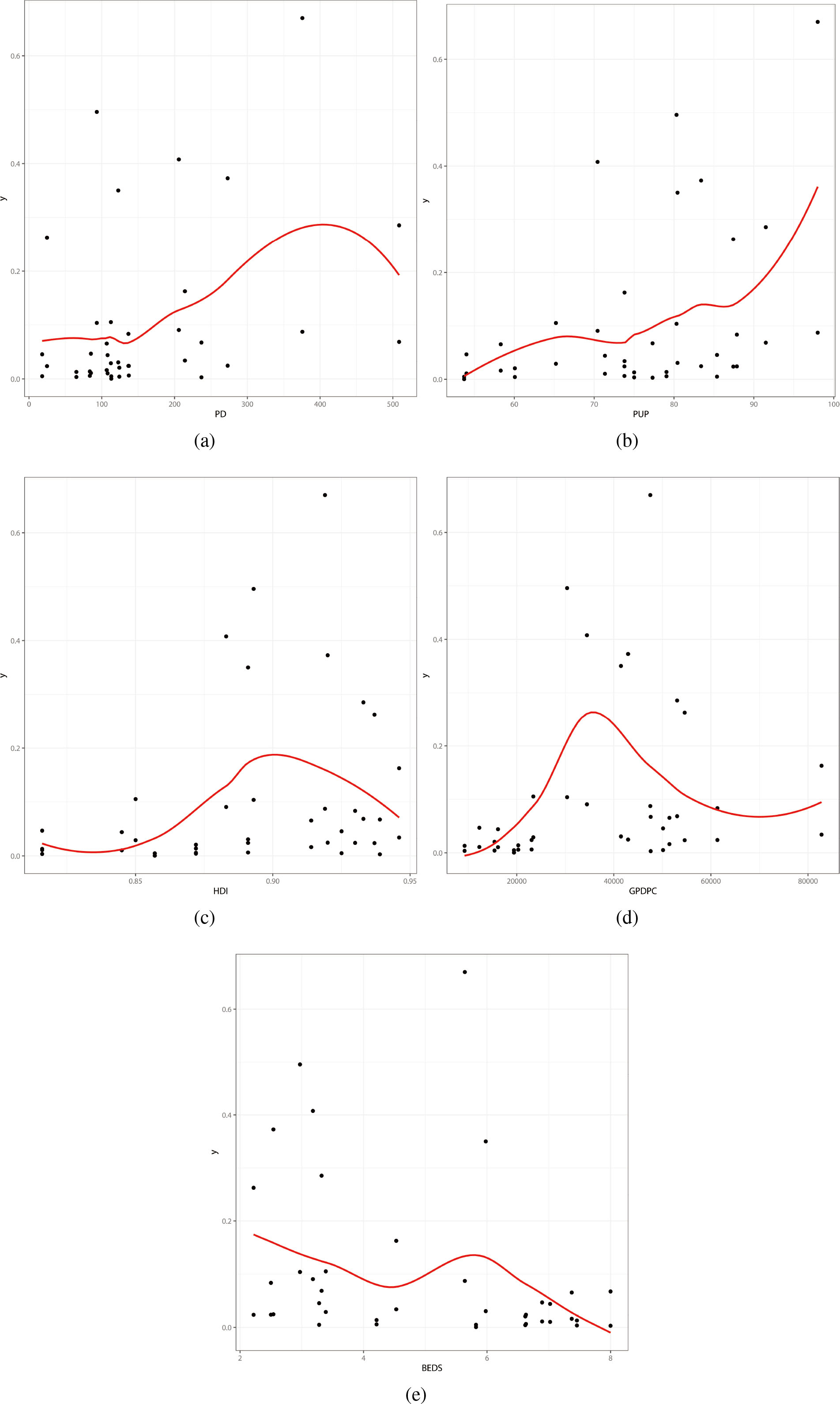
In particular, we provide some findings from the correlations of all variables reported in Table 2and Fig. 2.
• There is a discordant case corresponding to Belgium. This observation deviates the linear correlation between the response variable and some of the covariates. We discuss this case in the influence analysis.
3.3Fitted regression
There are simple computer programs to fit several kinds of regressions. We use the RS algorithm as described by Rigby and Stasinopoulos (2005) and Stasinopoulos and Rigby (2007) for maximizing Eq. (3) for the beta regression with two systematic components.
Table 2
Correlations values
| y vs PD | y vs PUP | y vs HDI | y vs GDPPC | y vs BEDS |
| 0.36 | 0.39 | 0.25 | 0.22 |
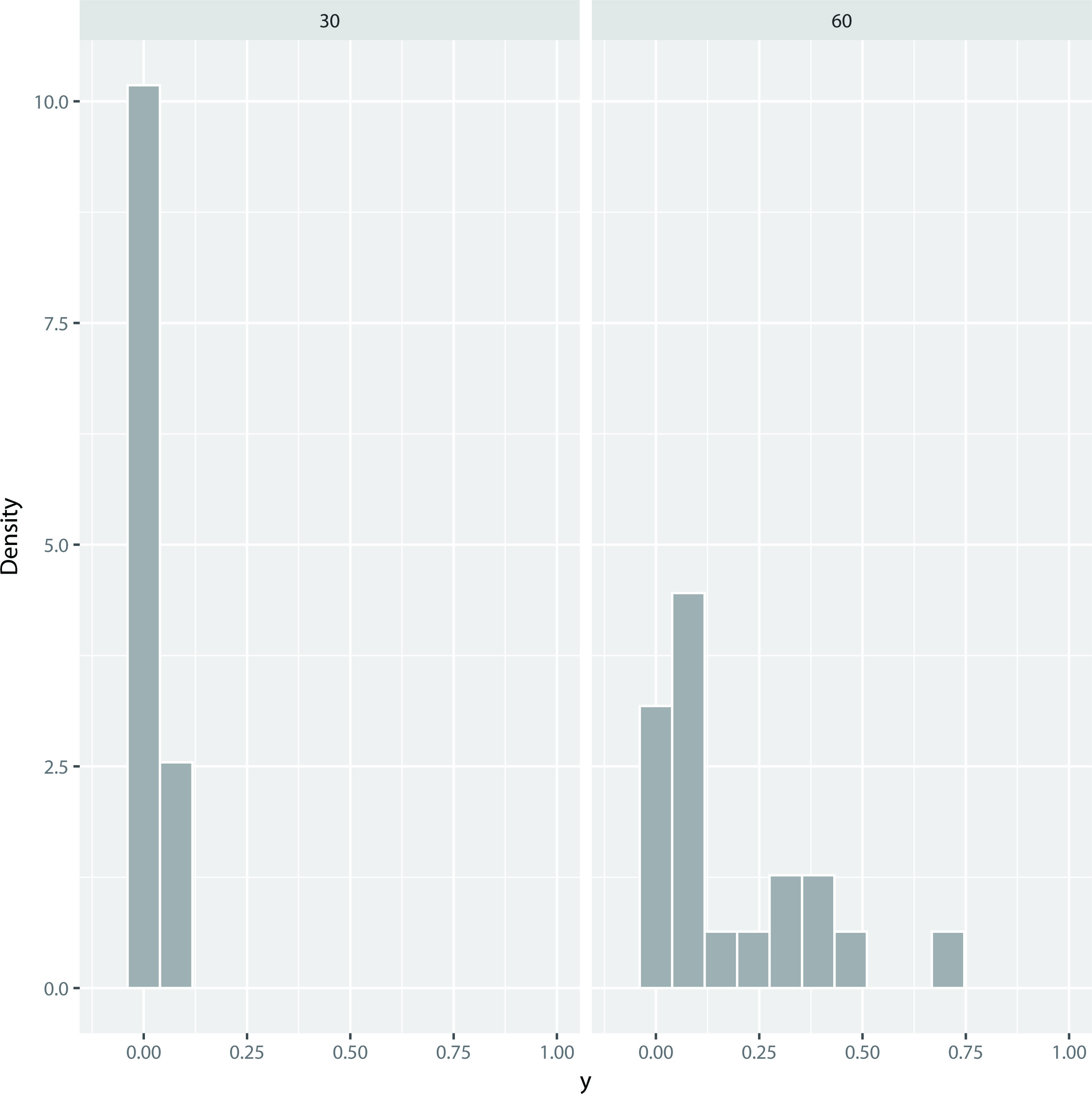
Figure 1.
Histograms of the mortality rate after 30 (MR (30)) and 60 (MR (60)) days.
The explanatory variables in the systematic components for the mean
Figure 2.
Dispersion Graphs. (a) y vs PD. (b) y vs PUP. (c) y vs HDI. (d) y vs GDPPC. (e) y vs BEDS.
The explanatory variables HDI and GDPPC are not significant for the mortality rates. Considering the variables PD, PUP, BEDS and TIME for both mean and dispersion parameters, the first two variables are not significant in the systematic component for the dispersion parameter. Therefore, the final systematic components for the beta regression can be expressed as
and
where
In the following, we shall compare the beta and simplex regressions. The simplex density defined by Barndorff-Nielsen and Jørgensen (1991) for a univariate continuous random variable
(4)
where
(5)
is the unit deviance. The systematic components for
We compare the fitted beta and simplex regressions using the global deviance (GD), Akaike information criterion (AIC) and Bayesian information criterion (BIC). These statistics in Table 3 indicate that the beta regression has lower values, and then it can be chosen as the best model to explain the coronavirus data.
Table 3
Statistics from the fitted regressions
| Model | GD | AIC | BIC |
|---|---|---|---|
| Beta | |||
| Simplex |
Next, a study of variable selection was carried out using the stepwise method in the beta regression in order to find a reduced model. Further, the MLEs of the parameters and their standard errors (SEs) and corresponding
Table 4
Results from the fitted beta regression to COVID-19 death rates
| MLE | SE | CI | ||
|---|---|---|---|---|
|
| ||||
| Intercept | 1.304 | ( | ||
| PD | 0.003 | 0.001 | (0.001, 0.005) | 0.007 |
| PUP | 0.027 | 0.014 | ( | 0.060 |
| BEDS | 0.088 | ( | 0.010 | |
| TIME | 0.070 | 0.009 | (0.0521, 0.088) | |
|
| ||||
| Intercept | 0.649 | ( | 0.0008 | |
| BEDS | 0.098 | ( | 0.085 | |
| TIME | 0.044 | 0.009 | (0.026, 0.062) |
Figure 3.
(a) Likelihood displacement. (b) Generalized Cook’s distance.
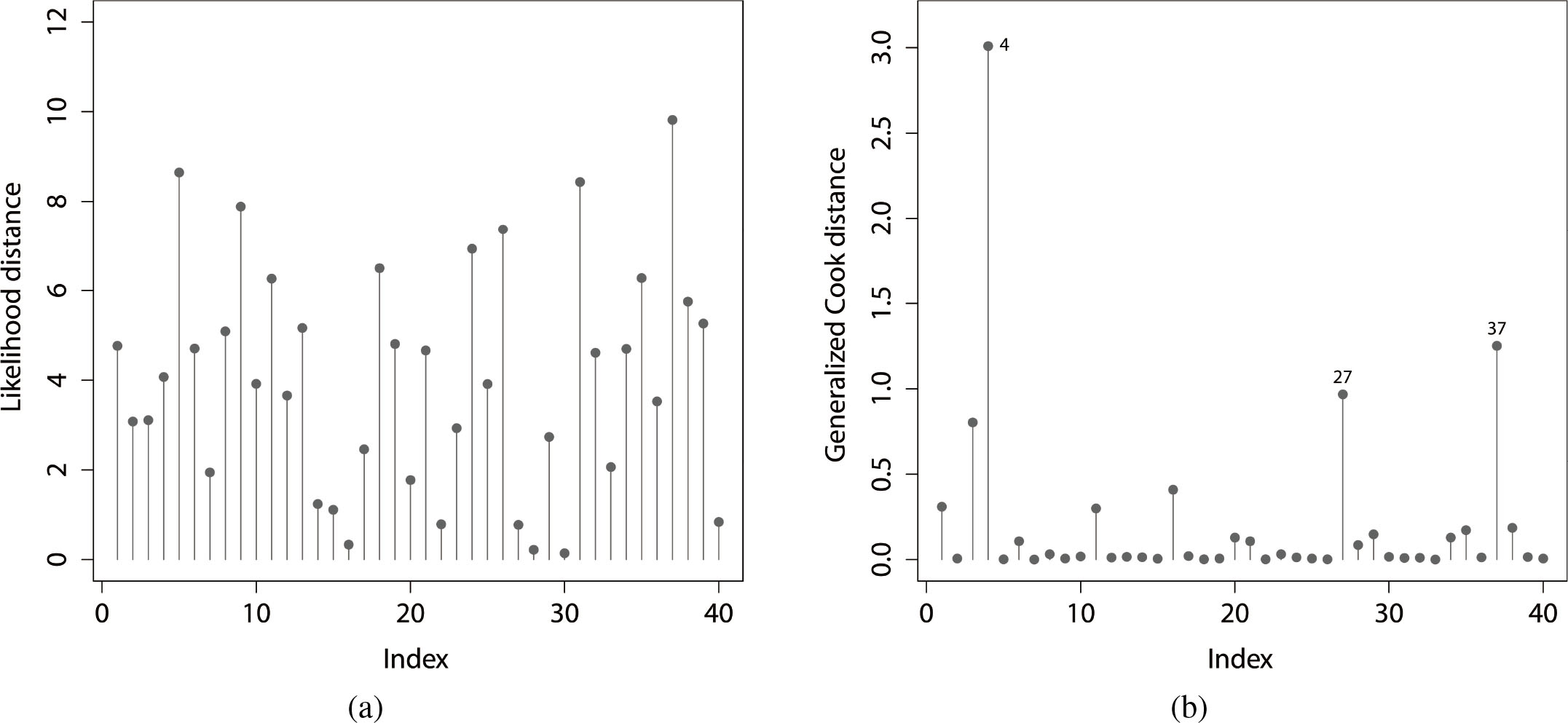
Influence analysis
The first tool to perform the sensitivity analysis called the global influence was introduced by Cook (1977). This method proposes the exclusion of cases to study the effect of the
where a quantity with subscript
An alternative measure to detect possible influential points is called the likelihood displacement
Figure 3 provides the plots of these measurements and the 4th observation is an influential case identified by
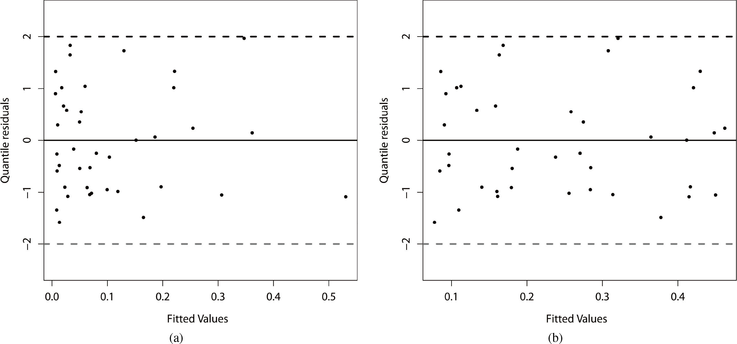
The plot of the residuals versus the adjusted values is displayed in Fig. 4 by considering the two systematic components. We can note that in the systematic component of the parameter
Figure 4.
Residual analysis of the beta regression model fitted to the current data. (a)
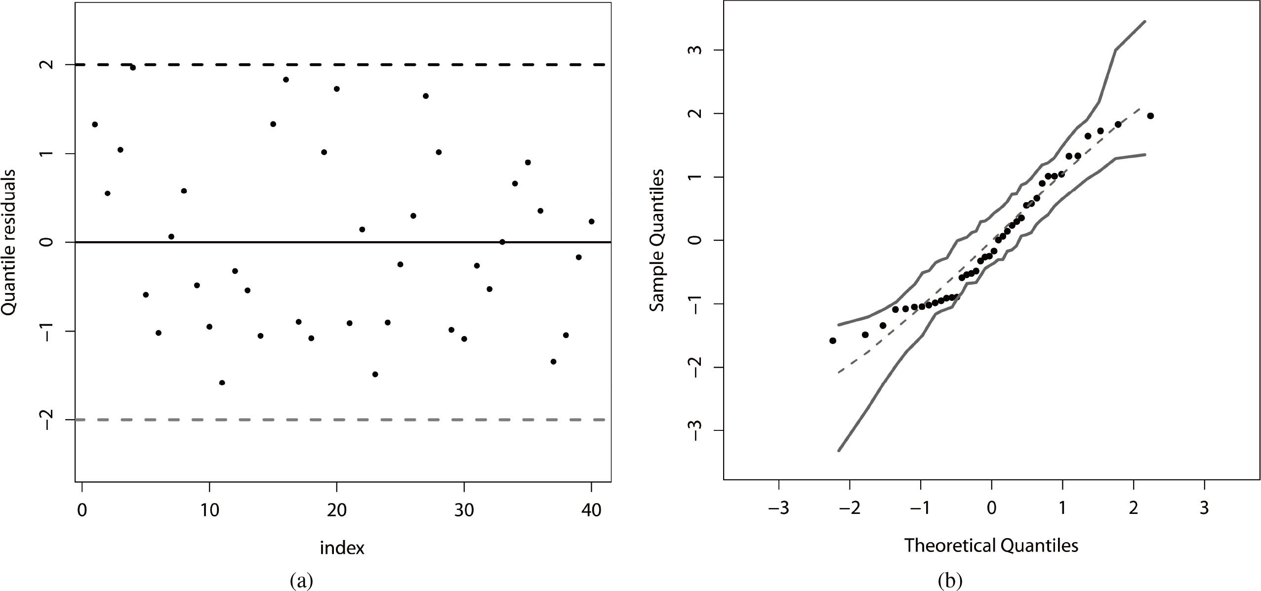
The plot of the quantile residuals (see Section 3.1) versus the order of the observations for the fitted beta regression is displayed in Fig. 5a, which indicates that the residuals are randomly distributed. Further, we verify the quality of the adjustment range of the fitted beta regression by constructing a simulated envelope. The plot in Fig. 5b reveals that there is strong evidence of a good fit of the beta regression to the current data. We can note that there are no discrepant observations. Thus, even Belgium is well fitted by the beta regression.
Figure 5.
(a) Quantile residuals. (b) Envelope for the quantile residuals.
The higher mortality rate in Belgium (one of the highest in the world) can be explained in great part for two facts outside our modeling: (i) the country has a global health security index (GHSI) lower than that of its neighbors. This indicator developed by the Johns Hopkins Center for Health Security assesses the overall protection capabilities of health systems worldwide. In order of safety, they appear: Netherlands
In the following, we present a brief summary of the results from the fitted beta regression with two systematic components defined before.
(iii)
(i) Findings from the systematic component for the parameter
– The population density is extremely significant (
– The percentage of the urban population is also significant for a significance level of 0.06. Thus, this mean mortality rate is higher for countries with large urban areas.
– The hospital beds proportion is very significant (
– Regarding the independent variable TIME which is highly significant (
In practical terms, the countries that have low proportions of hospital beds per 100 thousand inhabitants will have to increase their numbers of beds to cope with a future pandemic. Of course, the different public policies to control the pandemic adopted by countries are not including in our modeling.
The numbers of hospital beds are considered fixed for the beta and simplex regressions fitted to the mortality rates. There may have been small fluctuations in these numbers of beds during the studied periods. We did not have access to the fluctuations in the proportion of beds in the countries because this independent variable is supposed to be fixed in the proposed regressions. However, there is great complexity in studying these regressions with unit support for random explanatory variables, and we do not know of any theoretical involvement in this regard.
(ii) For the parameter
– The hospital beds proportion explains the dispersion of the mortality rate for a significance level of 0.10.
– Finally, there is a highly significant (
(iii) Marginal analysis from the estimated beta regression:
We can study the effects of the independent variables on the mortality rates marginally. The marginal effects of any independent variable (say
The last equation can be approximated by
4.Concluding remarks
COVID-19 is a disease caused by a new type of coronavirus first identified in Whuan (China) in December 2019. Most countries in West Europe started reporting cases of people infected at the end of February 2020. Confirmed cases across Europe had doubled over periods of three to four days, and even doubling every two days for some countries. The main objective of this article is to identify some demographic, socio-economic and health-care variables that explain the mortality rate in 20 countries in the fist wave in Western Europe using a beta regression with two systematic components. We identify that the population density, percentage of urban population, hospital beds per 100 thousand and during time explain significantly the mean and variability of the death rates in these countries.
Notes
3 World Health Organization. Considerations for quarantine of individuals in the context of containment for coronavirus disease (COVID-19). Geneva: World Health Organization; 2020. https://www.who.int/publications/i/item/considerations-for-quarantine-of-individuals-in-the- context-of-containment-for-coronavirus-disease-(covid-19).
4 Transmission of COVID-19 virus by droplets and aerosols: A critical review on the unresolved dichotomy https://www.ncbi.nlm.nih.gov/pmc/ articles/PMC7293495/.
5 Comorbidity and its Impact on Patients with COVID-19 https://www.ncbi.nlm.nih.gov/pmc/articles/PMC7314621/.
6 Comorbidities and the risk of severe or fatal outcomes associated with coronavirus disease 2019: A systematic review and meta-analysis https://www.sciencedirect.com/science/article/pii/S1201971220305725.
11 To get more information to UK response to COVID-19, see: https://www.gov.uk/coronavirus.
12 According to Bernucci et al. (2020), “this epidemic is challenging the Italian Government and the health care system and is having a devastating impact on all the health activities, including the neurosurgical reality”. See: https://www.wfns.org/WFNSData/Uploads/files/Effects-of-the-COVID-19-Outbreak-in-Northern-Italy-Perspectives-from-the-Bergamo-Neurosurgery-Department.pdf.
15 See: https://doi.org/10.1136/bmj.m2376.
References
[1] | According to Bernucci, et al. ((2020) ). This epidemic is challenging the Italian Government and the health care system and is having a devastating impact on all the health activities, including the neurosurgical reality. See: https://www.wfns.org/WFNSData/Uploads/files/Effects-of-the-COVID-19-Outbreak-in-Northern-Italy-Perspectives-from-the-Bergamo-Neurosurgery-Department.pdf. |
[2] | Atkinson, A. C. ((1985) ). Plots, transformations, and regression: An introduction to graphical methods of diagnostic regression analysis. Oxford: Clarendon Press Oxford. |
[3] | Barndorff-Nielsen, O. E. & Jørgensen, B. ((1991) ). Some parametric models on the simplex, Journal of Multivariate Analysis, 39: , 106-116. |
[4] | Bayer, F. M. & Cribari-Neto, F. ((2015) ). Bootstrap-based model selection criteria for beta regressions, Test, 24: , 776-795. |
[5] | Cook, R. D. ((1977) ). Detection of influential observation in linear regression, Technometrics, 19: , 15-18. |
[6] | Dunn, P. K. & Smyth, G. K. ((1996) ). Randomized quantile residuals, Journal of Computational and Graphical Statistics, 5: , 236-244. |
[7] | Ferrari, S. & Cribari-Neto, F. ((2004) ). Beta regression for modelling rates and proportions, Journal of Applied Statistics, 31: , 799-815. |
[8] | Guan, Y., Zheng, B. J., He, Y. Q., Liu, X. L., Zhuang, Z. X., Cheung, C. L., Luo, S. W., Li, P. H., Zhang, L. J., Guan, Y. J., Butt, K. M., Wong, K. L., Chan, K. W., Lim, Shortridge, W. K. F., Yuen, K. Y., Peiris, J. S. M. & Poon, L. L. M. ((2003) ). Isolation and characterization of viruses related to the SARS coronavirus from animals in Southern China, Science, 302: , 276-279. |
[9] | Haug, N., Geyrhofer, L., Londei, A., Dervic, E., Desvars-Larrive, A., Loreto, V., Pimior, B., Thurner, S. & Klimek, P. ((2020) ). Aerosol and surface stability of SARS-CoV-2 as compared with SARS-CoV-1, Nature Human Behaviour, 4: , 1303-1312. |
[10] | https://github.com/owid/covid-19-data/blob/master/public/data/README.md. |
[11] | Lauer, S. A., Grantz, K. H., Bi, Q., Jones, F. K., Zheng, Q., Meredith, H. R., Azman, A. S., Reich, N. G. & Lessler, J. ((2020) ). The incubation period of coronavirus disease 2019 (COVID-19) from publicly reported confirmed cases: Estimation and application, Annals of Internal Medicine, 172: , 577-582. |
[12] | Rigby, R. A. & Stasinopoulos, D. M. ((2005) ). Generalized additive models for location, scale and shape (with discussion), Applied Statistics, 54: , 507-554. |
[13] | Roser, M., Ritchie, H., Ortiz-Ospina, E. & Hasell, J. ((2020) ). Coronavirus pandemic (COVID-19), Published online at OurWorldInData.org. Retrieved from: https://covid.ourworldindata.org/data/owid-covid-data.csv. Accessed on 14 May 2020. |
[14] | See: https://arxiv.org/ftp/arxiv/papers/2003/2003.10518.pdf. |
[15] | |
[16] | |
[17] | |
[18] | |
[19] | |
[20] | |
[21] | See: https://www.thelancet.com/action/showPdf?pii=S0140-6736%2820%2930627-9. |
[22] | Stasinopoulos, D. M. & Rigby, R. A. ((2007) ). Generalized additive models for location scale and shape (GAMLSS) in R, Journal of Statistical Software, 23: , 1-46. |
[23] | To get more information to UK response to COVID-19, see: https://www.gov.uk/coronavirus. |
[24] | Tobías, A. ((2020) ). Evaluation of the lockdowns for the SARS-CoV-2 epidemic in Italy and Spain after one month follow up, Science of the Total Environment, 138-539. Retrieved from: https://www.sciencedirect.com/science/article/pii/S0048969720320520. Accessed on 30 July 2020. |
[25] | United Nations Development Program ((2019) ). 2019 Human development index ranking. Retrieved from: http://hdr.undp.org/en/content/2019-human-development-index-ranking. Accessed on 14 May 2020. |
[26] | United Nations, Department of Economic and Social Affairs, Population Division. ((2019) ). World urbanization prospects: The 2018 revision (ST/ESA/SER.A/420). New York: United Nations. Retrieved from: https://population.un.org/wup/Publications/Files/WUP2018-Report.pdf. Accessed on 14 May 2020. |
[27] | Van Doremalen, N., Morris, D. H., Holbrook, M. G., Gamble, A., Williamson, B. N., Tamin, A., Harcourt, J. L., Thornburg, N. J., Gerber, S. I., Lloyd-Smith, J. O., de Wit, E. & Munster, V. J. ((2020) ). Aerosol and surface stability of SARS-CoV-2 as compared with SARS-CoV-1, The New England Journal of Medicine, 382: , 1564-1567. |
[28] | Voudouris, V., Gilchrist, R., Rigby, R., Sedgwick, J. & Stasinopoulos, D. ((2012) ). Modelling skewness and kurtosis with the BCPE density in GAMLSS, Journal of Applied Statistics, 39: , 1279-1293. |
[29] | WorldBank ((2018) ). GDP per capita (current USS). Retrieved from: https://data.worldbank.org/indicator/NY.GDP.PCAP.CD. Accessed on 14 May 2020. |
[30] | Wu, D., Wu, T., Liu, Q. & Yang, Z. ((2020) ). The SARS-CoV-2 outbreak: What we know, International Journal of Infectious Diseases. Retrieved from: https://www.ijidonline.com/article/S1201-9712(20)30123-5/fulltext. Accessed on 30 June 2020. |

