Modelling the penumbra in Computed Tomography1
Abstract
BACKGROUND: In computed tomography (CT), the spot geometry is one of the main sources of error in CT images. Since X-rays do not arise from a point source, artefacts are produced. In particular there is a penumbra effect, leading to poorly defined edges within a reconstructed volume. Penumbra models can be simulated given a fixed spot geometry and the known experimental setup.
OBJECTIVE: This paper proposes to use a penumbra model, derived from Beer’s law, both to confirm spot geometry from penumbra data, and to quantify blurring in the image.
METHODS: Two models for the spot geometry are considered; one consists of a single Gaussian spot, the other is a mixture model consisting of a Gaussian spot together with a larger uniform spot.
RESULTS: The model consisting of a single Gaussian spot has a poor fit at the boundary. The mixture model (which adds a larger uniform spot) exhibits a much improved fit. The parameters corresponding to the uniform spot are similar across all powers, and further experiments suggest that the uniform spot produces only soft X-rays of relatively low-energy.
CONCLUSIONS: Thus, the precision of radiographs can be estimated from the penumbra effect in the image. The use of a thin copper filter reduces the size of the effective penumbra.
1Introduction
X-ray computed tomography has long been used in the medical field as an imaging technique for patient diagnosis, but more recently is finding employment as an indispensable non-destructive testing technology in industry used for a variety of dimensional metrological purposes [8, 24, 28, 30]. A prerequisite for its full acceptance in this field is the development of a thorough quantitative understanding of the main sources of error, to provide the rationale for a series of standards for its intended use, based on general guidelines for its use which are already in circulation [3, 27].
Broadly speaking, errors in X-ray CT fall into five categories; geometric errors, measurement object factors, environmental issues, user parameter selection and equipment error. Geometric errors, resulting from equipment misalignment and incorrect determination of positions of source and detector, have been given significant attention because of their importance in dimensional metrology [7, 14]. In particular artefact evaluation and subsequent voxel rescaling methods have been researched extensively [5, 9, 15, 18, 22, 25].
Measurement object factors such as the material(s) and size have an influence on parameter selection and hence impact on the final image quality. Two notable effects are beam hardening and scattering. These have been investigated by a number of authors and reduced through a combination of scanning strategies and post-processing filters [10, 16, 17, 20, 26].
Equipment errors are fundamental causes of error but are less frequently explored. For example, the detector is based on a number of pixels behind a scintillator (with several variations of detail to include CCD and amorphous silicon based models). There will undoubtedly be pixel-to-pixel variations(and even dead pixels) that could affect image quality and while general performance statistics have been compiled [6] there have been no detailed studies. Furthermore, image accuracy is limited by the spatial resolution of the detector. Apart from fluctuations in the selected voltage and current, errors arising from the source include improper focusing of the electron beam, variation in the resulting spot geometry and potential scatter. A previous work evaluated the spot shape in a non-focused system [13] but we have not been able to trace equivalent investigations for focused systems in the literature.
There are two main types of X-ray sources used in X-ray CT, namely reflection targets and transmission targets. Interaction of electrons with the anode causes emission of X-rays, with the spectrum dependent on electron energy and material of the anode. The difference between the two types of target arises in the anode itself; a transmission target is perpendicular to the electron beam generating a cone of X-rays along the same direction, whereas a reflection target is positioned at an angle to the electron beam so that the cone of X-rays is generated in a different direction to the electronbeam.
Focusing the electron beam results in an X-ray spot instead of a point source. Hence when the X-rays interact with the object, and are then recorded by the detector, blurring in the image can be observed. This is most easily seen at the penumbra which is the blurring specifically at the edges of the object image. When the spot is small, the radiation effectively originates from a point source, thus the boundary of the image is very sharp, and hence the penumbra does not appear. In contrast, when the spot is large, the radiation path depends on the location in the spot from which it originates, causing the edges to be less well-defined, creating a large penumbra as seen in Figure 1. Typically the size of the spot, and hence of the penumbra, increases with the power of the electron beam. This leads to a trade-off: while it is clearly desirable to minimise the power to reduce this effect, it may not then be possible to achieve the desired penetration for a fixed exposure time. The extent of the penumbra clearly leads to undesirable effects from a computed tomography perspective, causing poorly defined edges within a reconstructed volume that are further compounded by the partial volume effect resulting from a discrete domain (caused by pixelisation effects).
In addition to X-rays generated from the spot, the existence of secondary X-rays generated elsewhere within the source has been noted by previous authors. This has been studied in rotating- anode reflection target sources used in medical imaging systems [2, 19] and more recently in a transmission target source [4]. Boone et al. [4] find that imaging a lead ball with a transmission source leads to a light halo based effect as a result of this secondary source. They model the secondary source using a uniform ring alongside the focal spot using trial and error to match simulations to real data, but do not directly quantify the resulting penumbra.
This paper investigates the extent of the penumbra effect for 2D radiographs with respect to a simple rod geometry. A quantitative description of raw data is presented with validation against a simple spot model. The model reveals the existence of an extension to the penumbra in this setup that has the potential to affect a variety of sources; but it is noted that a simple filtering strategy can reduce this extended penumbra, thus resulting in superior quality images.
2Modelling
The typical source/detector geometry is shown in horizontal section in Figure 2. In order to isolate the effects of noise from all information about the spot geometry derived from the decay curve of the penumbra, a model-fitting methodology is adopted. Theoretically, penumbra models can be simulated once experimental parameters are given and the spot geometry is determined. The right spot geometry would provide simulated penumbra models which would agree with penumbra in radiographs. Thus this approach consists of three main steps: 1) constructing the model, 2) finding the best estimate for the model parameters, 3) evaluation of the fit. Two models for the spot geometry will be considered; one consists of a single Gaussian spot, the other is a mixture model consisting of a Gaussian spot together with a larger uniform spot. Within the fitting process, using real radiographic projections, we also estimate the attenuation coefficient μ.
2.1Constructing the model
The model should be accurate, yet its evaluation should be computationally cheap. To this end, several simplifying assumptions are imposed. It is assumed that the X-ray spectrum is monochromatic, and that there is no absorption in air. Variability due to the detector or scatter is also ignored. Finally, it is assumed that the detector is unsaturated, which is to say, signal strength of the detector increases linearly with X-ray intensity. This implies that the proportion of X-rays which pass through the object to register on the detector is exp(- μL), where μ is the attenuation coefficient and L is the path length through the sample, as governed by Beer’s Law. Note that the anode heel effect is negligible at the source-detector distance used.
Fix points O1 and O2 to be the feet of the perpendiculars from the centre of the cylinder onto the source line and detector respectively, with
(1)
A complete derivation of the above equation can be found in the appendix. All models in this paper will contain a Gaussian spot with full width half maximum (FWHM) of Dg. This reflects the common assumption that the actual spot is Gaussian with FWHM in microns equal to the power of the source in watts (see for example Müller et al. [21]). Let the model Gaussian spot be centred at signed distance s units from O1 with FWHM Dg, and further let the background air intensity at the detector be N. Using Equation 1, the intensity at the point K (at signed distance k units from O2) would be
(2)
However, as will be seen in Section 4.1, models with this single spot alone will fail to produce good agreement with the actual radiographs. Hence, a mixture model of the Gaussian spot and a larger uniform spot is proposed. Let the model uniform spot be a disk with centre (x + y)/2 and diameter Du = y - x where y > x. Ignoring height issues, the disk can be projected onto a line segment, where each point of this line segment is weighted by the length of the projected chord. This implies that the intensity at point K (at signed distance k units from O2) would involve a weighted integral between x and y, and would thus be a mixture of Equation 2 and
(3)
It is important to note that the model has limitations. Bearing in mind the overall assumptions, although the model should be acceptable within the penumbra, it will break down in the middle of the cylinder because of beam hardening effects. Furthermore, this model conflates the two major sources of blurring in the radiographic image: namely, the penumbra effect and the spatial resolution of the detector. These combine to form an overall unsharpness U in the image [12, 29]:
(4)
(5)
Finally, the large improvement in the fit, as seen in Section 4.2, arises from a small difference in the tail of the model spot. The heavier tail in the mixture can only be seen after magnifying the tail, as is illustrated in Figure 3.
2.2Fitting the model
The model gives a prediction of the image given the following variables: attenuation coefficient μ, diameters Dg and Du and position of the cylinder and the spot. The non-linear least squares method (nls) in the freely available open-source statistics software package R is used to find the variables which produce an image closest to a given radiograph. This is an iterative process which first finds a new estimate by using a first order approximation centred around the previous estimate. This is followed by a convergence check. If the residuals are nearly orthogonal to the tangent space, this indicates that a critical point has been reached and thus the procedure is terminated by checking whether the ratio between the scaled length of the tangent plane component and the scaled length of the orthogonal component is less than a fixed convergence tolerance (otherwise the process of finding a new estimate is repeated). The statistical package nls in R sets this to a default value of 10-6.
Practical users of the nls method need to be aware of two modes of failure. Firstly, the linear problem above may not have full column rank, and thus standard methods will not work. In R, this raises an error described as ‘singular gradient matrix at initial parameter estimates’. This is avoided by choice of good starting parameters. Secondly, the algorithm may experience extreme slowdown as step size becomes very small. In R, one of the controls of the nls function is the size of the minimum step, and if the step size is too small, the algorithm halts and raises an error described as ‘step factor reduced below minFactor’. This could indicate that the model is parametrised badly. On the other hand, this may arise from the default choice of the convergence tolerance of 10-6 being too demanding. It is possible that that the final estimate is within the minimum step size from the optimal solution, and so is entirely adequate. Bates and Watts [1] argue that a convergence tolerance of 0.001, or 10-3 is sufficient as ‘any inferences will not be affected materially by the fact that the current parameter vector is less than 0.1% of the radius of the confidence region from the least squares point’. Setting the convergence tolerance to 10-3 would have the additional advantage of resulting in speediermodel fits.
In this particular case, nls with a convergence tolerance of 10-6 runs to completion without raising either error once good starting parameters are chosen. Equation (5) gives good initial estimates for Dg and Du. The magnification of the rod object can be determined directly from the experimental setup, and the position of the central axis of the rod is estimated using a simple least-squares technique.
3Experimental method
In this study a Nikon XT H 225/320 X-ray CT system was used to obtain raw data for evaluation of the penumbra effect. The system consisted of a 225kV reflection target micro-focus source and an amorphous silicon detector (XRD 1621 AN (Perkin Elmer)) based on an array of 2000 x 2000 pixels each of size 200μm. The source and the detector are separated by a distance of 877mm. For much of the subsequent analysis it will be convenient to use a single pixel as the unit of measure for distances.
The sample used for penumbra evaluation was a 3mm ceramic rod, selected because it leads to relatively high attenuation in comparison to plastic but producing a minimal amount of scatter compared to potential metallic materials. It was placed centrally on the manipulator in an approximately vertical alignment, and such that the magnification was x4.45 resulting in an equivalent pixel size of 44.94(
4Results
As alluded to in the previous section, the model with a single spot alone does not give good agreement with any radiographs, whereas the mixture model provides a more reliable fit. For exposition purposes, this is demonstrated by examining the fit of one sample radiograph, seen in Figure 4 above; see Sections 4.1 (for single spot model) and 4.2 (for double spot model). This radiograph is taken with a power setting of 14.6 W, therefore the expected spot size would be 0.073 pixels (14.6μm), and thus from Equation (5), the expected Dg would be 0.293 pixels. In both sections, the parameters for the best fitting model will be found. Since the model breaks down in the cylinder due to beam hardening effects, the cylinder is ignored when judging goodness of fit. Instead, the boxed areas shown in Figure 4 are examined to test the model. Here the residuals, the difference between the model and the actual data, are considered. If the residuals are similar to white noise, then the model is considered to yield a good fit. Finally, the parameter fits in the mixture model are analysed in Section 4.3.
4.1Model fitting using a single Gaussian spot
The single Gaussian spot model, as indicated by Equation (2), is fitted to Figure 4 using nls as outlined in Section 2.2. Here, the best parameter fit for Dg is 0.77 pixels, which is much larger than the expected 0.293 pixels. The large model spot size is an artefact which arises because the fit is poor. This can be observed by examining the absolute residuals in Figure 5. The residuals of pixels within 40 pixels from the boundary (columns 870-910 and 1040-1080) averaged 620.4 (standard deviation = 498.4). In contrast, the residuals of pixels in the rest of the image averaged 75.9 (standard deviation = 365.7), which is much smaller. Therefore the model does not offer an adequate explanation of the data.
By trigonometry, if Dg were smaller than 2 pixels (400μm), then the intensities more than 9 pixels away from the boundary should be indistinguishable from air, as reflected in the model. However, this is not the case in the data. This can be best observed by looking at the raw data 5 to 75 pixels from the estimated cylinder boundaries, as plotted in Figure 6. As can be seen, the plot exhibits a gradient which is duplicated on both left and right sides of the image up to 40 pixels away from the boundary before flattening out at the mean grey level of air.
A natural explanation of this extended penumbra is that a second, more diffuse spot is producing a small but noticeable amount of X-rays. This is because the spot has to be larger than 2 pixels to have an effect on intensities more than 9 pixels away from the boundary. A relevant mixture model is noted by Dong et al. [11]: most of the X-rays come from a more concentrated spot but a small amount come from a larger region. This suggests a refinement of the previous one spot model to incorporate two spots.
4.2Model fitting using a mixture model
Here, a mixture is considered of the Gaussian spot, as indicated by Equation (2), and a secondary larger uniform spot, as indicated by Equation (3). The best parameter fit for the Du is 27.3 pixels (5450μm), that of Dg is 0.233 pixels, with the proportion of power in the outer spot being estimated at 4.3%. The value of Dg is thus much closer to the theoretical value of 0.293 pixels. Improvements can also be seen in the absolute residuals shown in Figure 7, measuring the difference between the model and the actual data. They have a mean value of 42.6, with standard deviation 371.8, with no patterns, thus resembling white noise. The residuals of pixels within 40 pixels from the boundary (columns 870-910 and 1040-1080) averaged 15.4 (standard deviation = 393.8). The residuals of pixels in the rest of the image averaged 56.2 (standard deviation = 362.9); the difference is much improved compared with the difference arising from the single-spot model. Therefore the extended model offers a better explanation of the data.
Since the residuals are similar to white noise, the fit provides an adequate explanation of the data. Thus, it remains to consider the actual parameter estimates from all the different radiographs.
4.3Parameter estimates
To ease computation, only rows 750 to 1250 of each image are considered. The units are returned to more conventional units of millimetres and microns to present the results. The estimates of position of the cylinder are constant throughout all the images, as expected. The estimated attenuation coefficient varies only by ±5% over all experiments, whichever spot model is employed. Furthermore, in the mixture model fits, the proportion of power of the larger spot remains constant at 4%, and Du averages around 5.3 mm across all powers with maximal deviation of 20% (see Figure 8). The values of Dg also do not deviate much from the theoretical unsharpness calculation referred to in Figure 9.
5Discussion
The amount of blurring present in an image depends directly on the spot geometry. The spot geometry is affected both by measurable factors, such as the electron beam fired at the source, as well as by unmeasurable sources of variation, such as ambient temperature and the pitting of the source. Consequently, the spot geometry may fluctuate from scan to scan. Any attempt to measure the spot geometry can only serve as a guide to the conditions in any subsequent experiments. Thus, it is best to have a way of measuring the spot geometry of an image by analysing the image itself.
The model detailed above delivers some success in this task. It is robust enough that the parameter estimates are consistent between iterates of the fitting algorithm nls. In particular, the consistency in the fitted attenuation coefficient implies that the monochromatic assumption has negligible effect on the model. Furthermore, each model contains a small Gaussian spot, with size similar to the theoretical unsharpness calculation in Equation (5), and corresponding to most of the power. Thus, the model corroborates results obtained with other commonly used models. On the other hand, the abnormally large penumbra cannot be explained as an artefact of the monochromatic assumption because this assumption only affects the intensities within the penumbra, and cannot affect the size of the penumbra. Hence, the model also shows something new –the existence of a larger uniform spot.
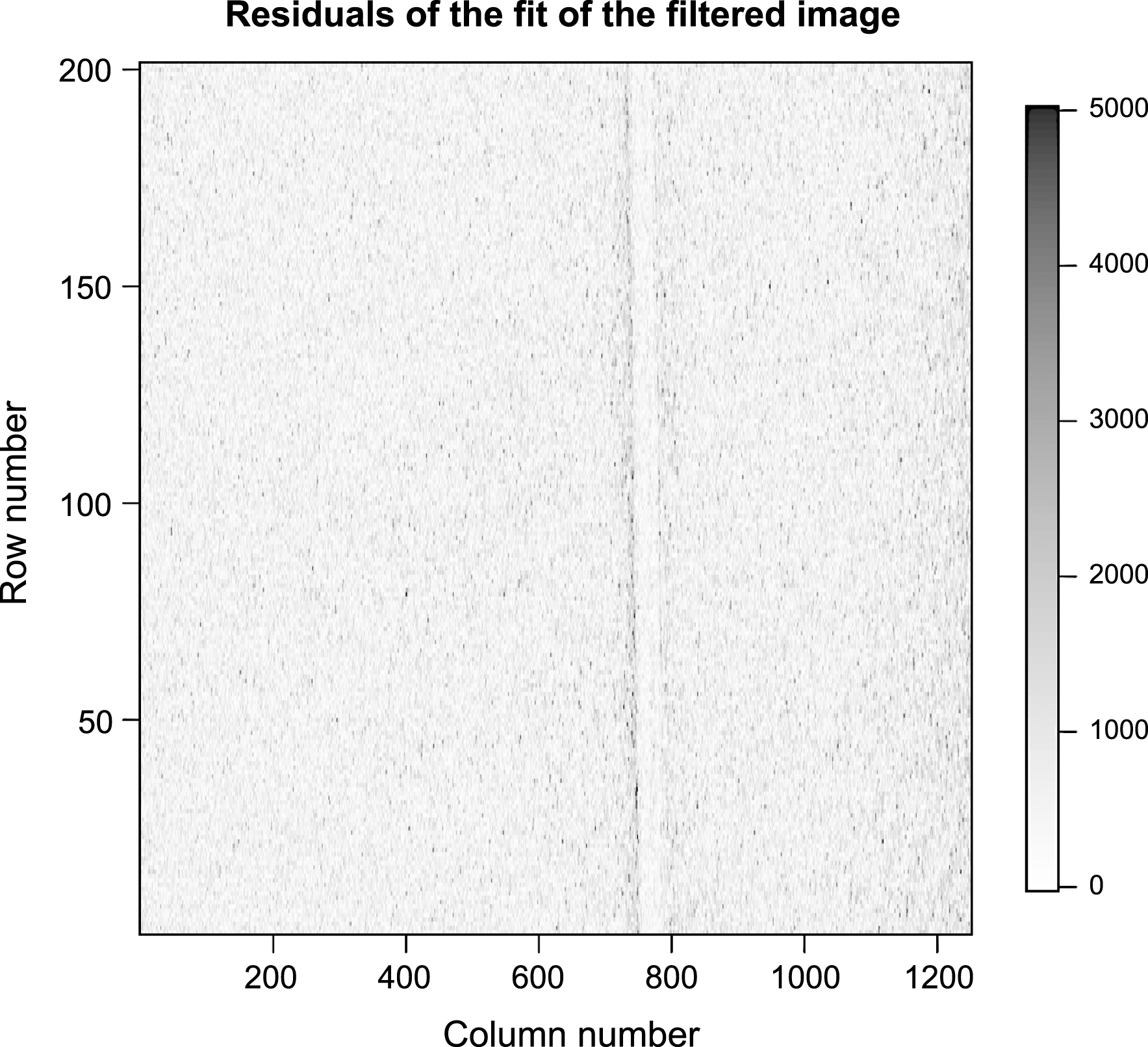
High magnification increases the size of the penumbra. To demonstrate the effect of this larger uniform spot, images of bent wire at approximately 50x magnification are considered. A straight section of wire is considered and the resulting image is used to fit the single Gaussian spot model. As expected, the residuals depart from the pattern expected of white noise (see in Figure 10). On the left, the classic penumbra, where pixels further from the object have lower residuals, is seen. On the right, there is no clear penumbra image because there is more wire in column 1400 outside the image which produces a mixture of penumbra.
For comparison, consider images taken using a thin copper pre-filter, but otherwise following the exact same process. The residuals of the fit now look much more like those we would expect of white noise, as shown in Figure 11. The thin copper filter, which removes low energy X-rays, reduces the failure of the fit and the effect of the unwanted larger spot.
This is strong evidence for supposing that the larger spot corresponds to soft X-rays of relatively low-energy. This supports the conjecture that this outer spot arises from X-ray scatter within the source tubing1
6Conclusion
It is important to evaluate the precision of radiographs when making inferences from CT images, which requires knowledge of the fluctuating spot geometry. In this work, the precision of radiographs has been estimated from the penumbra effect in the image. This shows that it is possible to confirm spot geometry from penumbra data, as well as to quantify blurring in the image. This work has also found evidence that although most X-rays are emitted from a small Gaussian spot, a small proportion ofX-rays come from a larger uniform spot. As noted in the discussion, the effect of the larger spot is reduced by interposing a thin copper filter at the source, suggesting that these X-rays are relatively low-energy. The size of this spot does not correlate with the direct anode interaction and spot generation, leading to the conclusion that there must be some internal scatter within the source that is emitted in all directions, limited only by the diameter of the window of the source itself, thus supporting the conjecture. Boone et al. [4] demonstrate the same effect in a transmission source geometry. We extend in a reflection target system, and then quantify the magnitude of the interference, modelling this by using a Gaussian spot/diffuse spot mixture.
Notes
1 This helpful conjecture was suggested by David Bate from Nikon Metrology during a site visit to Nikon UK on 10th July 2014. as has been found to exist in other source setups [2, 4, 19]. Variation in anode material should not affect the broad conclusion. For example, a molybdenum anode will lead to similar extended penumbra effects as the scatter within the source will still exist, resulting in an equivalent secondary spot, but with different intensity.
Appendices
Appendix A Derivation of Equation 1
By Beer’s Law, the proportion of X-rays which pass through the object from S to register on the detector at K is
(6)
Since the magnification is m,
(7)
Now, extend the line segment
(8)
Now, by the cosine rule,
(9)
Thus,
(10)
(11)
(12)
(13)
(14)
(15)
(16)
Putting it all together,
(17)
(18)
(19)
(20)
References
[1] | Bates D.M. and Watts. D.G. . Nonlinear Regression Analysis and Its Applications. John Wiley & Sons (1988) . |
[2] | Birch R. , The spectrum and intensity of extra-focal (off-focus) radiation. British Journal of Radiology 49: ((1976) ), 951–955. |
[3] | British Standards Institution, BS EN 16016 ((2011) ). |
[4] | Boone M.N. , Vlassenbroeck J. , Peetermans S. , Van Loo D. . Dierick M and Van Hoorebeke L, Secondary radiation in transmission-type x-ray tubes: Simulation, practical issues and solution in the context of x-ray microtomography. Nuclear Instrumentation Methods Physics Research Section A 661: ((2012) ), 7–12. |
[5] | Carmignato S. , Accuracy of industrial computed tomography measurements: Experimental results from an international comparison. CIRP Annals - Manufacturing Technology 61: ((2012) ), 491–494. |
[6] | Caruso D. , Dinsmore M. and Cornaby S. , Minature X-ray sources and the effects of spot size on system performance, International Centre for Diffraction Data ISSN 1097–0002 ((2010) ). |
[7] | Cho Y. , Moseley D.J. , Siewerdsen J.H. and Jaffray D.A. , Accurate technique for complete geometric calibration of cone-beam computed tomography systems. Medical Physics 32: ((2005) ), 968–983. |
[8] | De Chiffre L. . Carmignato S., Kruth J.-P and Schmitt R, Weckenmann A., Industrial applications of computed tomography. CIRP Annals - Manufacturing Technology 63: ((2014) ), 655–677. |
[9] | DeWulf W. , Kiekens K. , Tan Y. , Welkenhuyzen F. and Kruth J.-P. , Uncertainty determination and quantification for dimensional measurements with industrial computed tomography. CIRP Annals - Manufacturing Technology 62: ((2013) ), 535–538. |
[10] | DeWulf W. , Tan Y. and Kiekens K. , Sense and non-sense of beam hardening correction in CT metrology. CIRP Annals - Manufacturing Technology 61: ((2012) ), 495–498. |
[11] | Dong X. , Niu T. , Jia X. and Zhu L. , Relationship between X-ray illumination field size and flat field intensity and its impacts on X-ray imaging. Medical Physics 39: ((2012) ), 5901–5909. |
[12] | Dowsett D. , Kenny P.A. and Johnston R.E. , The Physics of Diagnostic Imaging, CRC Press, ((2006) ), 346. |
[13] | Gruner S.M. , Eikenberry E.F. and Tate M.W. , Comparison of X-ray detectors, International Tables for Crystallography Volume F: Crystallography of biological macromolecules, ((2001) ), 143–147. |
[14] | Kumar J. , Attridge A. , Wood P.K.C. and Williams M.A. , Analysis of the effect of cone-beam geometry and test object configuration on the measurement accuracy of a computed tomography scanner used for dimensional measurement. Measurement Science and Technology 22: ((2011) ), 035105. |
[15] | Leonard F. , Brown S.B. , Withers P.J. , Mummery P.M. and McCarthy M.B. , A new method of performance verification for x-ray computed tomography measurements. Measurement Science and Technology 25: ((2014) ), 065401. |
[16] | Li M. , Zheng J. , Zhang T. , Guan Y. , Xu P. and Sun M. , A prior-based metal artefact deduction algorithm for x-ray CT. Journal of X-Ray Science and Technology 23: ((2015) ), 229–241. |
[17] | Lifton J.J. , Malcolm A.A. and McBride J.W. , A simulation-based study on the influence of beam hardening in X-ray computed tomography for dimensional metrology. Journal of X-Ray Science and Technology 23: ((2015) ), 65–82. |
[18] | Lifton J.J. , Malcolm A.A. , McBride J.W. and Cross K.J. , The application of voxel size correction in X-ray computed tomography for dimensional metrology, Singapore International NDT Conference & Exhibition, ((2013) ). |
[19] | Miettunen R.H. , Measurement of extrafocal radiation by computed radiography. British Journal of Radiology 65: ((1992) ), 238–241. |
[20] | Mouton A. , Megherbi N. , Van Slambrouck K. , Nuyts J. and Breckon T.P, An experimental survey of metal artefact reduction in computed tomography. Journal of X-Ray Science and Technology 21: ((2013) ), 193–226. |
[21] | Müuller P. , Hiller J., Cantator A., Bartscher M. and DeChiffre L., Investigation on the influence of image quality in X-ray CT metrology. Conference on Industrial Computed Tomography, Wels, Austria ((2012) ), 229–238. |
[22] | Müuller P. , Hiller J., Dai Y, Andreasen J.L, Hansen H.N. and De Chiffre L., Estimation of measurement uncertainties in X-ray computed tomography metrology using the substitution method. CIRP Journal of Manufacturing Science and Technology 7: ((2014) ), 222–232. |
[23] | Russo P. and Mettivier G. , Method for measuring the focal spot size of an X-ray tube using a coded aperture mask and a digital detector. Medical Physics 38: ((2011) ), 2099–2115. |
[24] | Schick G. , Metrology CT technology and its applications in the precision engineering industry. Proceedings of SPIE 7522: ((2010) ), 75223S. |
[25] | Schmitt R. and Niggemann C. , Uncertainty in measurement for x-ray-computed tomography using calibrated work pieces. Measurement Science and Technology 21: ((2010) ), 054008. |
[26] | Siewerdsen J.H. and Jaffray D.A. , Cone-beam computed tomography with a flat-panel imager: Magnitude and effects of x-ray scatter. Medical Physics 28: ((2001) ), 220–231. |
[27] | Verein Deutscher Ingenieure, VDI/VDE 2630 ((2010) ). |
[28] | Weckenmann A. and Kramer P. , Computed tomography for application in manufacturing metrology. Key Engineering Materials 437: ((2010) ), 73–78. |
[29] | Weissleder R. , Molecular Imaging: Principles and Practice. People’s Medical Publishing House - USA ((2010) ), 59. |
[30] | Yancey R.N. , Eliasen D.S. , Gibson R. and Dzugan R. , CT-assisted metrology for manufacturing applications. Proceedings of SPIE 2948: ((1996) ), 222–231. |
Figures and Tables
Fig.1
The above plots show the varying intensity of rows in the spot model, which is introduced in Section 2, with two different spot sizes. The difference between the two is most pronounced in the penumbra, the blurring at the edge of the object image. When the spot size is small, the penumbra consists of gradient discontinuities; when the spot size is large, the penumbra is almost linear.
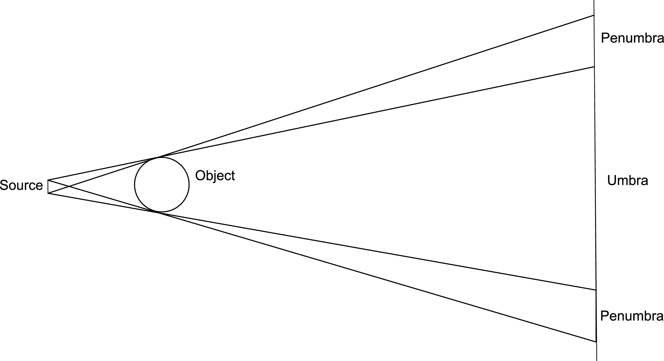
Fig.2
Horizontal cross-section of the experimental setup. A possible X-ray path from the source at point S to the detector at point K is shown.
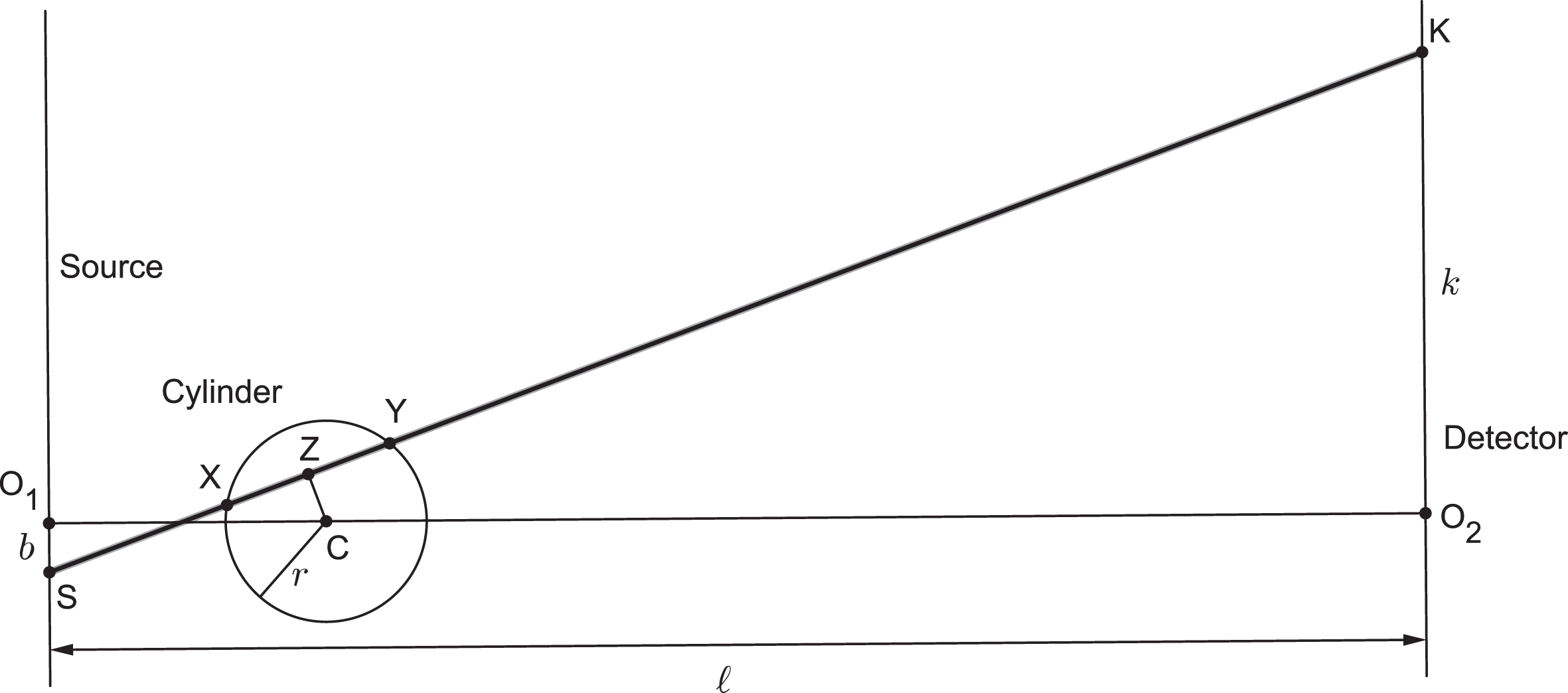
Fig.3
Tails from a single Gaussian spot (top) and the mixture of a Gaussian spot and the uniform spot (bottom). The heavier tails from the mixture can only be seen by magnifying the tail.
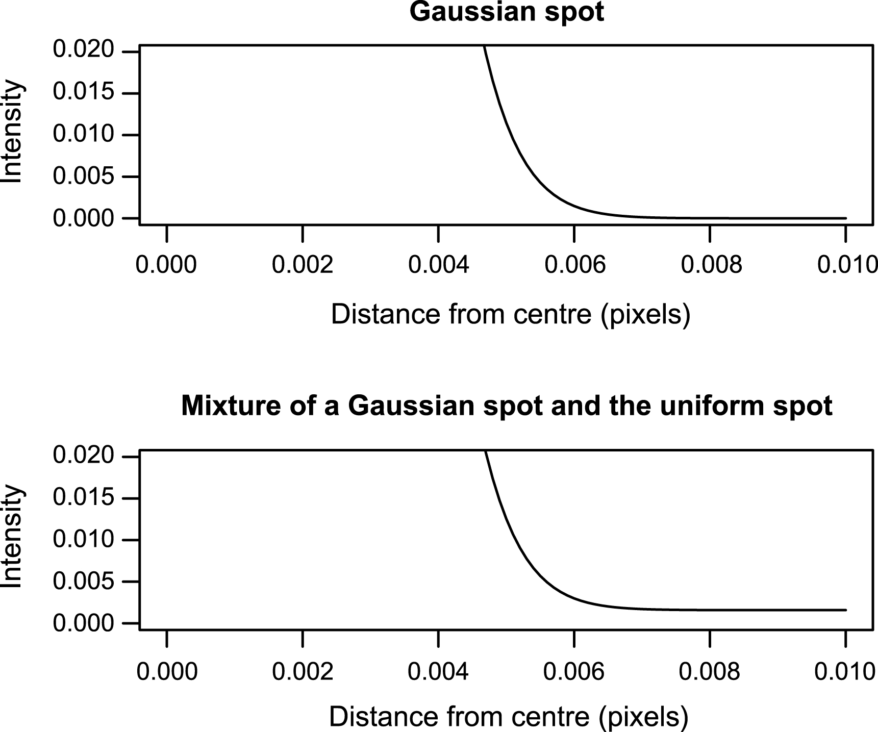
Fig.4
A sample radiograph, examined in depth in Sections 4.1 and 4.2. The dotted boxes to either side of the central cylinder profile indicate areas on the radiographs which are used to judge goodness of fit.
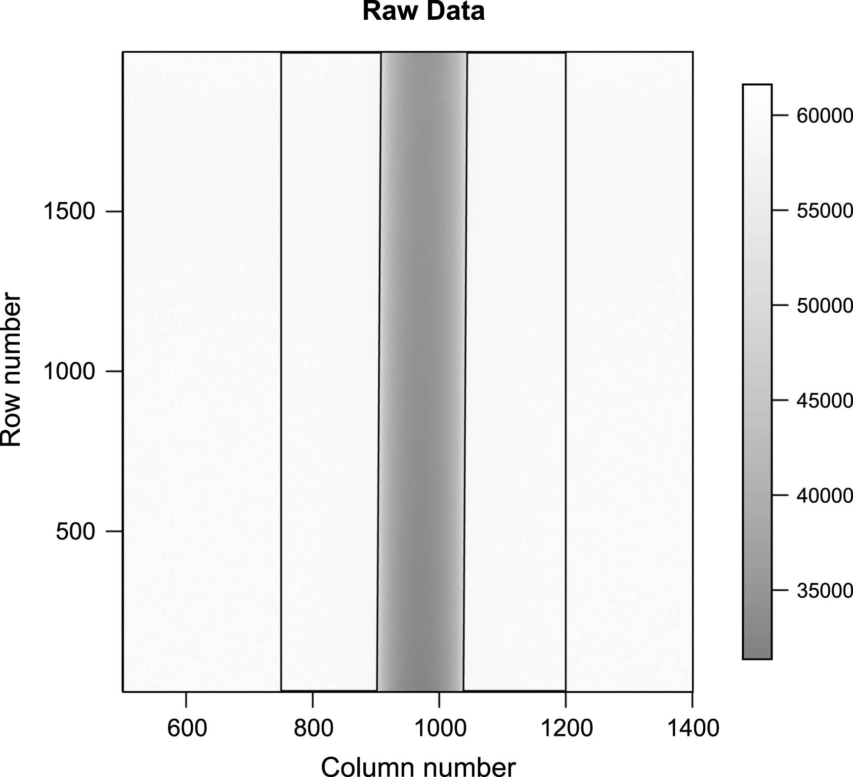
Fig.5
Absolute residuals of the single Gaussian spot model, as indicated by Equation (2). Absolute residuals are plotted so that larger residuals stand out. The residuals in close proximity to the cylinder found in columns 870-910 and 1040-1080 are high in absolute value compared to the rest of the image, thus the fit is poor.
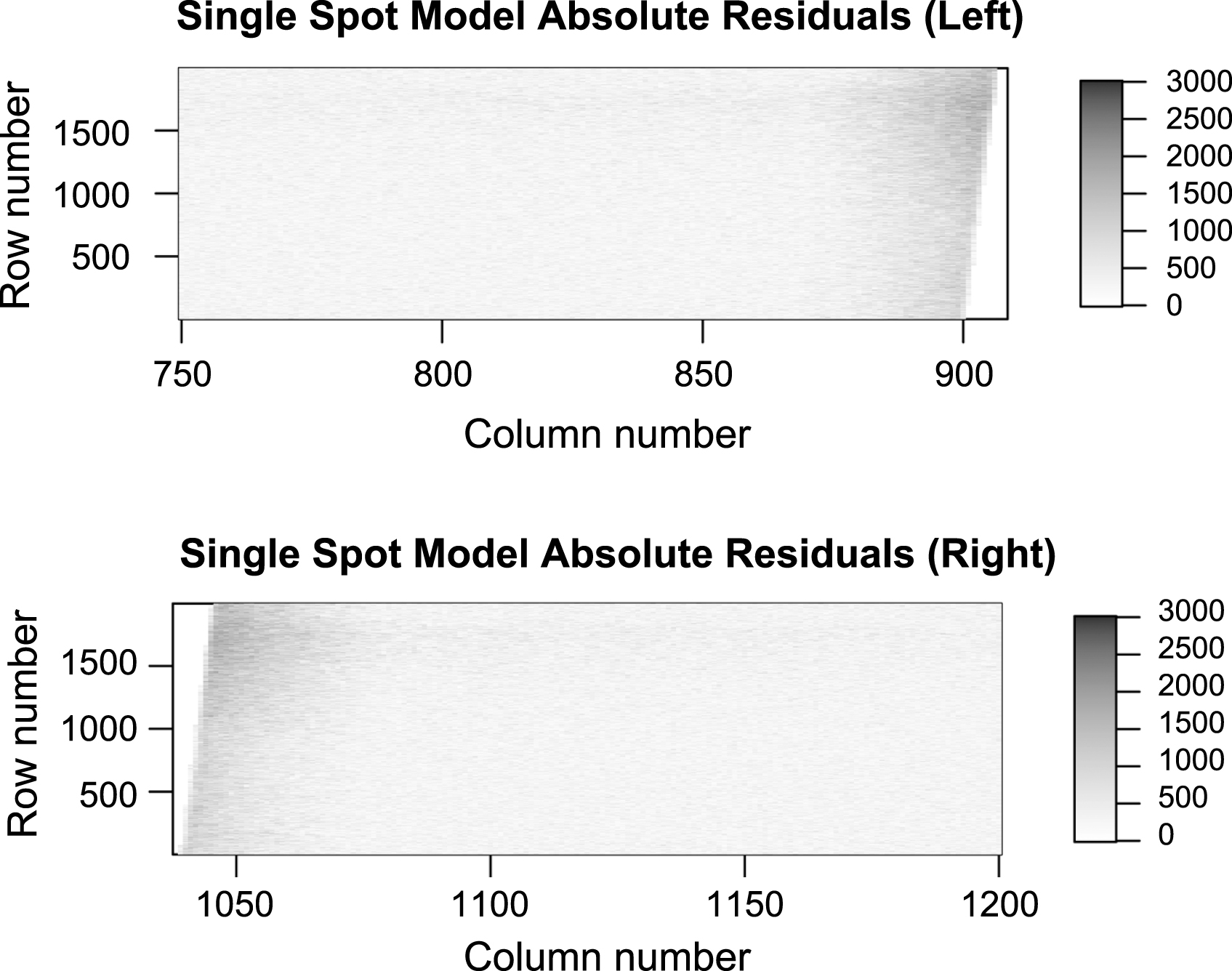
Fig.6
Raw data 5 to 75 pixels from the estimated boundaries of the cylinder in the whole image are adjusted for distance from the cylinder, and plotted here. The intensities flatten out at the mean grey level of air approximately 40 pixels from the boundary. This contradicts the single Gaussian model, which predicts that this would happen within 10 pixels from the boundary.
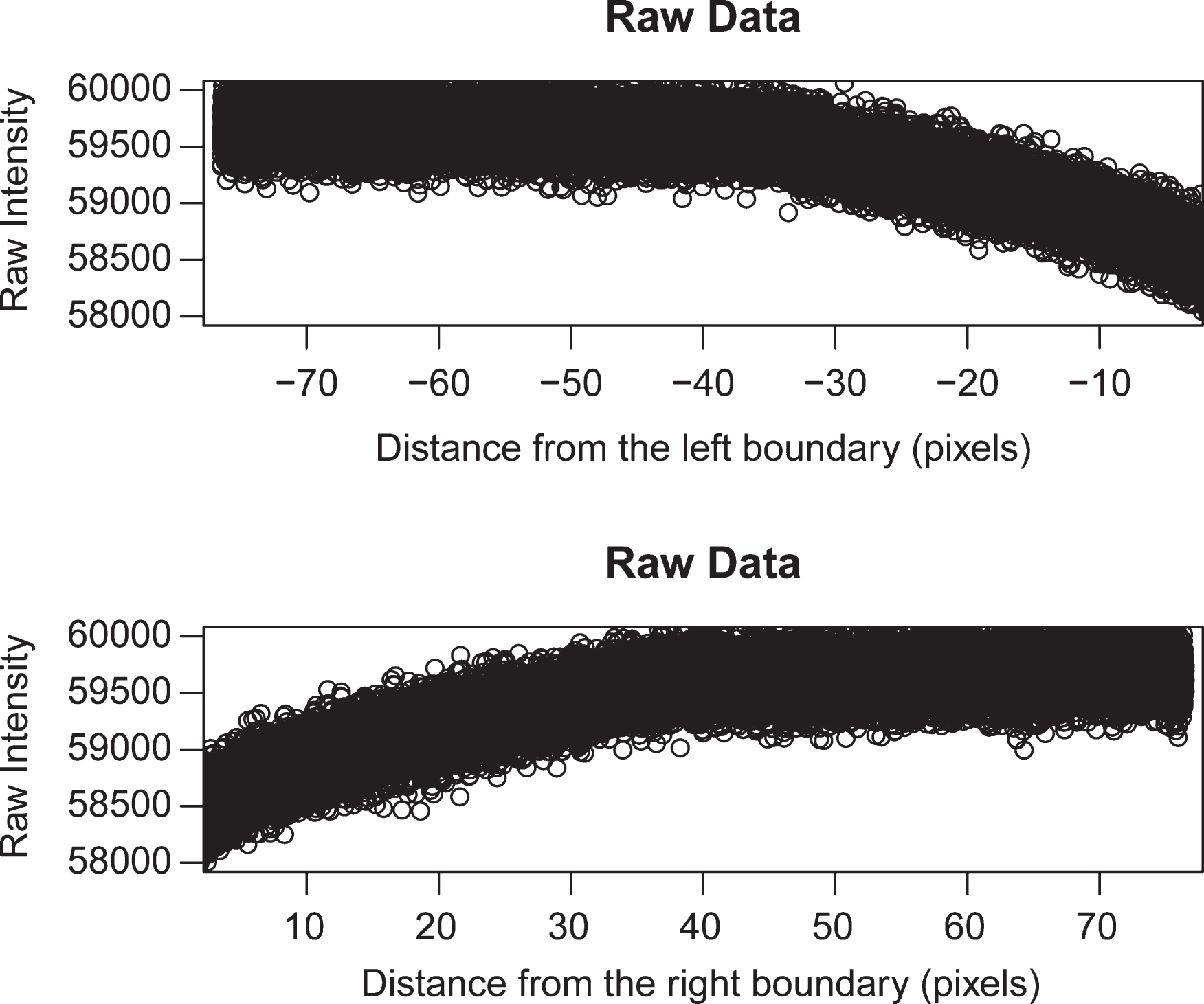
Fig.7
Absolute residuals of the mixture model. The residuals resemble white noise, so the model is adequate at explaining the data.
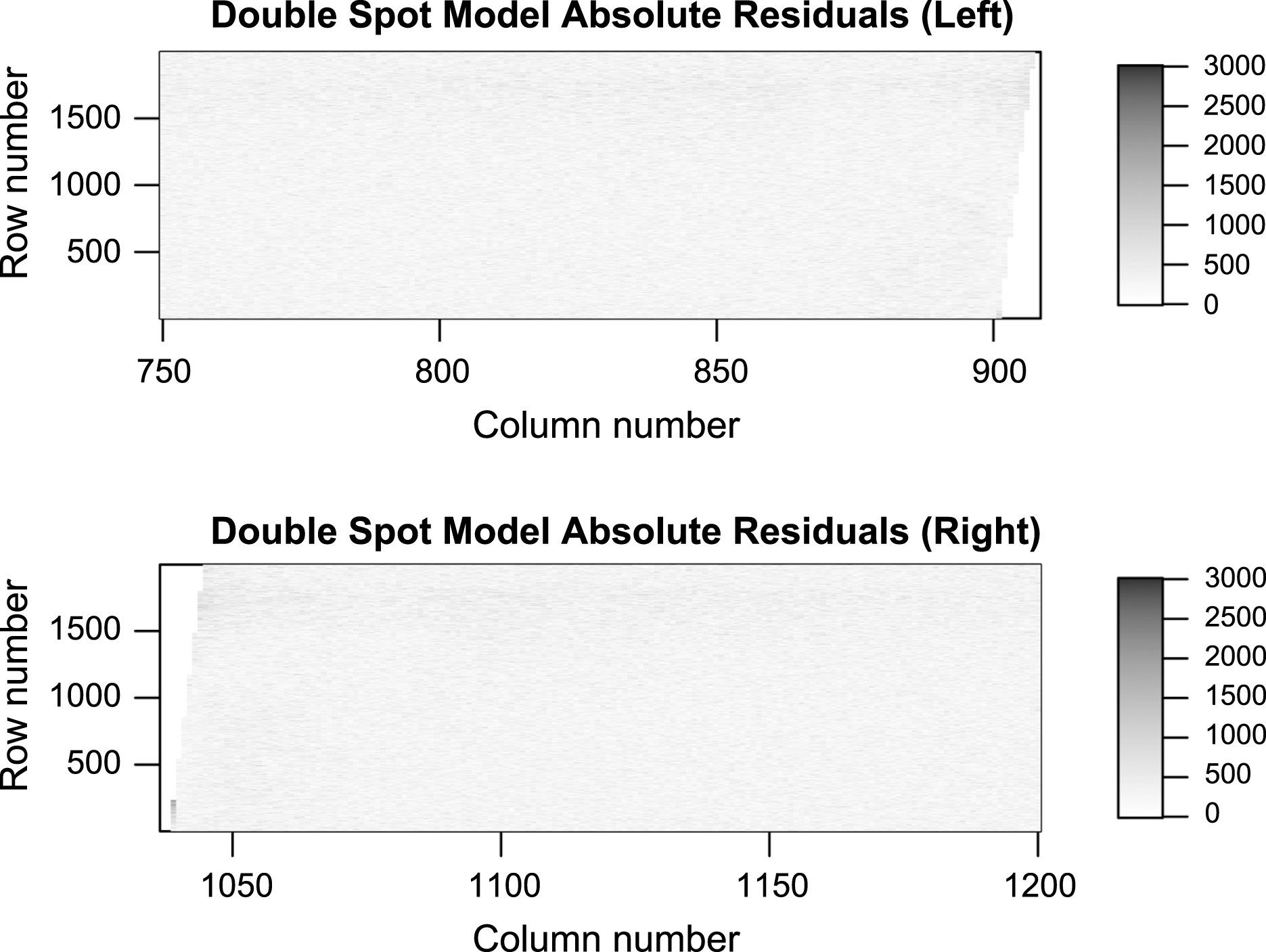
Fig.8
Properties of the model uniform spot when plotted against power. Note that they are broadly similar across all powers.
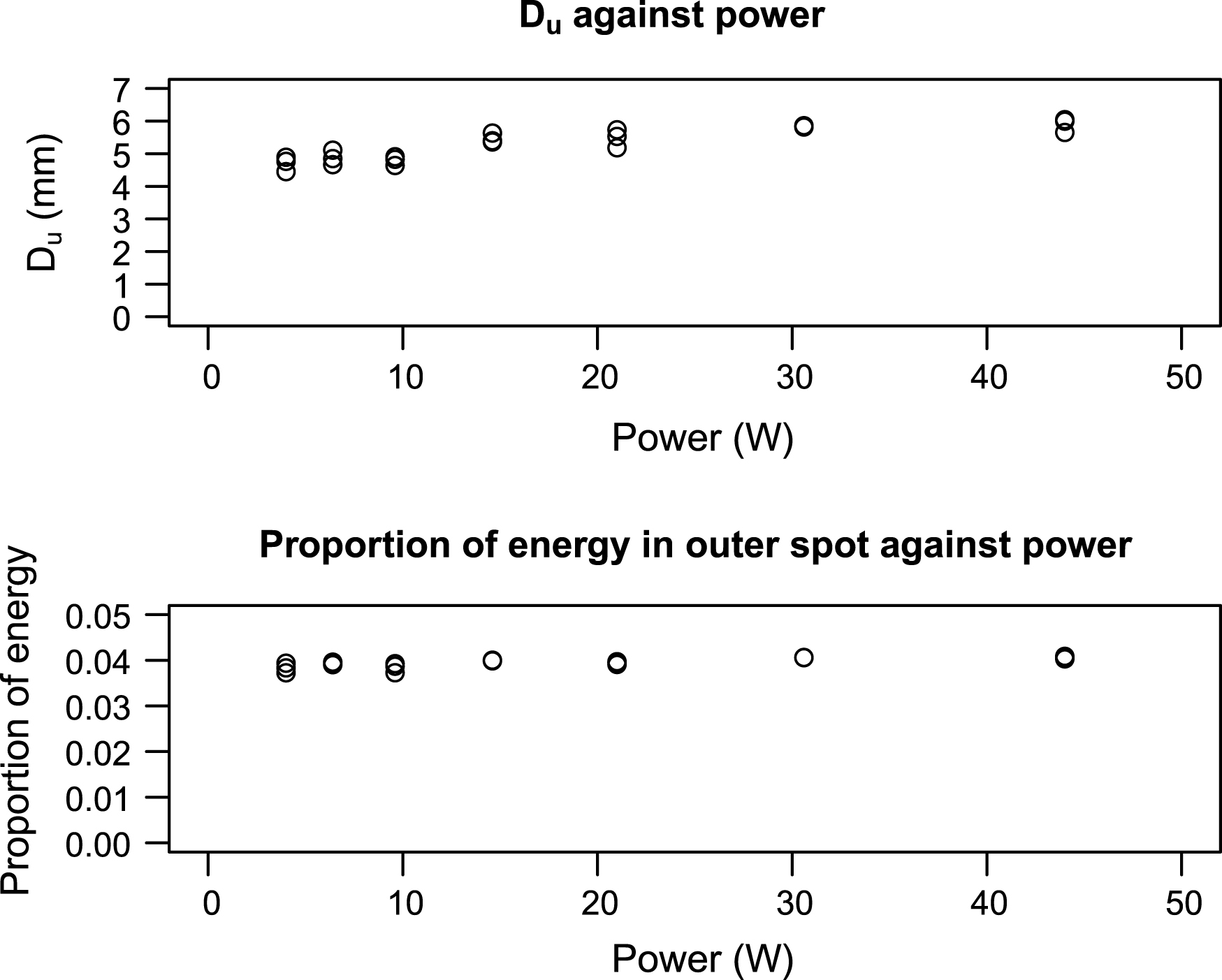
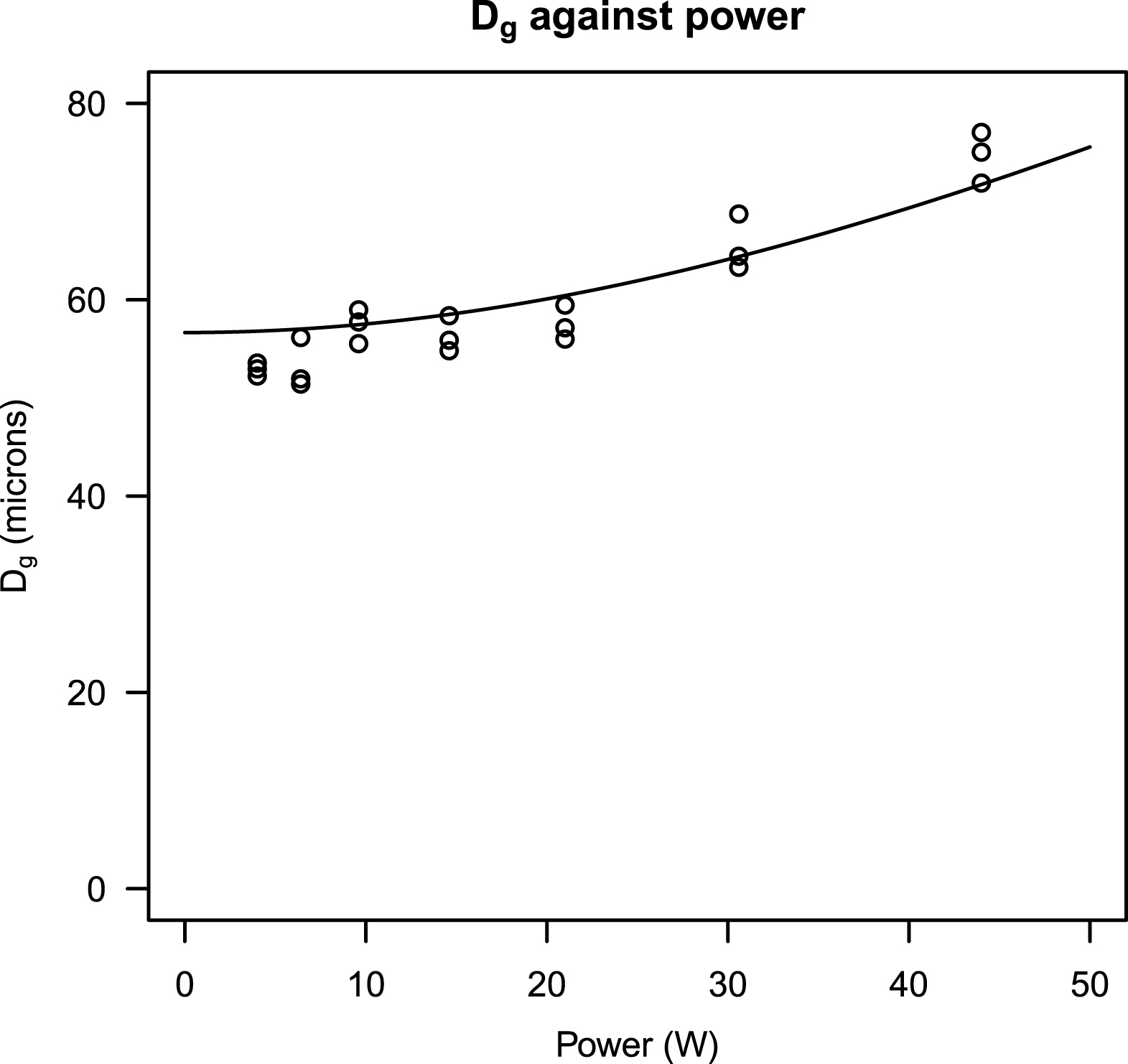
Fig.10
Absolute residuals of the single Gaussian spot model of the image. The residuals do not resemble those of white noise, thus the fit is inadequate.
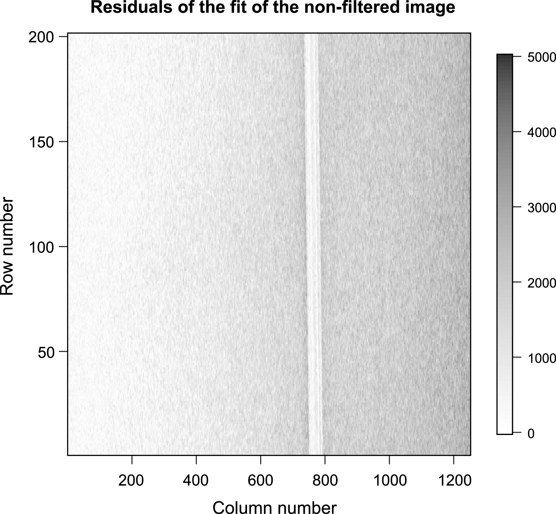
Fig.11
Absolute residuals of the single Gaussian spot model of the filtered image.