
Comparison of central, peripheral, and weighted size-specific dose in CT
Abstract
The objective of this study is to determine X-ray dose distribution and the correlation between central, peripheral and weighted-centre peripheral doses for various phantom sizes and tube voltages in computed tomography (CT). We used phantoms developed in-house, with various water-equivalent diameters (Dw) from 8.5 up to 42.1 cm. The phantoms have one hole in the centre and four holes at the periphery. By using these five holes, it is possible to measure the size-specific central dose (Ds,c), peripheral dose (Ds,p), and weighted dose (Ds,w).The phantoms are scanned using a CT scanner (Siemens Somatom Definition AS), with the tube voltage varied from 80 up to 140 kVps. The doses are measured using a pencil ionization chamber (Ray safe X2 CT Sensor) in every hole for all phantoms. The relationships between Ds,c, Ds,p, and Ds,w, and the water-equivalent diameter are established. The size-conversion factors are calculated. Comparisons between Ds,c, Ds,p, and Ds,ware also established. We observe that the dose is relatively homogeneous over the phantom for water-equivalent diameters of 12–14 cm. For water-equivalent diameters less than 12 cm, the dose in the centre is higher than at the periphery, whereas for water-equivalent diameters greater than 14 cm, the dose at the centre is lower than that at the periphery. We also find that the distribution of the doses is influenced by the tube voltage. These dose distributions may be useful for calculating organ doses for specific patients using their CT images in future clinical practice.
1Introduction
Although dosimetry of CT scanners began soon after the discovery of the CT scanner in the early 1970s [1], a method for the practical determination of CT output dose (CT dose index, CTDI) was only introduced about ten years later [2], and a method for the practical estimation of patient doses (the size-specific dose estimate, SSDE) was only introduced in 2011 by the American Association of Physicists in Medicine (AAPM) [3]. The magnitude of the SSDE is calculated based on the CT output dose in terms of volumetric CT dose index (CTDIvol), and the size-conversion factor (f) based on the effective diameter (Deff) [4]. AAPM has provided size-conversion factors, both for the head phantom (CTDIvol-16) and the body phantom (CTDIvol-32) [3]. In 2014, AAPM improved the SSDE concept by recommending the use of more robust expression of patient size, i.e. the water-equivalent diameter (Dw) [5]. In 2019, AAPM improved the size-conversion factor for the estimation of the patient’s head dose [6], so that a more accurate dose estimate could be obtained.
At present, the SSDE concept has been widely accepted [7–9] and is widely used for various applications, for example for radiation dose surveys [10], dose optimization [11–13], establishing diagnostic reference levels (DRL) [14, 15], and so on. Various attempts to improve SSDE calculations have been carried out [16, 17], and automation of these calculations to make them easier and more effective, are also now available [18, 19]. However, it should be underlined that the concept of SSDE is only an estimate of the average dose in patients delivered during a CT scan [20, 21]. The radiation dose inside the patient may not be homogeneous. Evaluation of radiation dose distributions using a PMMA phantom with a size of 32 cm (body phantom) reported that the dose in the centre of the phantom was much smaller than the dose at the periphery, and the difference between these dose was up to around 40% [22]. On the other hand, evaluation of the dose distribution with a PMMA phantom of size 16 cm (head phantom) reported that the radiation dose was relatively homogeneous, with the dose at the centre and the periphery relatively the same [23].
Evaluation of dose distribution for various phantom sizes has not been carried out yet. It is important to conduct a study on the dose distribution for various phantom sizes reflecting the variations between patients. An understanding of the dose distribution for different phantom sizes may be useful for calculating the dose to an organ at a specific position within a patient of a certain size [24]. Organ dose estimation has indeed been proposed using the SSDE concept [25], but it generally obtained using Monte Carlo simulations on various phantom models [26–28] or using anthropomorphic phantoms [29]. Direct organ dose calculation using the patient image is undergoing development and faces many challenges that need to be addressed [30].
Calculating organ doses directly from the patient image requires sufficient information about the patient dose and its distribution within the patient [31]. This study aims to determine and investigate the distribution of the dose within a phantom, and to determine the correlation between central, peripheral and weighted size-specific dose for various phantom sizes. Because the dose distribution may also be influenced by the tube voltage used, we also evaluated the dose distribution for the variation of the tube voltage that is commonly used in CT scanning.
2Method
2.1Phantom development
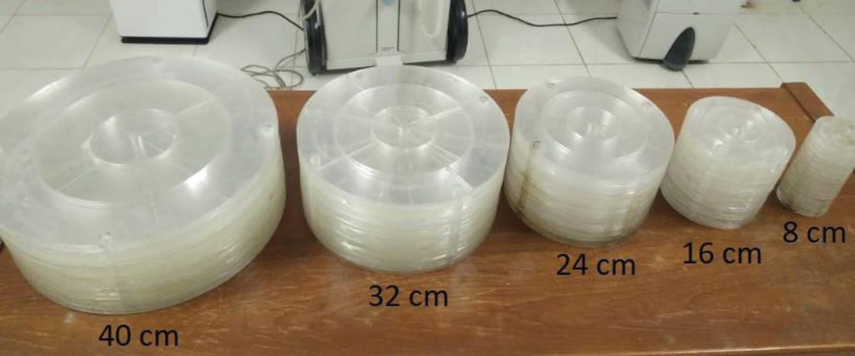
We used in-house phantoms with various physical diameters from 8 cm to 40 cm (Fig. 1), corresponding to the water-equivalent diameters from 8.5 to 42.1 cm. The phantoms were constructed from acrylic material corresponding to 123 Hounsfield units (HU) [32]. The phantoms had a hole in the centre and four holes equally spaced around the periphery, enabling the measurement of the size-specific central dose (Ds,c) and peripheral dose (Ds,p).
Fig. 1
In-house acrylic phantoms with various physical diameters from 8 cm up to 40 cm. The phantoms had four holes near the periphery and a hole in the centre allowing measurements of the size-specific peripheral dose (Ds,p) and the size-specific central dose (Ds,c).
2.2Dose measurement
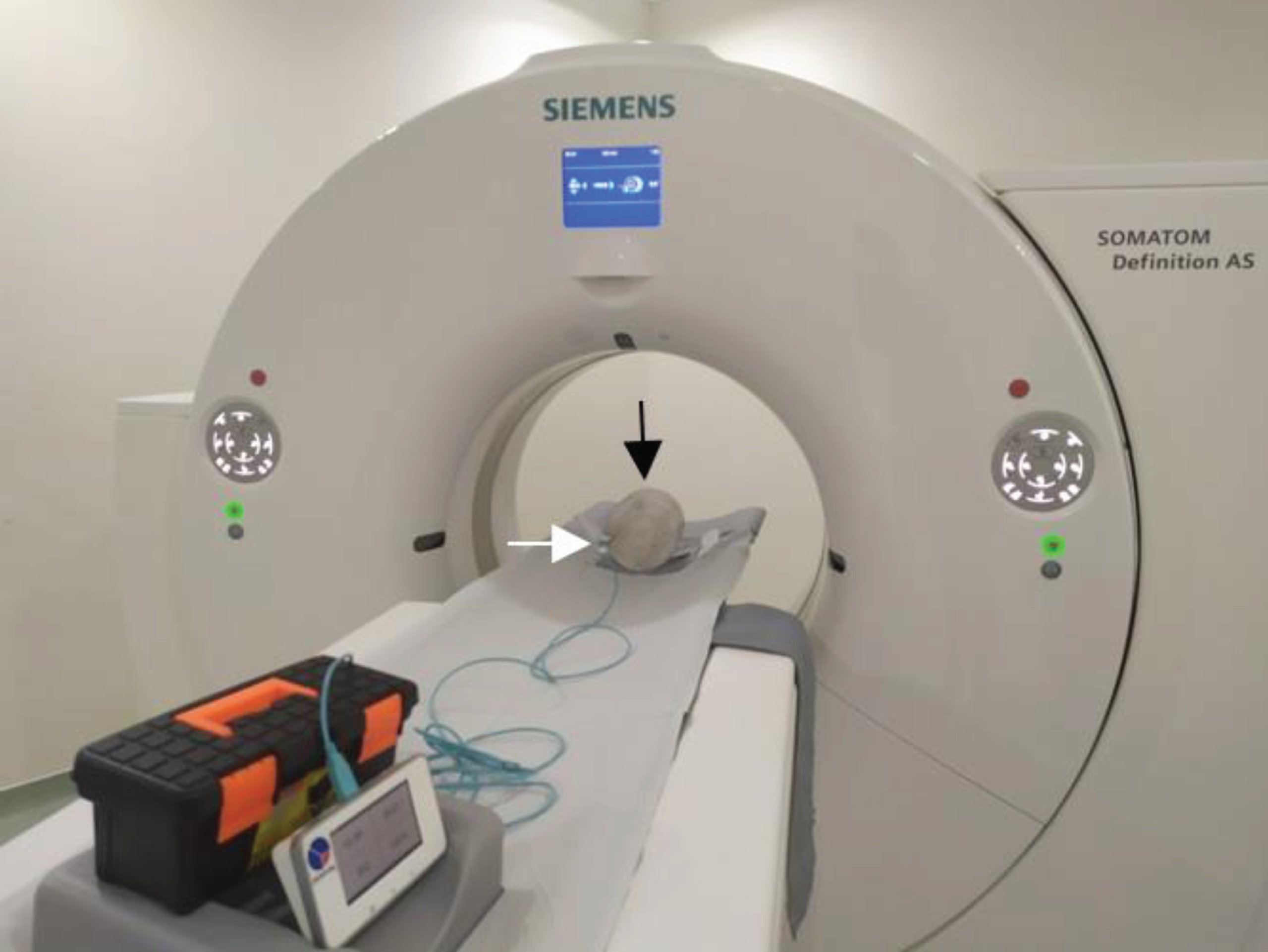
The phantoms were scanned using a CT Scanner (Siemens Somatom Definition AS). They were orientated so that the peripheral holes were orientated to be anterior, posterior, left and right. We used a body protocol with various tube voltages from 80 up to 140 kVps, a tube current-time of 200 mAs, and a slice thickness of 10 mm in one axial rotation. The doses were measured using a pencil ionization chamber (Raysafe X2 CT Sensor, Raysafe Inc., Billdal, Sweden) in every hole of all the phantoms. Figure 2 shows the 16 cm acrylic phantom on a patient table. A white arrow indicates the position of the pencil ionization chambers in one of the holes.
Fig. 2
Siemens Somatom Definition AS CT scanner. The black arrow shows a phantom with a diameter of 16 cm, and the white arrow shows the position of the pencil chamber on the periphery at a position of 9 o’clock.
For each phantom, the average Ds,p was calculated from four measurements:
(1)
The size-specific weighted dose (Ds,w) was calculated using Equation (2) in the same way as calculating weighted CTDI (CTDIw) [33]:
(2)
The relationship between Ds,w and the water-equivalent diameter (Dw) was established using an exponential regression (equation 3). The relationships between Ds,c and Dw, and Ds,p and Dw were established using third order polynomial regressions (equations 4 and 5).
(3)
(4)
(5)
The centre (fc), peripheral (fp), and weighted (fw) size-conversion factors were calculated.
(6)
(7)
(8)
The comparisons among Ds,c, Ds,p, and Ds,w were derived.
(9)
(10)
(11)
By using the previous relationships, the size-specific dose estimates for central (SSDEc), peripheral (SSDEp), and weighted (SSDEw) could be computed.
(12)
(13)
(14)
The CT console or Digital Imaging and Communications in Medicine (DICOM) header usually shows CTDIvol or dose-length product (DLP). For practical SSDE calculation, therefore, the CTDIw could be computed by using Equation (15).
(15)
The SSDEc and SSDEp could also be easily calculated using Equations (16) and (17)
(16)
(17)
It should be noted that Ds and SSDE are almost the same because they both show a dose at a certain size, but there is a slight difference. Ds is a measured dose in phantom of a certain size, while SSDE is the estimated dose in patients of a certain size as a result of calculations using the size-conversion factor (f) and volumetric CTDI (CTDIvol).
3Results
3.1Regression of dose
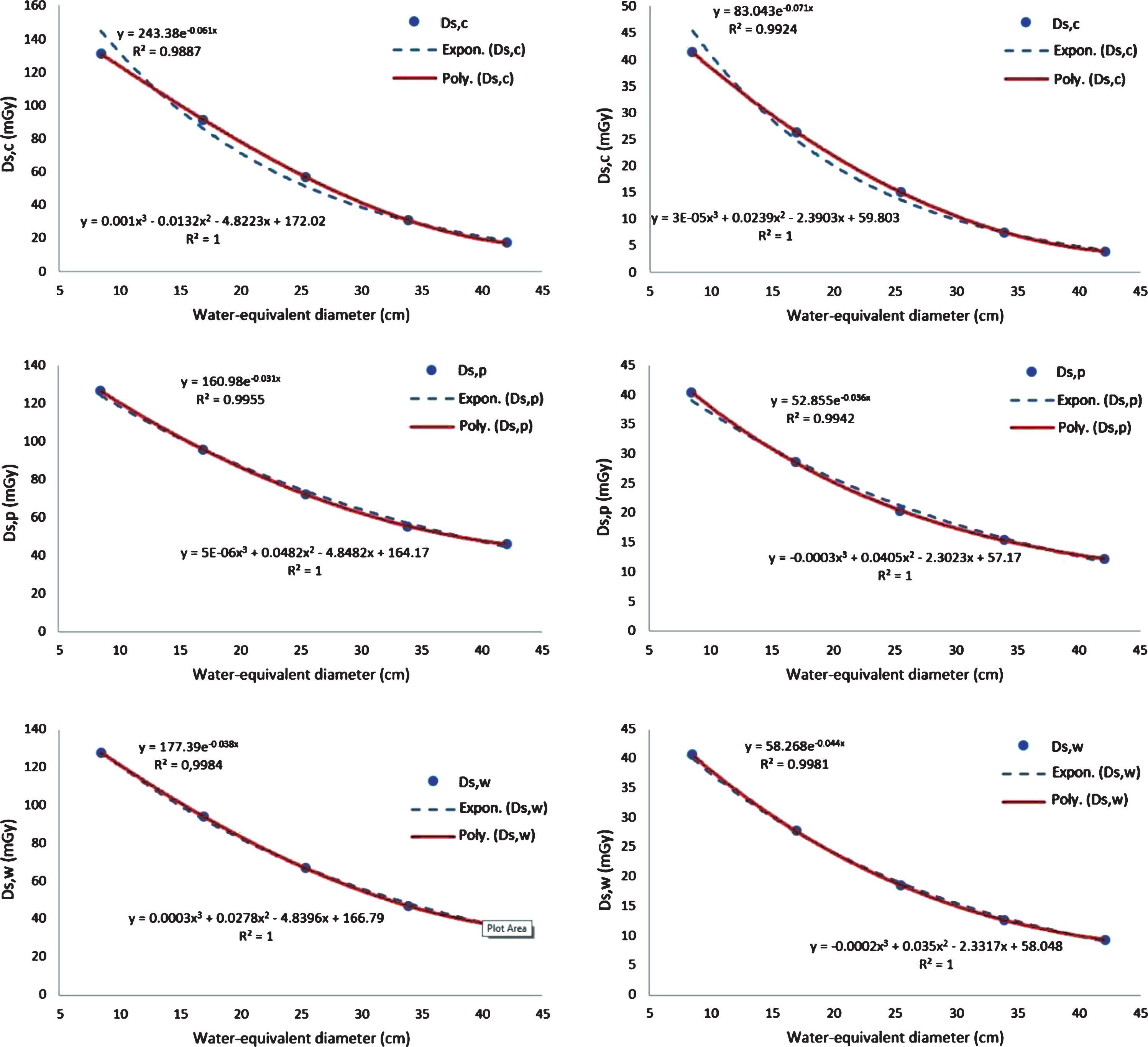
Size specific dose graphs for the water-equivalent diameter variation fitted by both exponential and third order polynomial regression, for tube voltages of 120 kVp and 80 kVp, are shown in Fig. 3. The results for tube voltages of 140 kVp and 100 kVp are not displayed, but they have a similar pattern to those in Fig. 3. The Ds,c, Ds,p, and Ds,w decrease with increasing water-equivalent diameter, as is already well-understood. The exponential regression is accurate for Ds,w, as reported previously [5, 34], however, Ds,c and Ds,p are more accurately fitted with a third order polynomial regression with a value of R2 = 1. Consequently, for the rest of the manuscript, exponential regression is used for Ds,w, while the third order polynomial regression is used for Ds,c and Ds,p.
Fig. 3
Size-specific dose (Ds) graphs for the water equivalent diameter variations. The Ds values are fitted with two types of regression, namely exponential and third order polynomial. The first row is for the Ds,c, the second row is for the Ds,p, and the third row is for the Ds,w. The first column is for a tube voltage of 120 kVp and the second column is for a tube voltage of 80 kVp.
3.2Ds,c, Ds,p, and Ds,w
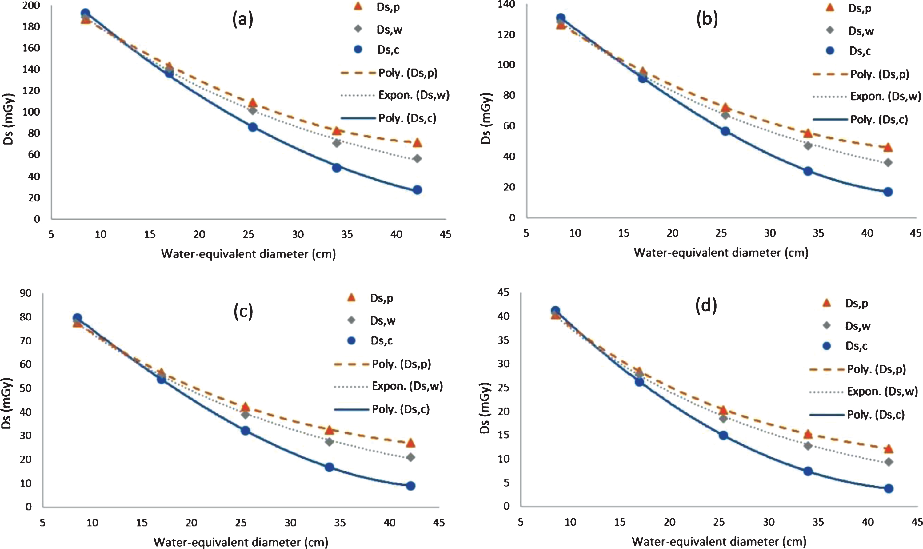
The graphs of Ds,c, Ds,p, and Ds,w for water-equivalent diameter variation at tube voltages from 80 kVp to 140 kVp are shown in Fig. 4. As the water-equivalent diameter increases, the Ds,c decreases fastest, followed by the Ds,w and then the Ds,p. The dose is not homogeneous between the centre and periphery of the phantom, which results in differences between the values of Ds,c and Ds,p. At large water-equivalent diameters, the Ds,p value is much greater than the Ds,c, while at small water-equivalent diameters, the Ds,p value is slightly smaller than Ds,c. However, at certain water-equivalent values (∼12–14 cm), the Ds values appear to be homogeneous, resulting in similar Ds,p and Ds,c values. The same pattern occurs in all the tube voltages from 80 kVp to 140 kVp.
Fig. 4
Comparisons of Ds,c, Ds,p, and Ds,w for various water-equivalent diameters (Dw), at tube voltages of (a) 140 kVp (b) 120 kVp (c) 100 kVp and (d) 80 kVp.
3.3Validation of weighted size-conversion factor (fw)
Before establishing the size-conversion factors for the central (fc) and peripheral (fp) phantom, the weighted size-conversion factors (fw) will be validated first. The fw for all tube voltages are normalized to the water-equivalent diameters of 33.90 cm (This value was chosen because it is the water-equivalent diameter value corresponding to the 32 cm physical diameter of the PMMA phantom [18]). All data are fitted with the exponential equation to create a single graph of the weighted size-conversion factor (Fig. 5a). To validate the result of this study, it is compared with the AAPM data [9] (Fig. 5b). It shows that the weighted size-conversion factors (fw) from this study are similar to the AAPM data with only small differences (i.e. within 5%).
Fig. 5
(a) The weighted size-conversion factors from all tube voltages fitted with the exponential equation. (b) Comparison of the weighted size-conversion factor data from this study with the AAPM data [9].
![(a) The weighted size-conversion factors from all tube voltages fitted with the exponential equation. (b) Comparison of the weighted size-conversion factor data from this study with the AAPM data [9].](https://content.iospress.com:443/media/xst/2020/28-4/xst-28-4-xst200667/xst-28-xst200667-g005.jpg)
3.4Size-conversion factors: fc, fp, and fw
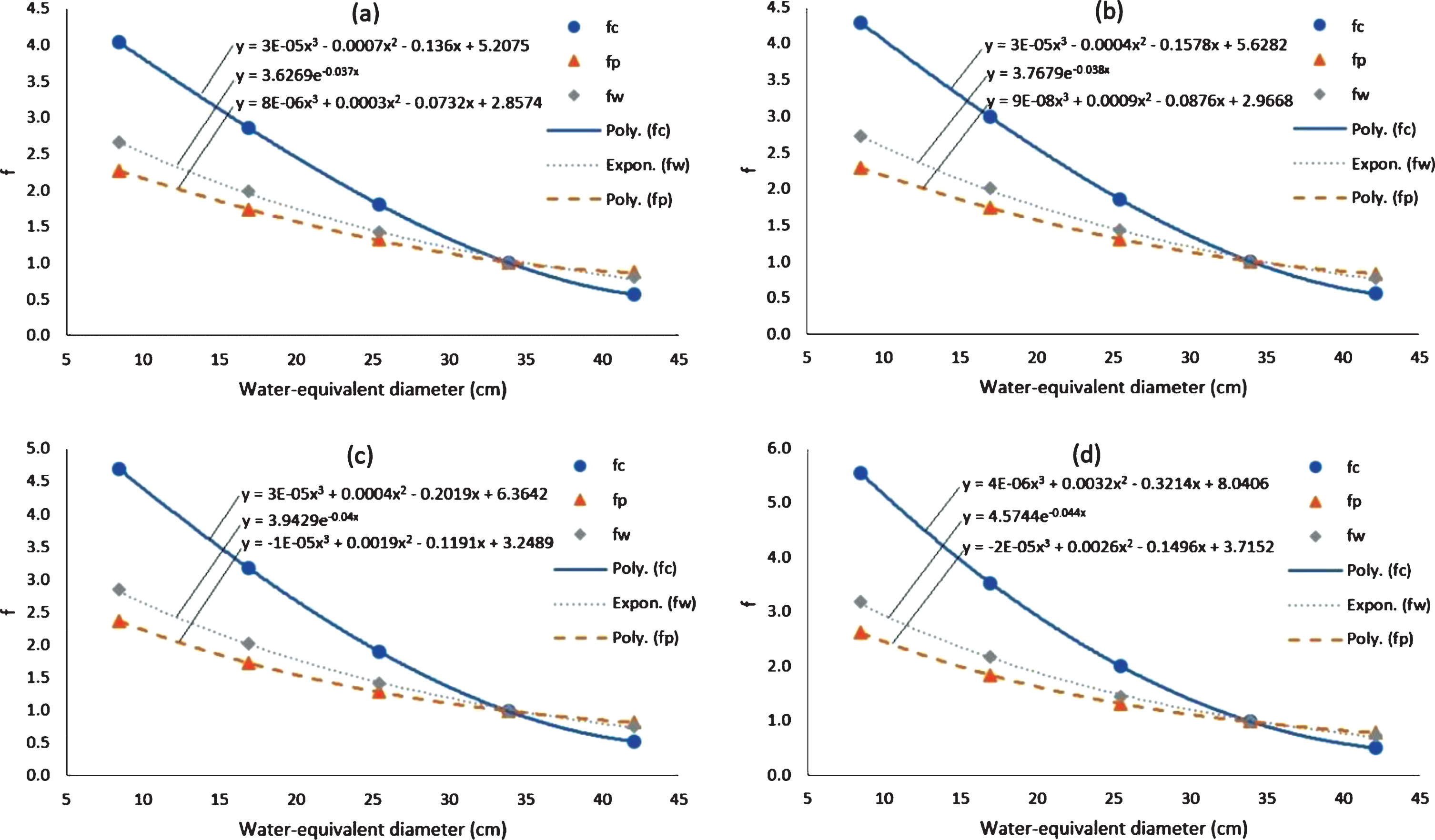
The size-conversion factors from CTDIvol to SSDE for the central (fc), peripheral (fp) and weighted centre-peripheral (fw) areas for various water-equivalent diameter at various tube voltages are shown in Fig. 6. Normalization is carried out at a water-equivalent diameter of 33.9 cm. The value of f decreases with increasing water-equivalent diameter. At small water-equivalent diameters, the fc value is much higher than fw, and the fp value is slightly smaller than fw. The same pattern is seen for four tube voltage variations from 80 kVp to 140 kVp. At small water-equivalent diameters, the values of fc, fp and fw are greater at small tube voltages (e.g. 80 kVp) than at large tube voltages (e.g. 140 kVp).
Fig. 6
Graphs of fc, fp, and fw for water-equivalent diameter variations at different tube voltages. Tube voltage of (a) 140 kVp, (b) 120 kVp, (c) 100 kVp, and (d) 80 kVp.
Hospital scientist and professional who are working in very busy environment, do not have enough time to extract conversion coefficients and dose values from graphs. Therefore, numerical values of fc, fp, and fw for water-equivalent diameter variations at different tube voltages are provided as a quick and convenient look up table in Table 1.
Table 1
Numerical values of fc, fp, and fw for water-equivalent diameter variations at different tube voltages
| Dw | fw | fc | fp | |||||||||
| (cm) | 140 kVp | 120 kVp | 100 kVp | 80 kVp | 140 kVp | 120 kVp | 100 kVp | 80 kVp | 140 kVp | 120 kVp | 100 kVp | 80 kVp |
| 8 | 2.70 | 2.78 | 2.86 | 3.22 | 4.09 | 4.35 | 4.79 | 5.68 | 2.29 | 2.32 | 2.42 | 2.68 |
| 9 | 2.60 | 2.68 | 2.75 | 3.08 | 3.95 | 4.20 | 4.60 | 5.41 | 2.23 | 2.25 | 2.33 | 2.57 |
| 10 | 2.51 | 2.58 | 2.64 | 2.95 | 3.81 | 4.04 | 4.41 | 5.15 | 2.16 | 2.18 | 2.24 | 2.47 |
| 11 | 2.41 | 2.48 | 2.54 | 2.82 | 3.67 | 3.88 | 4.22 | 4.90 | 2.10 | 2.11 | 2.16 | 2.37 |
| 12 | 2.33 | 2.39 | 2.44 | 2.70 | 3.53 | 3.73 | 4.04 | 4.65 | 2.03 | 2.04 | 2.08 | 2.27 |
| 13 | 2.24 | 2.30 | 2.34 | 2.58 | 3.39 | 3.57 | 3.86 | 4.42 | 1.97 | 1.98 | 2.01 | 2.18 |
| 14 | 2.16 | 2.21 | 2.25 | 2.47 | 3.25 | 3.42 | 3.68 | 4.18 | 1.91 | 1.91 | 1.93 | 2.09 |
| 15 | 2.08 | 2.13 | 2.16 | 2.36 | 3.11 | 3.27 | 3.51 | 3.96 | 1.85 | 1.85 | 1.86 | 2.01 |
| 16 | 2.01 | 2.05 | 2.08 | 2.26 | 2.98 | 3.12 | 3.34 | 3.74 | 1.79 | 1.79 | 1.80 | 1.92 |
| 17 | 1.93 | 1.97 | 2.00 | 2.17 | 2.84 | 2.97 | 3.17 | 3.53 | 1.73 | 1.73 | 1.73 | 1.85 |
| 18 | 1.86 | 1.90 | 1.92 | 2.07 | 2.71 | 2.83 | 3.01 | 3.32 | 1.68 | 1.67 | 1.67 | 1.77 |
| 19 | 1.80 | 1.83 | 1.84 | 1.98 | 2.58 | 2.69 | 2.84 | 3.12 | 1.62 | 1.62 | 1.61 | 1.70 |
| 20 | 1.73 | 1.76 | 1.77 | 1.90 | 2.45 | 2.55 | 2.69 | 2.93 | 1.57 | 1.56 | 1.55 | 1.64 |
| 21 | 1.67 | 1.70 | 1.70 | 1.82 | 2.32 | 2.41 | 2.54 | 2.75 | 1.52 | 1.51 | 1.50 | 1.57 |
| 22 | 1.61 | 1.63 | 1.64 | 1.74 | 2.20 | 2.28 | 2.39 | 2.57 | 1.47 | 1.46 | 1.45 | 1.51 |
| 23 | 1.55 | 1.57 | 1.57 | 1.66 | 2.08 | 2.15 | 2.24 | 2.40 | 1.42 | 1.41 | 1.40 | 1.46 |
| 24 | 1.49 | 1.51 | 1.51 | 1.59 | 1.96 | 2.03 | 2.10 | 2.24 | 1.37 | 1.37 | 1.35 | 1.40 |
| 25 | 1.44 | 1.46 | 1.45 | 1.52 | 1.85 | 1.90 | 1.97 | 2.08 | 1.33 | 1.32 | 1.31 | 1.35 |
| 26 | 1.39 | 1.40 | 1.39 | 1.46 | 1.74 | 1.78 | 1.84 | 1.93 | 1.28 | 1.28 | 1.27 | 1.30 |
| 27 | 1.34 | 1.35 | 1.34 | 1.39 | 1.63 | 1.67 | 1.71 | 1.79 | 1.24 | 1.24 | 1.23 | 1.26 |
| 28 | 1.29 | 1.30 | 1.29 | 1.33 | 1.53 | 1.56 | 1.59 | 1.65 | 1.20 | 1.20 | 1.19 | 1.21 |
| 29 | 1.24 | 1.25 | 1.24 | 1.28 | 1.43 | 1.45 | 1.48 | 1.53 | 1.16 | 1.16 | 1.15 | 1.17 |
| 30 | 1.20 | 1.21 | 1.19 | 1.22 | 1.33 | 1.35 | 1.37 | 1.41 | 1.13 | 1.13 | 1.12 | 1.13 |
| 31 | 1.15 | 1.16 | 1.14 | 1.17 | 1.24 | 1.25 | 1.26 | 1.29 | 1.09 | 1.09 | 1.09 | 1.09 |
| 32 | 1.11 | 1.12 | 1.10 | 1.12 | 1.15 | 1.16 | 1.17 | 1.19 | 1.06 | 1.06 | 1.06 | 1.06 |
| 33 | 1.07 | 1.08 | 1.05 | 1.07 | 1.07 | 1.08 | 1.07 | 1.09 | 1.03 | 1.03 | 1.03 | 1.02 |
| 34 | 1.03 | 1.04 | 1.01 | 1.02 | 0.99 | 0.99 | 0.99 | 0.99 | 1.00 | 1.00 | 1.00 | 0.99 |
| 35 | 0.99 | 1.00 | 0.97 | 0.98 | 0.92 | 0.92 | 0.91 | 0.91 | 0.98 | 0.97 | 0.97 | 0.96 |
| 36 | 0.96 | 0.96 | 0.93 | 0.94 | 0.85 | 0.85 | 0.84 | 0.83 | 0.96 | 0.95 | 0.95 | 0.94 |
| 37 | 0.92 | 0.92 | 0.90 | 0.90 | 0.79 | 0.78 | 0.77 | 0.76 | 0.93 | 0.92 | 0.93 | 0.91 |
| 38 | 0.89 | 0.89 | 0.86 | 0.86 | 0.73 | 0.73 | 0.71 | 0.70 | 0.92 | 0.90 | 0.90 | 0.88 |
| 39 | 0.86 | 0.86 | 0.83 | 0.82 | 0.68 | 0.67 | 0.66 | 0.64 | 0.90 | 0.88 | 0.88 | 0.86 |
| 40 | 0.83 | 0.82 | 0.80 | 0.79 | 0.64 | 0.63 | 0.61 | 0.60 | 0.89 | 0.86 | 0.87 | 0.84 |
| 41 | 0.80 | 0.79 | 0.76 | 0.75 | 0.60 | 0.59 | 0.57 | 0.55 | 0.88 | 0.85 | 0.85 | 0.82 |
| 42 | 0.77 | 0.76 | 0.73 | 0.72 | 0.57 | 0.56 | 0.54 | 0.52 | 0.87 | 0.83 | 0.83 | 0.80 |
3.5h-, k-, and p-factors
The h factor is the comparison between Ds,c and Ds,w, the k factor is the comparison between Ds,p and Ds,w, and the p factor is the comparison between Ds,p and Ds,c. The h-, k-, and p-factors for water-equivalent diameter variations at several tube voltages are shown in Fig. 7. At small water-equivalent diameters, the dose in the centre of the phantom (Ds,c) is slightly larger than at the periphery (Ds,p), but at large water-equivalent diameters, the dose in the centre of the phantom is much smaller than at the periphery of the phantom. These comparisons are also influenced by the tube voltage. At small tube voltages, the difference between the dose in the centre and the periphery is greater. Numerical values of h-, k-, and p-factors for water-equivalent diameter variations at different tube voltages are provided in Table 2.
Fig. 7
Graphs of the h-, k-, and p-factors plotted against the water equivalent diameters used for the four tube voltages, are shown in (a), (b) and (c) respectively.
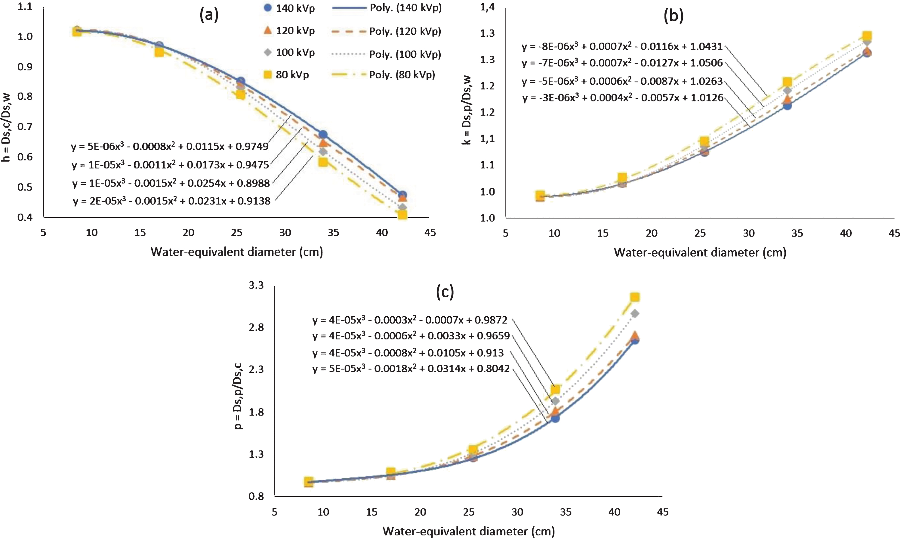
Table 2
Numerical values of the h-, k-, and p-factors for various water-equivalent diameters at different tube voltages
| Dw | h | k | p | |||||||||
| (cm) | 140 kVp | 120 kVp | 100 kVp | 80 kVp | 140 kVp | 120 kVp | 100 kVp | 80 kVp | 140 kVp | 120 kVp | 100 kVp | 80 kVp |
| 8 | 1.02 | 1.02 | 1.01 | 1.01 | 0.99 | 0.99 | 0.99 | 0.99 | 0.96 | 0.97 | 0.98 | 0.98 |
| 9 | 1.02 | 1.02 | 1.02 | 1.01 | 0.99 | 0.99 | 0.99 | 0.99 | 0.98 | 0.97 | 0.98 | 0.98 |
| 10 | 1.02 | 1.02 | 1.02 | 1.01 | 0.99 | 0.99 | 0.99 | 0.99 | 0.99 | 0.98 | 0.98 | 0.99 |
| 11 | 1.01 | 1.02 | 1.02 | 1.01 | 0.99 | 0.99 | 0.99 | 1.00 | 0.99 | 0.98 | 0.99 | 0.99 |
| 12 | 1.01 | 1.01 | 1.01 | 1.00 | 1.00 | 0.99 | 0.99 | 1.00 | 1.00 | 0.99 | 0.99 | 1.00 |
| 13 | 1.00 | 1.01 | 1.01 | 1.00 | 1.00 | 1.00 | 1.00 | 1.00 | 1.01 | 1.00 | 1.00 | 1.01 |
| 14 | 1.00 | 1.00 | 1.00 | 0.99 | 1.00 | 1.00 | 1.00 | 1.01 | 1.02 | 1.01 | 1.01 | 1.02 |
| 15 | 0.99 | 0.99 | 0.99 | 0.98 | 1.01 | 1.00 | 1.00 | 1.01 | 1.03 | 1.02 | 1.02 | 1.03 |
| 16 | 0.98 | 0.98 | 0.98 | 0.97 | 1.01 | 1.01 | 1.01 | 1.02 | 1.04 | 1.03 | 1.03 | 1.05 |
| 17 | 0.97 | 0.97 | 0.97 | 0.95 | 1.01 | 1.01 | 1.01 | 1.02 | 1.06 | 1.05 | 1.05 | 1.07 |
| 18 | 0.96 | 0.96 | 0.96 | 0.94 | 1.02 | 1.02 | 1.02 | 1.03 | 1.07 | 1.07 | 1.07 | 1.09 |
| 19 | 0.95 | 0.95 | 0.94 | 0.92 | 1.03 | 1.03 | 1.03 | 1.04 | 1.09 | 1.08 | 1.09 | 1.12 |
| 20 | 0.93 | 0.93 | 0.93 | 0.91 | 1.03 | 1.03 | 1.04 | 1.05 | 1.10 | 1.11 | 1.11 | 1.15 |
| 21 | 0.92 | 0.92 | 0.91 | 0.89 | 1.04 | 1.04 | 1.05 | 1.06 | 1.12 | 1.13 | 1.14 | 1.18 |
| 22 | 0.91 | 0.90 | 0.89 | 0.87 | 1.05 | 1.05 | 1.05 | 1.07 | 1.15 | 1.16 | 1.17 | 1.22 |
| 23 | 0.89 | 0.88 | 0.87 | 0.85 | 1.05 | 1.06 | 1.06 | 1.08 | 1.17 | 1.19 | 1.21 | 1.26 |
| 24 | 0.87 | 0.86 | 0.85 | 0.83 | 1.06 | 1.07 | 1.07 | 1.09 | 1.20 | 1.23 | 1.25 | 1.31 |
| 25 | 0.86 | 0.85 | 0.83 | 0.81 | 1.07 | 1.08 | 1.08 | 1.10 | 1.23 | 1.26 | 1.30 | 1.36 |
| 26 | 0.84 | 0.83 | 0.81 | 0.78 | 1.08 | 1.09 | 1.10 | 1.11 | 1.27 | 1.31 | 1.35 | 1.41 |
| 27 | 0.82 | 0.81 | 0.79 | 0.76 | 1.09 | 1.10 | 1.11 | 1.12 | 1.31 | 1.35 | 1.40 | 1.47 |
| 28 | 0.80 | 0.79 | 0.76 | 0.74 | 1.10 | 1.11 | 1.12 | 1.13 | 1.36 | 1.40 | 1.46 | 1.54 |
| 29 | 0.78 | 0.76 | 0.74 | 0.71 | 1.11 | 1.12 | 1.13 | 1.14 | 1.41 | 1.46 | 1.52 | 1.61 |
| 30 | 0.76 | 0.74 | 0.72 | 0.69 | 1.12 | 1.13 | 1.14 | 1.16 | 1.46 | 1.52 | 1.59 | 1.69 |
| 31 | 0.74 | 0.72 | 0.69 | 0.66 | 1.13 | 1.14 | 1.15 | 1.17 | 1.52 | 1.59 | 1.67 | 1.77 |
| 32 | 0.72 | 0.70 | 0.67 | 0.64 | 1.14 | 1.15 | 1.17 | 1.18 | 1.59 | 1.66 | 1.75 | 1.86 |
| 33 | 0.70 | 0.67 | 0.64 | 0.61 | 1.15 | 1.16 | 1.18 | 1.19 | 1.66 | 1.73 | 1.84 | 1.96 |
| 34 | 0.67 | 0.65 | 0.62 | 0.59 | 1.16 | 1.17 | 1.19 | 1.20 | 1.74 | 1.81 | 1.94 | 2.06 |
| 35 | 0.65 | 0.63 | 0.59 | 0.57 | 1.18 | 1.19 | 1.20 | 1.22 | 1.83 | 1.90 | 2.04 | 2.17 |
| 36 | 0.63 | 0.61 | 0.57 | 0.54 | 1.19 | 1.20 | 1.21 | 1.23 | 1.92 | 2.00 | 2.15 | 2.29 |
| 37 | 0.60 | 0.58 | 0.55 | 0.52 | 1.20 | 1.21 | 1.23 | 1.24 | 2.02 | 2.10 | 2.26 | 2.41 |
| 38 | 0.58 | 0.56 | 0.52 | 0.50 | 1.21 | 1.22 | 1.24 | 1.25 | 2.13 | 2.20 | 2.38 | 2.55 |
| 39 | 0.55 | 0.54 | 0.50 | 0.47 | 1.22 | 1.23 | 1.25 | 1.26 | 2.25 | 2.32 | 2.51 | 2.68 |
| 40 | 0.53 | 0.51 | 0.48 | 0.45 | 1.24 | 1.24 | 1.26 | 1.27 | 2.37 | 2.44 | 2.65 | 2.83 |
| 41 | 0.50 | 0.49 | 0.45 | 0.43 | 1.25 | 1.25 | 1.27 | 1.29 | 2.50 | 2.57 | 2.80 | 2.99 |
| 42 | 0.48 | 0.47 | 0.43 | 0.41 | 1.26 | 1.27 | 1.28 | 1.30 | 2.64 | 2.70 | 2.95 | 3.15 |
4Discussion
This study was carried out to determine the relationship between central, peripheral and weighted doses for variations in phantom sizes expressed in water-equivalent diameters. To the best of our knowledge, this study is the first to determine the dose distribution in phantoms of various diameters. Haba et al. [23] and Kim et al. [22], for example, have only investigated the dose distribution on the body and head phantoms. Haba et al. [23] reported that in a 32 cm phantom, the dose in the centre of the phantom is about 30% smaller than the dose at the periphery. Kim et al. [22], reported that the results of measuring the dose in the centre phantom is about 44% smaller than the dose at the periphery. For comparison, the current study found that in the physical phantom of 32 cm (Dw = 33.9 cm) that the dose at the centre of the phantom is around 42–52% smaller than at the periphery.
We found that in a small phantom (Dw < 12 cm), the dose is higher at the centre of the phantom than at the periphery. However, with an increase in phantom size, the dose distribution in the centre and peripheral areas changes. At a water-equivalent diameter of about 12–14 cm, the doses in the centre and peripheral areas are similar. For phantom sizes more than 14 cm, the dose at the centre is smaller than at the periphery, and the difference between both increases with further increases in phantom diameter. The larger sized phantoms cause a higher beam attenuation due to the longer path lengths of the beam, and these beams deposit less radiation at the centre compared to the periphery [22].
We also found that the dose ratio at the centre and at the periphery of the phantom was influenced by the magnitude of the tube voltage. The percentage difference between the central and peripheral doses increases with reduced tube voltages. This is due to a small voltage resulting in a smaller effective beam energy [35], and consequently the penetrating power is smaller and so the dose at the centre is small. As a result, the difference in the ratio of the dose at the centre and the periphery is large. The opposite results occur at large tube voltages.
This study obtained relationships between Ds,c, Ds,p, and Ds,w using the regression method. A previous study reported that the relationship between size-specific dose (Ds) and the water-equivalent diameter is described by exponential regression [34], and we have obtained the same result, but only for Ds,w. For Ds,c and Ds,p, a stronger (R2 = 1) relationship is found using a third order polynomial.
Based on the Ds,c, Ds,p, and Ds,w, the size-conversion factors at the centre (fc), periphery (fp), and weighted (fw) can be derived. The size-conversion factors are used to convert the CTDIvol to SSDE. Using these size conversion factors, we do not only obtain the weighted SSDE (SSDEw or simply stated as SSDE), but we also obtain the SSDEc and SSDEp. The SSDEc and the SSDEp can be obtained from the CTDIc and CTDIp values using the fc and fp conversion factors (Fig. 5). However, the only value displayed on the console and stored in the DICOM header is CTDIvol [36]. Therefore, determining the SSDEc and the SSDEp values from SSDEw (calculated the product of CTDIvol and fw) using the k and h factors as described in the Fig. 7 may be preferable.
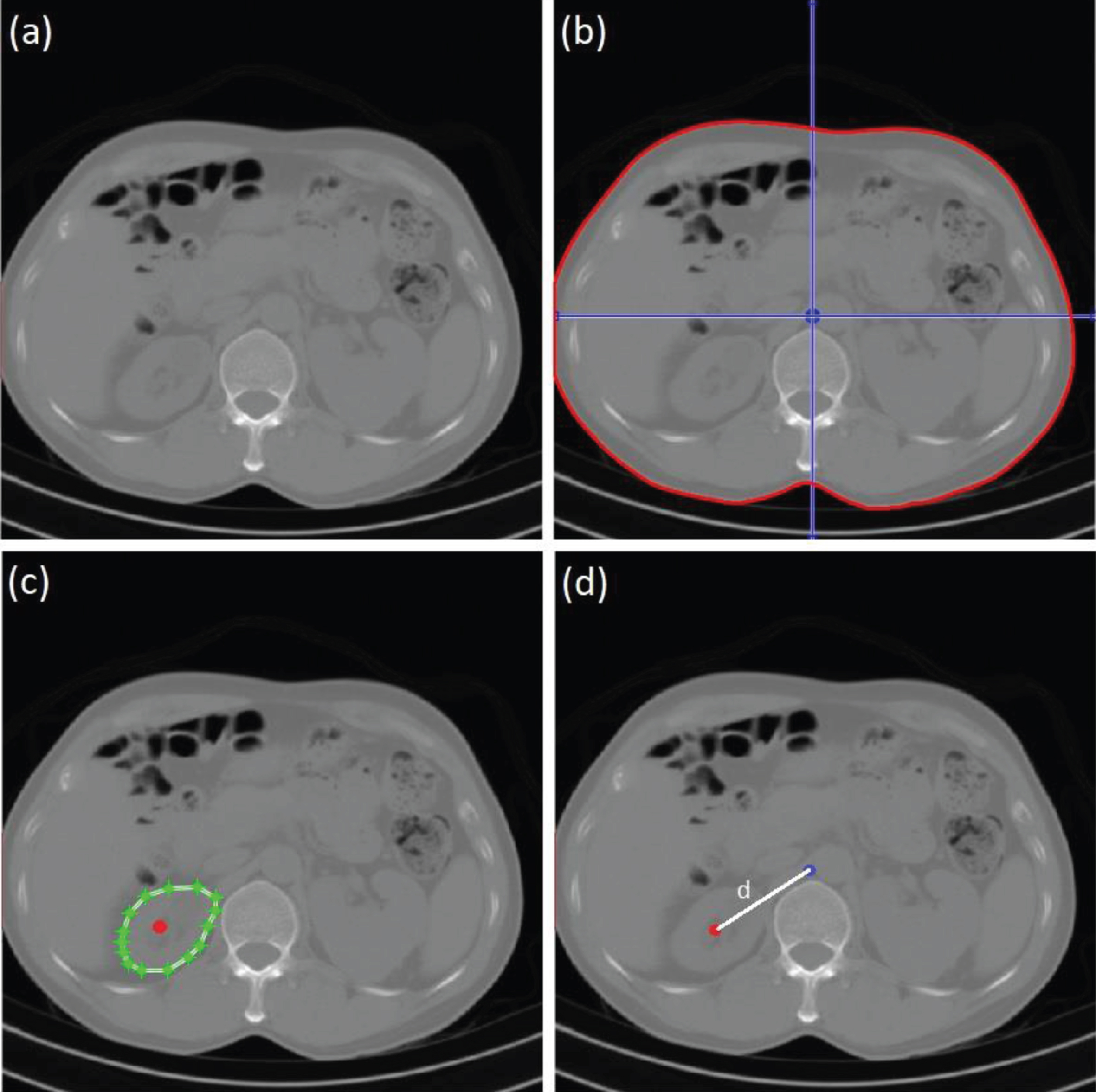
As mentioned in the introduction, the calculation of organ doses directly from the patient image is not yet an established methodology. Using the SSDEw value, the estimated organ dose, may have a relatively large uncertainty because the dose is not homogeneous throughout the patient as shown in Fig. 4. This is because the organs have notable variations in terms of position and volume. A more accurate dose estimation requires accurate information about the position and geometry of the organs [24, 31]. Direct organ doses may be obtained from patient images, by interpolation of SSDEc and SSDEp. Steps of estimating organ (e.g. left kidney) dose are as follows: First, the CTDIvol value is determined. It can be extracted from the DICOM header or from CT console. In this example, CTDIvol is 8.4 mGy. Because the pitch is 1, CTDw is similar to CTDIvol. Second, the water-equivalent diameter (Dw) [18] is then computed (In this example, the Dw is 25 cm) and the centre of the patient is determined (Fig. 8b). Third, fw is read from the Table 1. Because, the patient image is scanned using 120 kVp, the fw is 1.46. Fourth, the SSDEw value is then computed using Equation (14), and the result is 12.26 mGy. Fifth, the value of SSDEc and SSDEp can then be computed using Equations (16) and (17). The h and k factors are tabulated in Table 2, and in this example, h is 0.85 and k is 1.08, therefore the SSDEc is 10.42 mGy and SSDEp is 13.24 mGy. Sixth, the volume and the centre of the organ are determined (Fig. 8c). Seventh, distance (d) between the patient centre and organ centre is calculated. In this example, d is 6.0 cm (Fig. 8d). Lastly, the organ dose can be estimated by using linear interpolation between SSDEp and SSDEc, and the result of organ dose is approximately 11.83 mGy. This method can be computed rapidly using an automated method. It should be noted that this approach assumes that the dose is isotropically and radially distributed from the patient or phantom centre.
Fig. 8
Example images of organ (left kidney) dose estimation. (a) image of abdomen, (b) water-equivalent diameter and patient centre determination, (c) volume and organ centre determination, and (d) distance between centre of patient and centre of organ computation.
This methodology presents an opportunity to directly estimate the organ dose from the patient image. It represents an alternative method to determine organ doses in patients undergoing a CT scan. It is more straightforward than using either Monte Carlo simulations or measurements on physical phantoms. It may be more accurate in estimating organ doses for individual patients because the doses are directly calculated, which in turn can be used to more accurately predict cancer risk. However, the organ doses can only be calculated from the patient image if the organs are positioned in the scan area. Thus, conversion coefficients obtained in this study can be used with CTDIvol calculated based on 32 cm body phantom. Some abdominal examinations of children are based on 16 cm head phantom [37]. In these cases, the results of this study are not applicable.
5Conclusions
The distribution of doses in phantoms of various sizes have been investigated. It was found that the dose is relatively homogeneous for water-equivalent diameters between 12–14 cm. At a water equivalent diameter of less than 12 cm, the dose in the centre of the phantom is higher than at the periphery, and at water-equivalent diameters greater than 14 cm, the dose in the centre of the phantom is always less than at the peripheries. The difference in dose between the centre and the periphery is higher for larger water-equivalent diameters. It was also found that the dose distribution between the centre and the periphery is affected by the tube voltage used. At large water-equivalent diameter, the difference between central and peripheral doses is smaller for higher tube voltages. We found that the size-specific weighted dose (Ds,w) decreases exponentially with an increase in the water-equivalent diameter, but that the central (Ds,c) and peripheral doses (Ds,p) are better described by a third order polynomial.
Acknowledgments
This work was funded by the Riset Publikasi Internasional Bereputasi Tinggi (RPIBT) 2019, Universitas Diponegoro (Contract Number: 329-116/UN7.P4.3/PP/2019).
References
[1] | Perry B.J. and Bridges C. , Computerized transverse axial scanning (tomography): Part 3. Radiation dose considerations, Br J Radiol 46: ((1973) ), 1048–1051. |
[2] | Shope T.B. , Gagne R.M. and Johnson G.C. , A method for describing the doses delivered by transmission x-ray computed tomography, Med Phys 8: ((1981) ), 488–495. |
[3] | The Report of AAPM Task Group 204. Size-specific dose estimates (SSDE) in paediatric and adult body CT examinations, 2011. https://www.aapm.org/pubs/reports/RPT_204.pdf. |
[4] | Anam C. , Haryanto F. , Widita R. , et al., The evaluation of the effective diameter (Deff) calculation and its impact on the size-specific dose estimate (SSDE), Atom Indonesia 43: ((2017) ), 55–60. |
[5] | The Report of AAPM Task Group 220. Use of water equivalent diameter for calculating patient size and size-specific dose estimates (SSDE) in CT, 2014. https://www.aapm.org/pubs/reports/RPT_220.pdf. |
[6] | The Report of AAPM Task Group 293. Size-specific dose estimate (SSDE) for head CT, 2019. https://www.aapm.org/pubs/reports/RPT_293.pdf. |
[7] | Figueira C. , Di Maria S. , Baptista M. , et al., Paediatric CT exposures: comparison between CTDIVOL and SSDE methods using measurements and Monte Carlo simulations, Radiat Prot Dosim 165: ((2015) ), 210–215. |
[8] | Bashier E.H. and Suliman I.I. , Multi-slice CT examinations of adult patients at Sudanese hospitals: Radiation exposure based on size-specific dose estimates (SSDE), Radiol Med 123: ((2018) ), 424–431. |
[9] | Anam C. , et al., A simple method for calibrating pixel values of the CT localizer radiograph for calculating water-equivalent diameter and size-specific dose estimate, Radiat Prot Dosim 179: ((2018) ), 158–168. |
[10] | Yamazaki D. , et al., Usefulness of size-specific dose estimates in pediatric computed tomography: revalidation of large-scale pediatric CT dose survey data in Japan, Radiat Prot Dosim (2017), 1–9. doi:10.1093/rpd/ncx268 |
[11] | Kidoh M. , et al., Breast dose reduction for chest CT by modifying the scanning parameters based on the pre-scan size-specific dose estimate (SSDE), Eur Radiol 27: ((2017) ), 2267–2274. |
[12] | Larson D.B. , Optimizing CT radiation dose based on patient size and image quality: the size-specific dose estimate method, Pediatr Radiol 44: ((2014) ), S501–505. |
[13] | Anam C. , et al., Assessment of patient dose and noise level of clinical CT images: automated measurements, J Radiol Prot 39: ((2019) ), 783–793. |
[14] | Boos J. , et al., Institutional computed tomography diagnostic reference levels based on water-equivalent diameter and size-specific dose estimates, J Radiol Prot 38: ((2018) ), 536–548. |
[15] | Mohammadbeigi A. , et al., Local DRLs for paediatric CT examinations based on size-specific dose estimates in Kermanshah, Iran, Radiat Prot Dosim 186: ((2019) ), 496–506. |
[16] | Anam C. , Haryanto F. , Widita R. , et al., The size-specific dose estimate (SSDE) for truncated computed tomography images, Radiat Prot Dosim 175: ((2017) ), 313–320. |
[17] | Terashima M. , Mizonobe K. and Date H. , Determination of appropriate conversion factors for calculating size-specific dose estimates based on X-ray CT scout images after miscentering correction, Radiol Phys Technol 12: ((2019) ), 283–289. |
[18] | Anam C. , Haryanto F. , Widita R. , et al., Automated calculation of water-equivalent diameter (DW) based on AAPM task group 220, J Appl Clin Med Phys 17: ((2016) ), 320–333. |
[19] | Özsoykal I. , Yurt A. and Akgüngör K. , Size-specific dose estimates in chest, abdomen, and pelvis CT examinations of pediatric patients, Diagn Interv Radiol 24: ((2018) ), 243–248. |
[20] | Choudhary N. , Rana B.S. , Shukla A. , et al., Patients dose estimation in CT examinations using size specific dose estimates, Radiat Prot Dosim 184: ((2019) ), 256–262. |
[21] | Anam C. , Haryanto F. , Widita R. , et al., The impact of patient table on size-specific dose estimate (SSDE), Australas Phys Eng Sci Med 40: ((2017) ), 153–158. |
[22] | Kim S. , Yoshizumi T. , Toncheva G. , et al., Comparison of radiation doses between cone beam CT and multi detector CT: TLD measurements, Radiat Prot Dosim 132: ((2008) ), 339–345. |
[23] | Haba T. , Koyama S. and Ida Y. , Influence of difference in cross-sectional dose profile in a CTDI phantom on X-ray CT dose estimation: a Monte Carlo study, Radiol Phys Technol 7: ((2014) ), 133–140. |
[24] | Fujibuchi T. , et al., Estimate of organ radiation absorbed doses in clinical CT using the radiation treatment planning system, Radiat Prot Dosim 142: ((2010) ), 174–183. |
[25] | Sahbaee P. , Segars W.P. and Samei E. , Patient-based estimation of organ dose for a populationof 58 adult patients across 13 protocol categories, Med Phys 47: ((2014) ), 072104. |
[26] | DeMarco J.J. , et al., Estimating radiation doses from multidetector CT using Monte Carlo simulations: effects of different size voxelized patient models on magnitudes of organ and effective dose, Phys Med Biol 52: ((2007) ), 2583–2597. |
[27] | Tian X. , Li X. , Segars W.P. , et al., Pediatric chest and abdominopelvic CT: Organ dose estimation based on 42 patient models, Radiology 270: ((2014) ), 535–547. |
[28] | Najafzadeh M. , Nickfarjam A. , Jabbari K. , et al., Dosimetric verification of lung phantom calculated by collapsed cone convolution: A Monte Carlo and experimental evaluation, J Xray Sci Technol 27: ((2019) ), 161–175. |
[29] | Moore B.M. , Brady S.L. , Mirro A.E. , et al., Size-specific dose estimate (SSDE) provides a simple method to calculate organ dose for pediatric CT examinations, Med Phys 41: ((2014) ), 071917. |
[30] | Kalender W.A. , Dose in x-ray computed tomography, Phys Med Biol 59: ((2014) ), R129–150. |
[31] | Fearon T. , Xie H. , Cheng J.Y. , et al., Patient-specific CT dosimetry calculation: a feasibility study, J Appl Clin Med Phys 12: ((2011) ), 196–209. |
[32] | Adhianto D. , Anam C. , Sutanto H. , et al., The effect of phantom size and tube voltage on the size-conversion factor for patient dose estimation in CT examinations, Iran J Med Phys (2019). Doi: 10.22038/IJMP.2019.43059.1649 |
[33] | Kamezawa H. , Arimura H. , Arakawa H. , et al., Investigation of a practical patient dose index for assessment of patient organ dose from cone-beam computed tomography in radiation therapy using a Monte Carlo simulation, Radiat Prot Dosim 181: ((2018) ), 333–342. |
[34] | Abuhaimed A. , Martin C.J. and Demirkaya O. , Influence of cone beam CT (CBCT) scan parameters on size specific dose estimate (SSDE): A Monte Carlo study, Phys Med Biol 64: ((2019) ), 115002. |
[35] | Matsubara K. , Ichikawa K. , Murasaki Y. , et al., Accuracy of measuring half- and quarter-value layers and appropriate aperture width of a convenient method using a lead-covered case in X-ray computed tomography, J Appl Clin Med Phys 15: ((2014) ), 309–316. |
[36] | Anam C. , Haryanto F. , Widita R. , et al., A fully automated calculation of size-specific dose estimates (SSDE) in thoracic and head CT examinations, J Phys Conf Ser 694: ((2016) ), 012030. |
[37] | Shrimpton P.C. and Wall B.F. , Reference doses for paediatric computed tomography, Radiat Prot Dosimetry 90: ((2009) ), 249–252. |


