
Markov random field segmentation for industrial computed tomography with metal artefacts
Abstract
X-ray Computed Tomography (XCT) has become an important tool for industrial measurement and quality control through its ability to measure internal structures and volumetric defects. Segmentation of constituent materials in the volume acquired through XCT is one of the most critical factors that influence its robustness and repeatability. Highly attenuating materials such as steel can introduce artefacts in CT images that adversely affect the segmentation process, and results in large errors during quantification. This paper presents a Markov Random Field (MRF) segmentation method as a suitable approach for industrial samples with metal artefacts. The advantages of employing the MRF segmentation method are shown in comparison with Otsu thresholding on CT data from two industrial objects.
1Introduction
X-ray computed tomography (XCT) is a non-destructive visualization technique widely used in industrial metrology [1, 2], material composition and micro-structure studies [3, 4], and medical analysis [5]. XCT is advantageous over other measurement techniques such as coordinate measuring machine (CMM) and optical scanning because it can capture volumetric data that is not accessible using other methods. XCT allows measurement of internal and external geometries of industrial components as well as quantification of volumetric defects. Intermetallic phases and voids in alloys can be studied for understanding metallurgical procedures and improving alloy composition [3].
XCT is based on the principle of attenuation of X-rays as they pass through an object, where the attenuation depends upon the material they interact with and energy of the X-rays. The received intensity of X-rays at the detector result in a 2D projection, with numerous projections taken through a full rotation of the object. A 3D CT volume is then generated by reconstructing these projections by methods such as filtered back-projection [6]. This volume is a map of linear attenuation coefficients. Segmentation of different constituent materials can then be extracted from the CT volume based on the measured attenuation of groups of voxels (3D pixels) resulting in several distinct labels. Following segmentation, dimensional and material analysis can be performed on the volume.
There are several influence factors that affect XCT performance such as: scanning parameters, part dimension, orientation and geometry, and CT system hardware geometry and performance [2, 7–10]. Robustness and repeatability of XCT analysis particularly depends on the segmentation strategy, making it a critical step in the process [11]. However, image artefacts can severely impact segmentation and lead to uncertainty in quantification [12, 13]. A particular issue with high material densities is beam hardening [14] where there is a preferential attenuation of lower energy X-rays. This results in cupping artefacts where a homogeneous object appears to have grey values that are higher at the periphery of the object boundary. Resulting from the part geometry and orientation, X-rays passing through varying lengths of the material in a single projection can lead to non-uniform grey values in the reconstructed images. In this case, a skewed material phase in the grey value histogram of the CT volume is observed. As these histograms are the basis of global image segmentation, a clear separation between the imaged materials is degraded.
Image noise is another common issue where associated grey values are not homogenous for a single material (or background). Some level of noise naturally occurs in lab-based XCT due to the polychromatic beam where X-rays produced are not of a single energy and therefore have different levels of attenuation. The reconstruction methods assume a monochromatic beam, which it is not, causing the introduction of noise into the CT volume. Further hardware variations such as detector intensity variations between projections also contribute to this noise. In fact, a detector pixel could exhibit a continuous distinct variation from its neighbours throughout all projections. In this case, the reconstruction smears this pixel through the CT volume resulting in ring artefacts. Scanning parameters that result in a low amount of received photons either through low intensity of X-rays received by the detector, fast image acquisition, or a fewer number of projections to reconstruct similarly influence the noise level in the CT volume [6].
While absorption is the primary attenuation in XCT, there is also a degree of scatter which is particularly evident when scanning high density objects. Scatter results in localized grey value variations in the CT volume represented as noise, streaks, shades, bands and blurred boundaries [15]. In medical studies, similar issues are encountered when scanning metal implants due to the presence of streaks and shades. To improve qualitative interpretation of these images, several metal artefact reduction (MAR) algorithms [16–18] have been developed, providing the radiologist with a clearer representation of the data. However, they can generate secondary artefacts by fixing the distortions and lead to misrepresentation in areas close to metal objects [19, 20]. It must be noted that these techniques may not be useful in quantitative industrial applications [21] where introducing secondary artefacts and misrepresentations could lead to inaccurate measurement.
ISO-50 and Otsu [22] are widely used segmentation techniques in XCT as advised in the British Standard BS 16016 [23] and various best practice guides such as that by National Physics Laboratory [24]. These methods are reliant on the calculation of a global threshold value to classify pixels. Their prevalent use in industrial XCT is evident across numerous published works as they work well with low noise data and have been shown to give accurate results in industrial contexts, particularly in dimensional measurement [1, 2, 4, 11, 25].
There are alternative more complex segmentation methods that have shown promise in the more general field of XCT but have yet to be given appreciation in published standards and usage guides. Watershed segmentation [4, 26] that is frequently used in multi-material segmentations uses an initial seeding for materials together with gradient information from the image to classify pixels through constrained region growing. Multi-material segmentations are particularly problematic in common industrial objects where there are metallic and rubber/plastic phases. One way to overcome this is by using a combination of region growing and graph-cut methods as demonstrated in [27]. There are of course many more for consideration that also have merit over standard global thresholding as in Otsu and ISO50. This is of particular importance where XCT volumes have local grey value variations, streaks, bands and other imaging artefacts that lead to questionable segmentations and therefore inaccurate results.
In light of this discussion, alternative approaches to segmentation for industrial XCT require consideration, particularly in the presence of numerous imaging artefacts. Modelling using a Markov Random Field (MRF) to segment regions or detect edges may be helpful in such cases. It is expected that nearby pixels in a region have same or similar labels, representing some global context. Given the contextual information, a label assigned to a pixel should not only depend upon its grey value but also on the labels of its neighbouring pixels; spatial information like region smoothness is lost in techniques like Otsu, whereas Markov Random Fields incorporate both local knowledge and global context [28, 29]. MRFs and have been used in the analysis of medical images [30] and in the development of MRF based MAR algorithms [31].
This article focuses on improved segmentation of CT images in the case of scatter, streaks, loss of contrast, and noisy data using MRFs. First, the MRF image segmentation method is outlined. Otsu and MRF are then applied to two test objects demonstrating high levels of noise, non-uniformities, streaks and banding. When evaluating the appropriateness of methodologies in X-ray CT scanning or segmentation, it is normative to consider a calibrated sample of known dimensions [2, 25] or porosity [32]. In this way, the true measure is known and provides a direct comparison on the accuracy of the method. This paper uses real samples that produces unique banding, streaking and non-uniformities in the CT volume that would be difficult to replicate in a calibrated sample. In this manner, a qualitative comparison is made that highlights advantages and limitations of both methods and suggestions on usage are given when applied to such difficult cases.
2Method
2.1Markov random field image segmentation
Let S ={ s1, …, sn } be a set of sites (pixels) in an image, and let Λ = { 1, . . . , M} be the set of possible labels (background, material etc.) that can be assigned to the sites for a multi-level logistic model [33]. An assumption is made which states that pixel values corresponding to each label λ ∈ Λin the image follow a Gaussian distribution with θλ ={ μλ, σλ } . F = { F1, … , Fn } a collection of random variables is a random field on S in which each Fi takes a value fi in the label set Λ. The joint event F = f denotes Fi = fi∀ i ∈ { 1, …, n }. The probability of this joint event is p (f) where f ={ f1, … , fn } is a configuration of F. The random field F an be regarded as a random variable taking its values in the set of all possible labellings or configuration space ΛS = Λ * Λ * … * Λ, n times. A neighbourhood system N is defined for an MRF which relates sites to one another. The local property of MRFs states that a variable is conditionally independent of all other variables given its neighbours. Context-dependent entities are implemented in MRFs by virtue of the local property through this neighbourhood system. From the set of all possible labellings ΛS, the objective is to find a labelling
(1)
From Bayes’ theorem, the conditional probability of labelling configuration f given observed data d can be expressed as
(2)
(3)
(4)
For a labelling f over all sites S,
(5)
The joint likelihood probability can be written as:
(6)
(7)
From equations (5) & (7), energy can be derived as
(8)
Where K is a constant. The joint likelihood energy for a labelling f is
(9)
The likelihood energy represents the likelihood of sites belonging to a label with the assignment favouring the label for which energy is minimum. The distribution characteristics θΛ = {μ1, μ2, …, μM, σ1, σ2, …, σM} are crucial to the definition of likelihood function and are estimated using Maximum Likelihood.
The prior conveys the contextual information in a region or overall image. To derive the prior energy, a neighbourhood system is defined and cliques are identified. Cliques are subsets of sites in image space such that every pair of sites in a clique are neighbours. The labellings of sites in a clique determine clique potentials from a predefined potential function Vc The energy of the Gibbs distribution can be expressed as a summation of clique potentials for the defined neighbourhood system [35]:
(10)
By specifying the potential functions, the prior distribution for the MRF is defined. Consider a 2nd order neighbourhood system N in an image region shown in Fig. 1.
Fig.1
A second order neighbourhood in an image region.
Only single-site and pair-site cliques are considered for this discussion. Neighbours of site x are given by N (x) ={ 1, 2, 3, 4, 5, 6, 7, 8 } The cliques which are a superset of site x are:
1. single-site x, and
2. pair-sites x - 1, x - 2,..., x - 8
Appropriate clique potentials can be built for specific applications. Clique potentials for single-site cliques can be given by
(11)
Clique potentials for pair-sites can be given by a constant, a bounded quadratic or other functions along with weight or interaction parameter, β such that cliques which have different label elements have higher potential than those with similar elements. In the case of a smoothing prior, similar neighbouring sites are given an incentive by a negative potential and differing sites a penalty by a positive potential:
(12)
A pair-site clique has a negative potential β when labels of constituent sites are the same and a positive potential -β when labels of constituent sites are different. The parameters φ ={ α1, …, αM, β } can be estimated using least squares fitting [35] on an overdetermined system of linear equations derived from distinct configurations of neighbouring labels. Since clique potentials are now defined, the prior distribution of the MRF is defined. The posterior probability can be expressed in terms of posterior energy and thus, a MAP estimate can be expressed in terms of likelihood and prior energies:
(13)
(14)
Minimizing the posterior energy U (f|d) is too computationally expensive due to a large search space. Thus, an iterative local maximization technique called Iterated Conditional Modes (ICM) [28] is used that maximizes conditional probabilities of sites sequentially. In other words, it iteratively minimizes the posterior energy of each site given all other sites, U (fi|d, fS-{i}). Initialization of the algorithm is usually done with labels obtained by minimizing the likelihood energy for each site. Since we are working with many XCT slices, we employ a stability tracking algorithm [36] to enable ICM to converge faster by avoiding unnecessary evaluations. After initial assignments, a site label may change if and only if labels of any of its neighbours change. This is a direct conclusion of the local Markov property. Posterior energies for possible labels of a site will only be evaluated if any of its neighbours updated their label in the previous iteration. Using ICM it is feasible to introduce problem dependent constraints to achieve better segmentations.
2.2Test strategy
In order to assess the performance of MRF and Otsu, objects of different materials, geometries and characteristic defects were scanned.
2.2.1Steel column
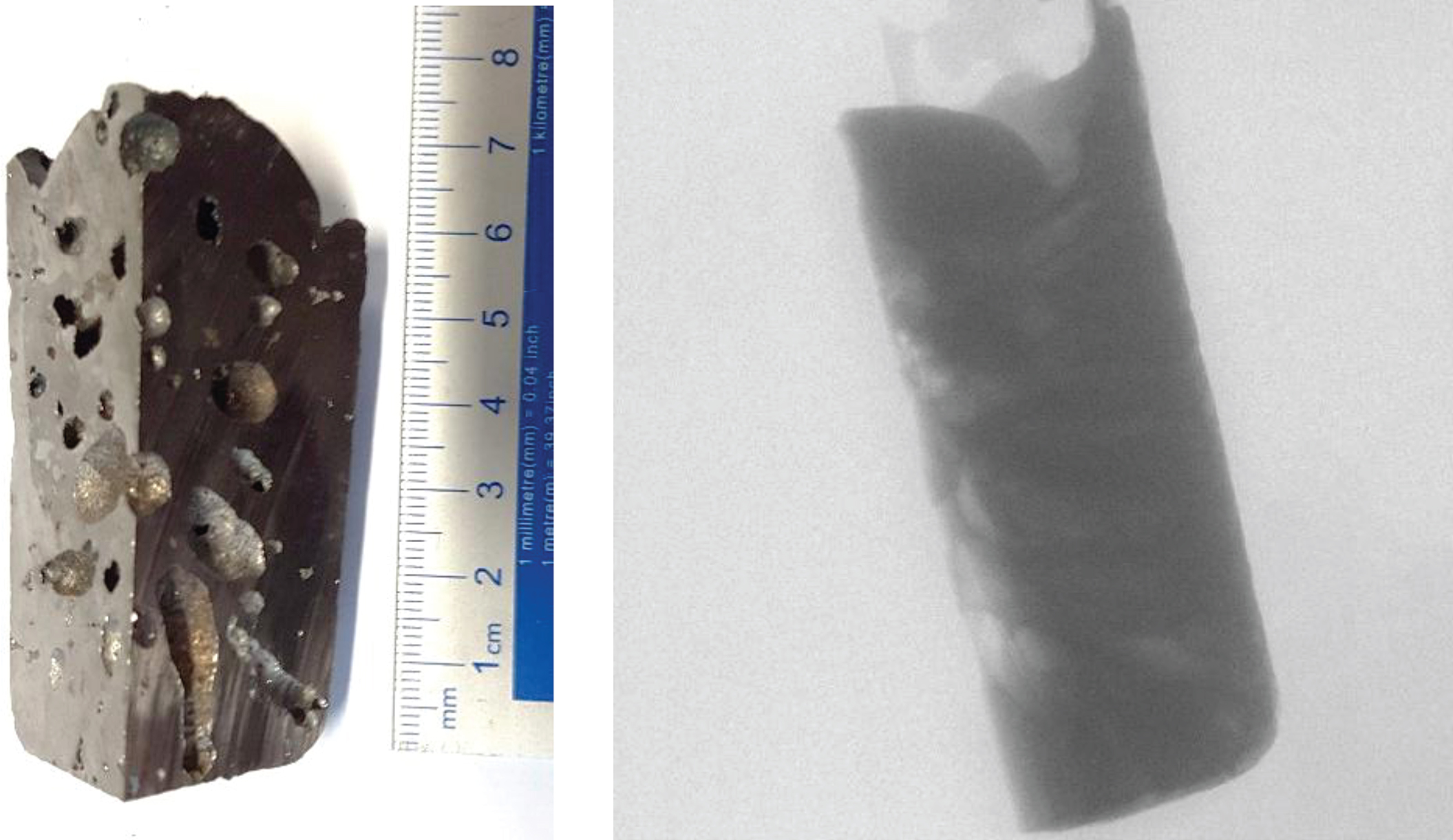
The first object is a steel column pictured in Fig. 2 of quarter circle cross section measuring approximately 80 mm in height and a radius of 36 mm. It is a part of a mold of steel taken from a basic oxygen furnace and divided into four to allow shorter path lengths for X-rays to achieve sufficient penetration. The sample has several voids of different sizes and shapes due to the production of carbon monoxide that often gets trapped in the steel. The segmentation of these voids serves as a metric in the experiments. Studying porosity of samples manufactured with different process parameters is of interest to materials engineers to determine optimal manufacture. The high iron content makes it a difficult object to image at a higher resolution as it requires high energy and intensity X-rays to penetrate which give rise to significant scatter and beam hardening artefacts. In addition, the geometry of the sample has some sharp corners that under any scanning orientation can lead to inhomogeneity in grey values due to large variations in path lengths traversed by the X-ray beam in that region.
Fig.2
Steel column workpiece and representative radiograph that is used throughout the analysis.
2.2.2Titanium cuboid
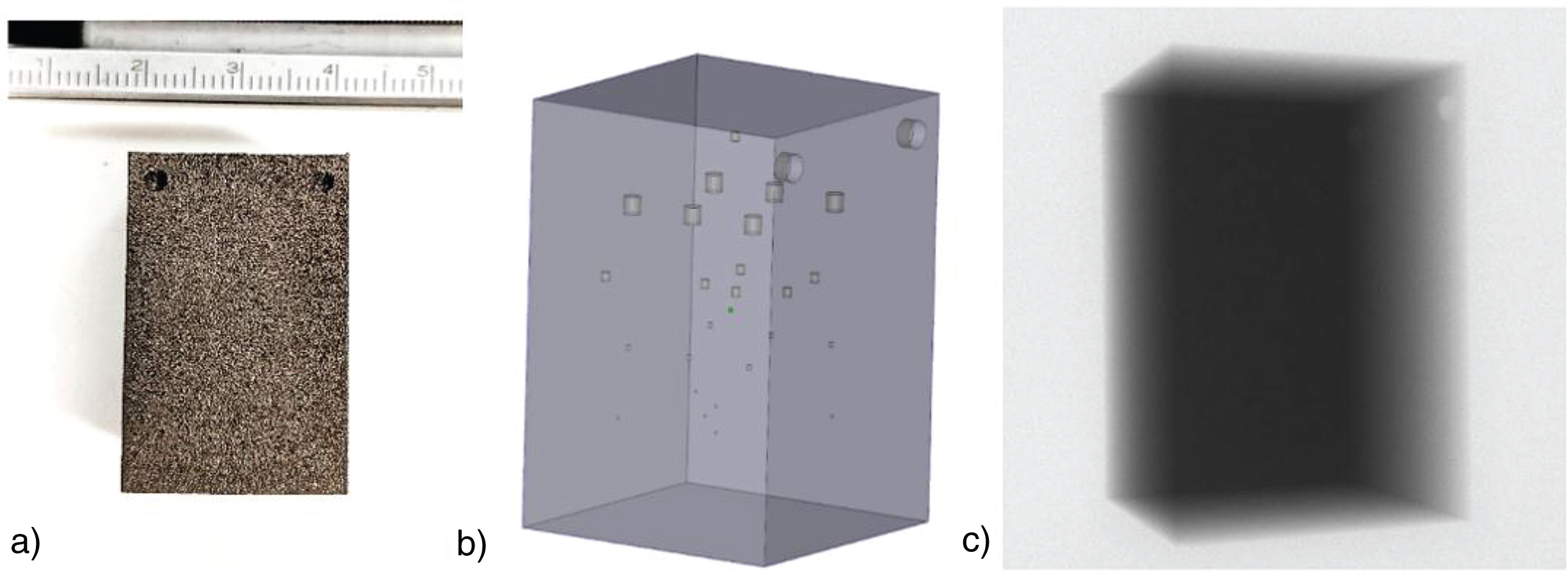
The second object is an additively manufactured cuboid of Ti6Al4V measuring 30 mm in height with a square cross section of side 20 mm. The sample has a number of prescribed cylindrical voids varying from 0.2–1.2 mm in diameter as shown in the CAD model in Fig. 3 b), in this case used to study the efficacy of the segmentation. Given its metallic composition, again the reconstructed volume will exhibit scattering radiation artefacts particularly around sharp edges and interior voids.
Fig.3
a) Titanium cuboid workpiece, b) CAD of object showing placement of voids and c) representative radiograph.
3Experiments
3.1Experimental procedure
The samples were scanned in a Nikon XT H 225/320 LC XCT scanner using parameters shown in Table 1. The machine has a fixed source and detector with a manipulator to position and rotate the sample, taking 2D projections at numerous angular intervals. The projections show visually the attenuation of X-rays traversing the sample where individual pixels have an associated value referred to as the grey value due to their representation.
Table 1
XCT scanning parameters for the samples
| Parameter | Steel column | Titanium cuboid |
| Voltage (kV) | 310 | 215 |
| Current (μA) | 97 | 433 |
| Filter (mm Sn) | 6 | 5 |
| Exposure (s) | 4 | 0.5 |
| # projections | 3141 | 3141 |
| Detector pixel size (μm) | 200 | |
| Voxel size (μm) | 38 | 19 |
| CT volume size x (y z voxels) | 2000×2000×2000 | |
| Scan time (min) | 210 | 27 |
The projections were reconstructed using filtered back-projection [6] within Nikon proprietary software that results in a stack of 2D slices through the object. Together they provide a volumetric representation of the sample with 3D pixels or voxels that have an associated grey value equivalent to the absorptivity of the material at that point. A beam hardening reduction filter was applied in the reconstruction process to remove residual cupping imaging artefacts. The filter used was a standard polynomial correction (second order) where the function attempts to transform the polychromatic attenuation data into equivalent monochromatic data, often referred to as linearisation [37].
After reconstruction, the samples were segmented using Otsu thresholding and the MRF method outlined in Section 2.1 in order to compare the advantages and disadvantages of their application. The built-in greythresh() function in MATLAB (Image Processing and Parallel Computing Toolboxes Release 2016b, The MathWorks, Inc., Natick, Massachusetts, United States) was used for Otsu thresholding. The discussed MRF method and its least squares parameter estimation were coded as a MATLAB script.
3.2CT scan data
CT images obtained from scanning the two objects are presented and their characteristic artefacts are discussed. The grey values lie in the range [0, 1] for all the CT images presented in this article.
3.2.1Steel column
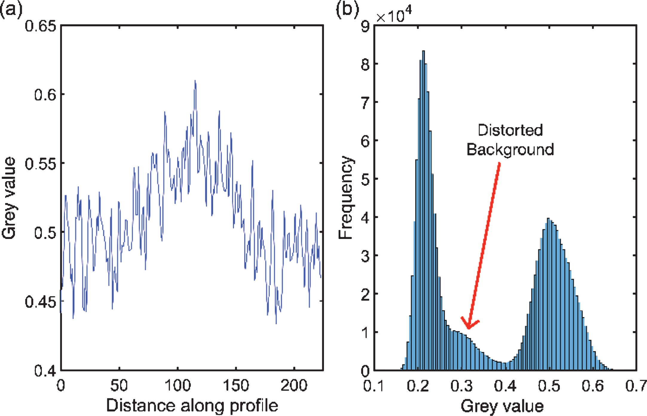
Slices acquired from the steel column exhibit streaks, loss of contrast, and noise as shown in Fig. 4(a). Different artefacts and specific features are marked with arrows and white rectangles respectively in Fig. 4(b). Voids suffer from loss of contrast and inhomogeneous grey values due to high scatter and are marked with white arrows. Smaller voids which have been obscured due to scatter are indicated with blue arrows. Scatter and beam hardening cause beam attenuation to become non-linear to path-length, causing non-uniform grey values in the CT image. Yellow arrows indicate streaks emanating from high contrast regions such as voids resulting in inhomogeneity in grey values in homogenous regions. This inhomogeneity can be observed in the line profile across a streak in Fig. 5(a). The image grey value histogram shown in Fig. 5(b) shows the absence of a sharp valley between background and material due to high amounts of scatter contributing to non-uniform nature of background grey values. Segmentation results of voids highlighted by white rectangles in Fig. 4(b) are shown in Fig. 10 and discussed in section 4.1.
Fig.4
(a) An image from XCT scan of the steel column. (b) Arrows and rectangles show different artefacts and features respectively, see text for details.
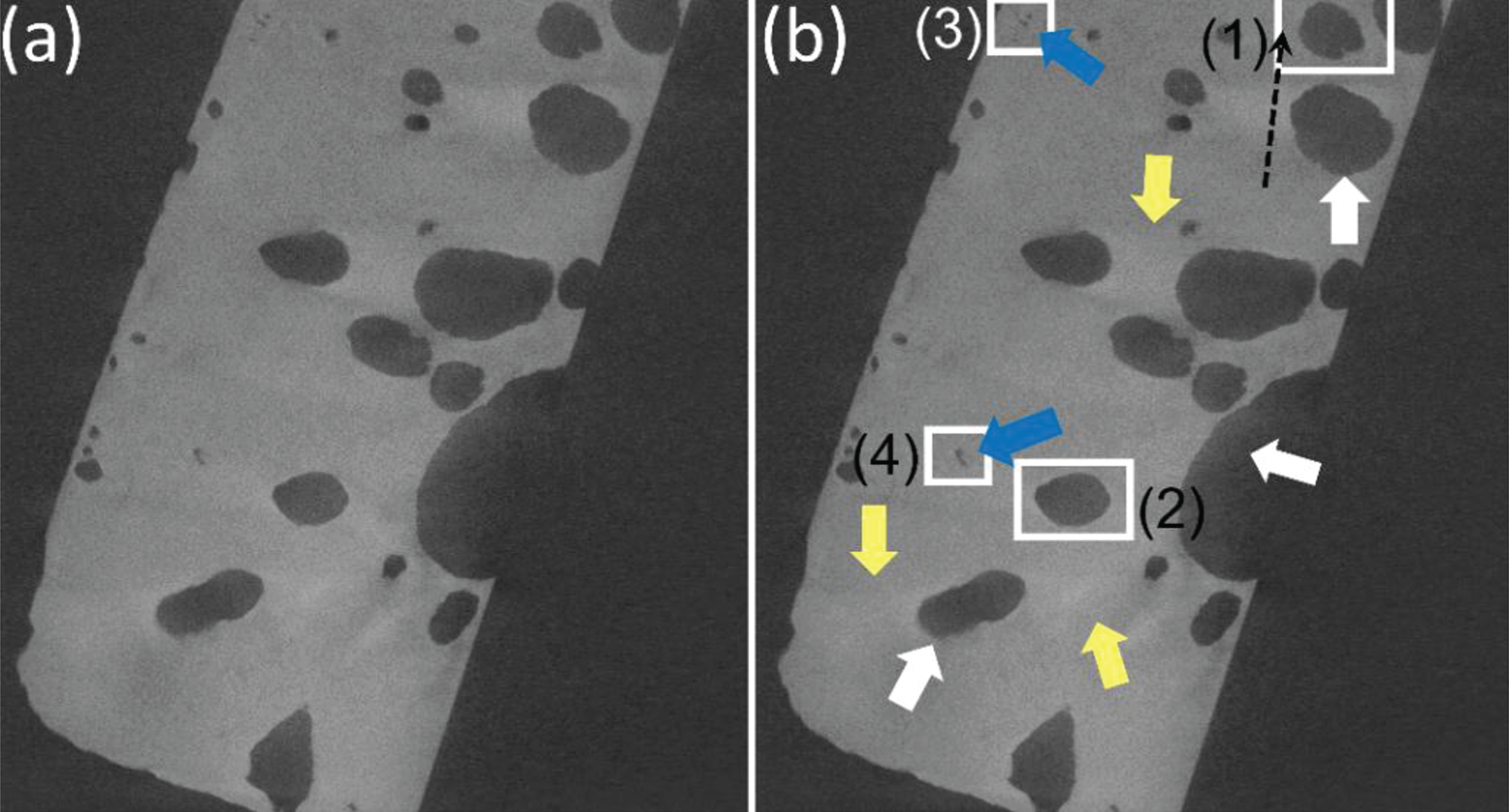
Fig.5
(a) Line profile along the black dashed arrow shown in Fig. 3(b), and (b) histogram for CT image in Fig. 3(a).
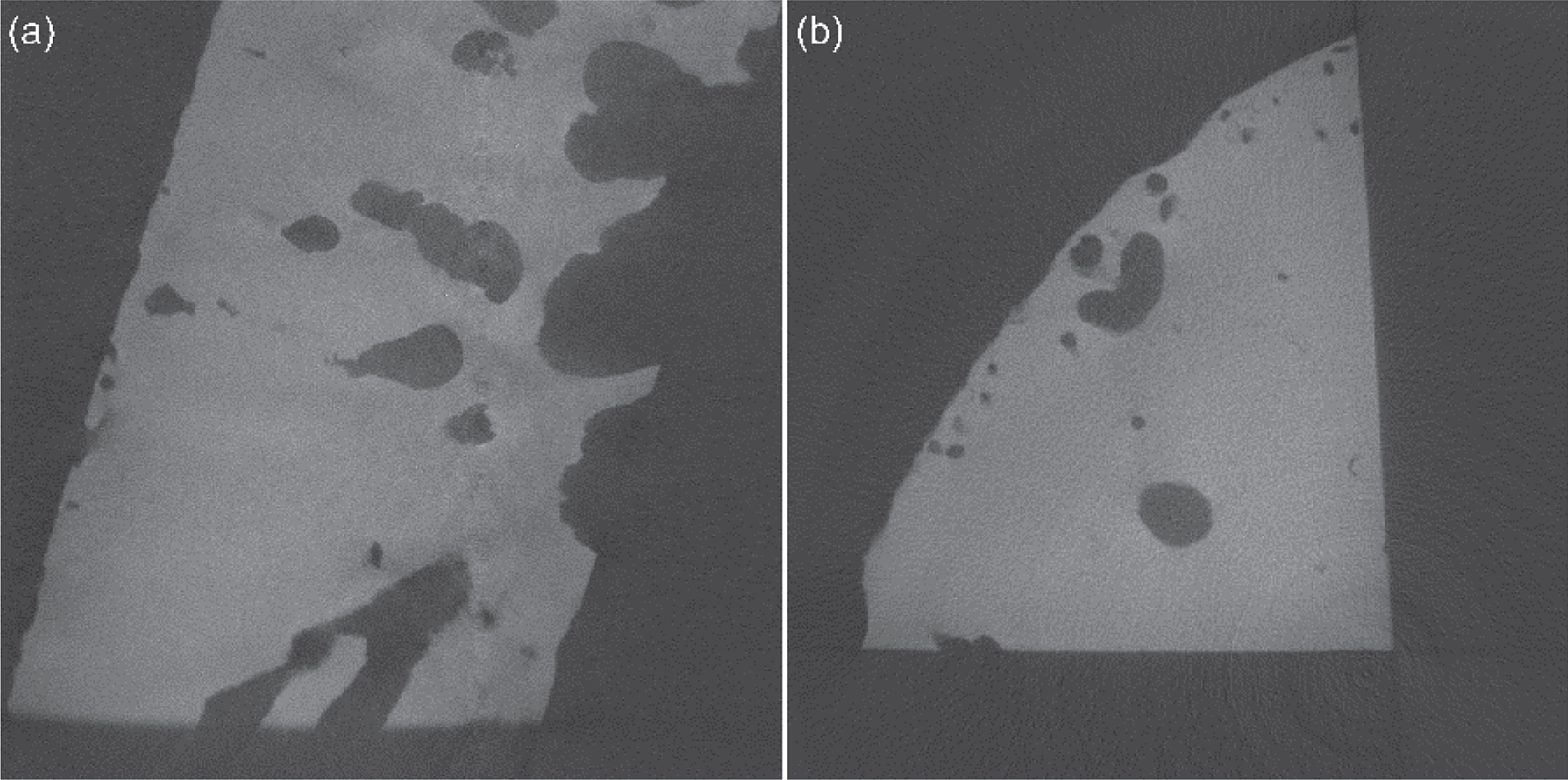
To study the effect of part geometry on artefacts and subsequent segmentation, CT slices are considered in two orthogonal directions. Figure 6 shows two more CT images of the steel column. Image (a) shows a cross-section closer to the object boundary having edges and voids severely affected by scatter and ring artefacts with their axis parallel to the image plane. Image (b) has several small voids where the ability to successfully segment across the two methods is of particular interest.
Fig.6
CT images (a) of the same orientation, and (b) orthogonal to image in Fig. 3(a). Note that (b) is smaller and has less material than (a) and has been cropped and resized for visualization.
3.2.2Titanium cuboid
One of the XCT images of titanium cuboid is shown in Fig. 7(a). It shows streaks emanating from sharp corners, and loss of contrast indicated by yellow arrows, and white arrows respectively in Fig. 7(b). The black dashed line in Fig. 7(b) is used to generate the line profile in Fig. 8. The holes within the cuboid suffer from loss of contrast due to scatter similar to obscured voids in the steel column. Non-linearity between attenuation and path length causes a cupping artifact, showing the interior of the object to be less attenuating than it is. This further promotes loss of contrast experienced by the holes. Table 2 shows means and standard deviations of rectangular sections marked 1–4, in Fig. 7(b).
Fig.7
(a) A CT image of the titanium cuboid, and (b) same image with arrows showing artefacts and rectangles indicating areas of interest. See text for details.
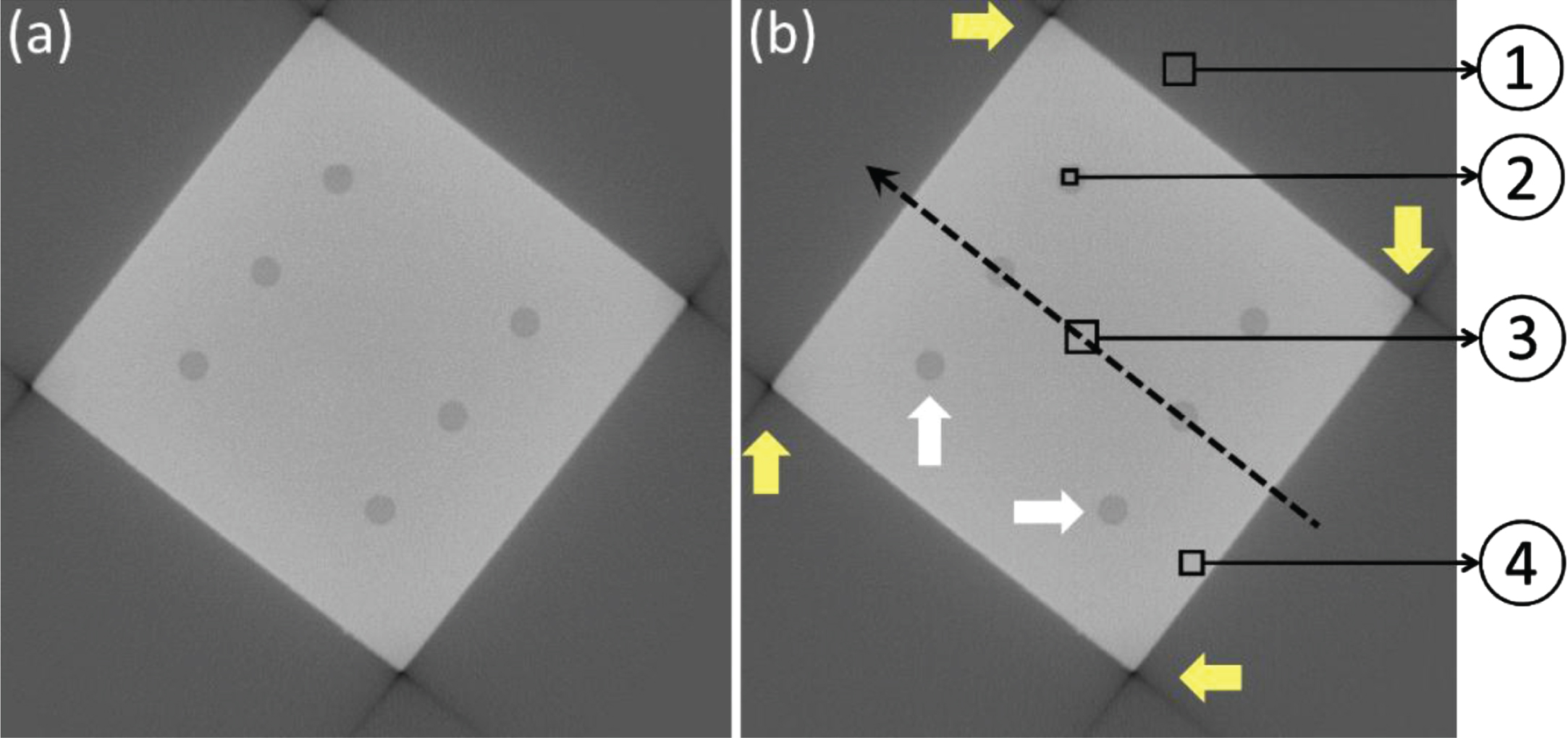
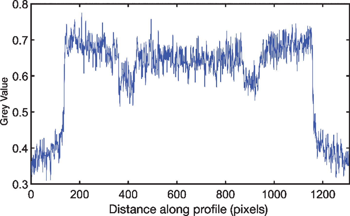
Table 2
Means, standard deviations and true labels for the rectangular sections from Fig. 6(b). True label shows the correct classes of these regions
| Region (refer Fig. 7(b)) | Mean grey value | Standard deviation | True region (material/background) |
| 1 | 0.3809 | 0.0247 | External Background |
| 2 | 0.5771 | 0.0301 | Void Background |
| 3 | 0.6407 | 0.0309 | Inner Material |
| 4 | 0.6900 | 0.0263 | External Material |
Figure 8 and Table 2 demonstrate loss of contrast in the holes and cupping artefact in the image. It is observed that regions 1 and 2 which are both background have quite different grey values due to high scatter. This can lead to incorrect segmentation.
4Results and discussion
MRF segmentation and Otsu methods were applied to the resultant scans from the steel column and titanium cuboid. When testing new segmentation methods it is common to use computer designed images where the ground truth is known. MRFs have previously been demonstrated as a successful segmentation tool in this manner [22, 38]. Here, MRF segmentation’s capabilities and limitations are explored using real lab-produced data.
4.1Steel column
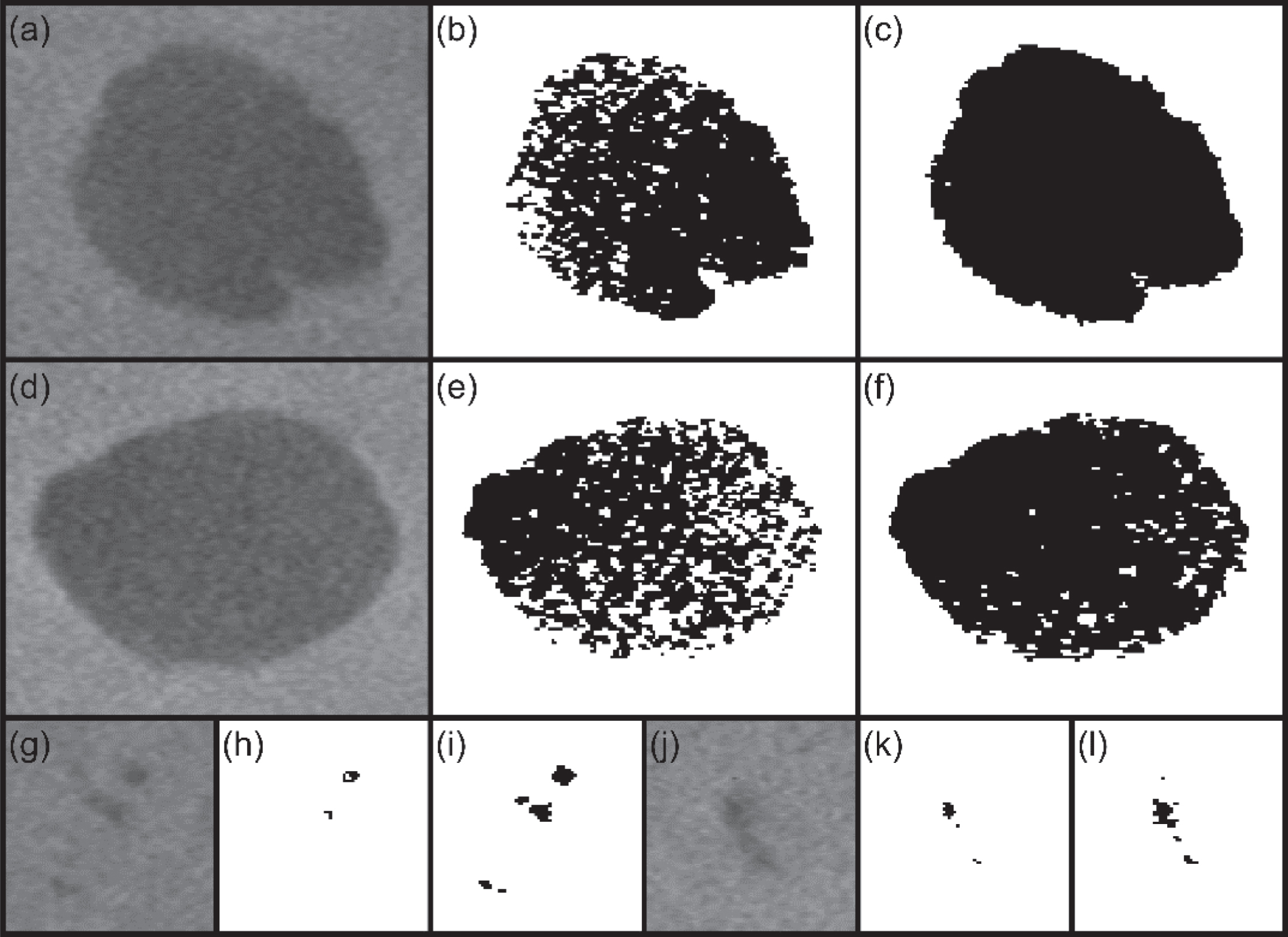
Loss of contrast severely affects Otsu’s performance to classify voids correctly as can be observed in Fig. 9. Upon visual inspection, it is clear that a large number of background pixels are identified as material and smooth edges are scarcely seen. The MRF method classifies such voids correctly. Figure 10 shows segmentation results of four voids shown inside rectangles in Fig. 3(b). Voids (1) and (2) show improvement when MRF segmentation is used. Voids (3) and (4) being small and easily concealed by scatter, are not successfully segmented by Otsu whereas the MRF method appears to resolve them with greater accuracy.
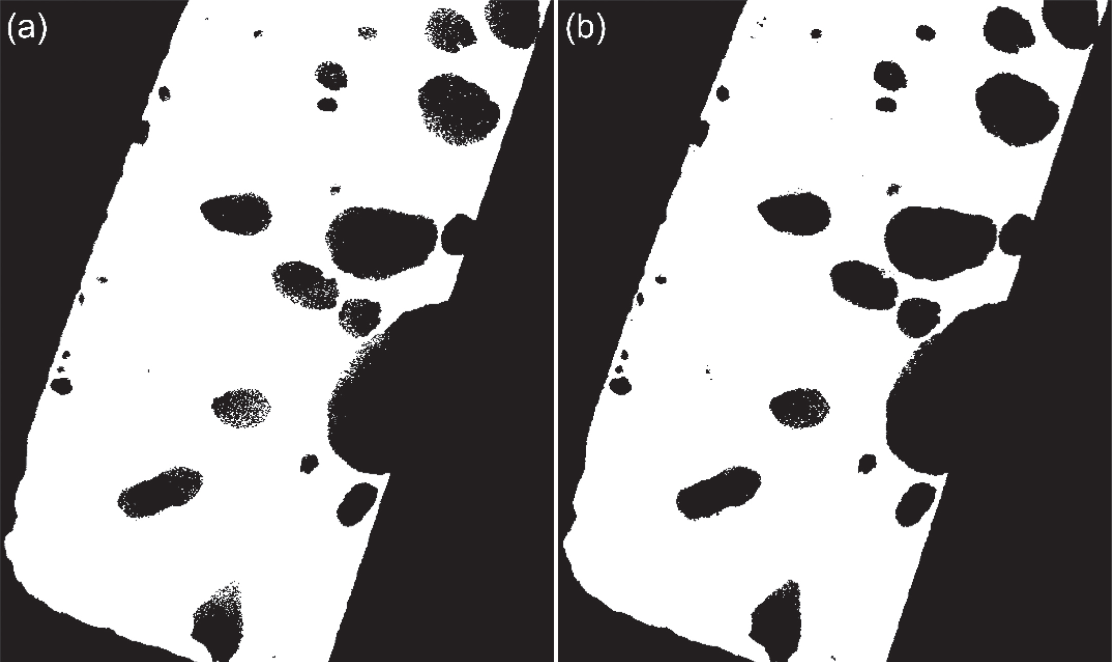
Fig.10
Several voids in the steel column (a), (d), (g) and (j) marked in Fig. 3(b) as (1), (2), (3) and (4) along with their Otsu (b), (e), (h) and (k), and MRF segmentations (c), (f), (i) and (l) respectively.
ICM for the MRF method was initialized by likelihood energy minimization for each pixel in the image. It takes ICM an average of 6 iterations to converge to local minima for all images in the stack. The number of evaluations of posterior energy is kept at a minimum at each iteration using stability tracking. Table 3 summarizes ICM’s average performance over 1400 images in steel column CT stack.
Table 3
ICM performance for the steel column CT stack. Note that the calculations do not include border pixels of the image. Posterior for border pixels is not evaluated because of unavailability of 8-point neighbourhoods; they assume the label assigned to them in ICM initialization
| Iteration | % pixels evaluated | % pixel labels changed | Number of changes per evaluation |
| 1 | 100.00 | 0.1417 | 0.0014 |
| 2 | 0.5329 | 0.0174 | 0.0326 |
| 3 | 0.0736 | 0.0036 | 0.0491 |
| 4 | 0.0155 | 0.0009 | 0.0577 |
| 5 | 0.0039 | 0.0002 | 0.0624 |
| 6 | 0.0011 | 0.0001 | 0.0662 |
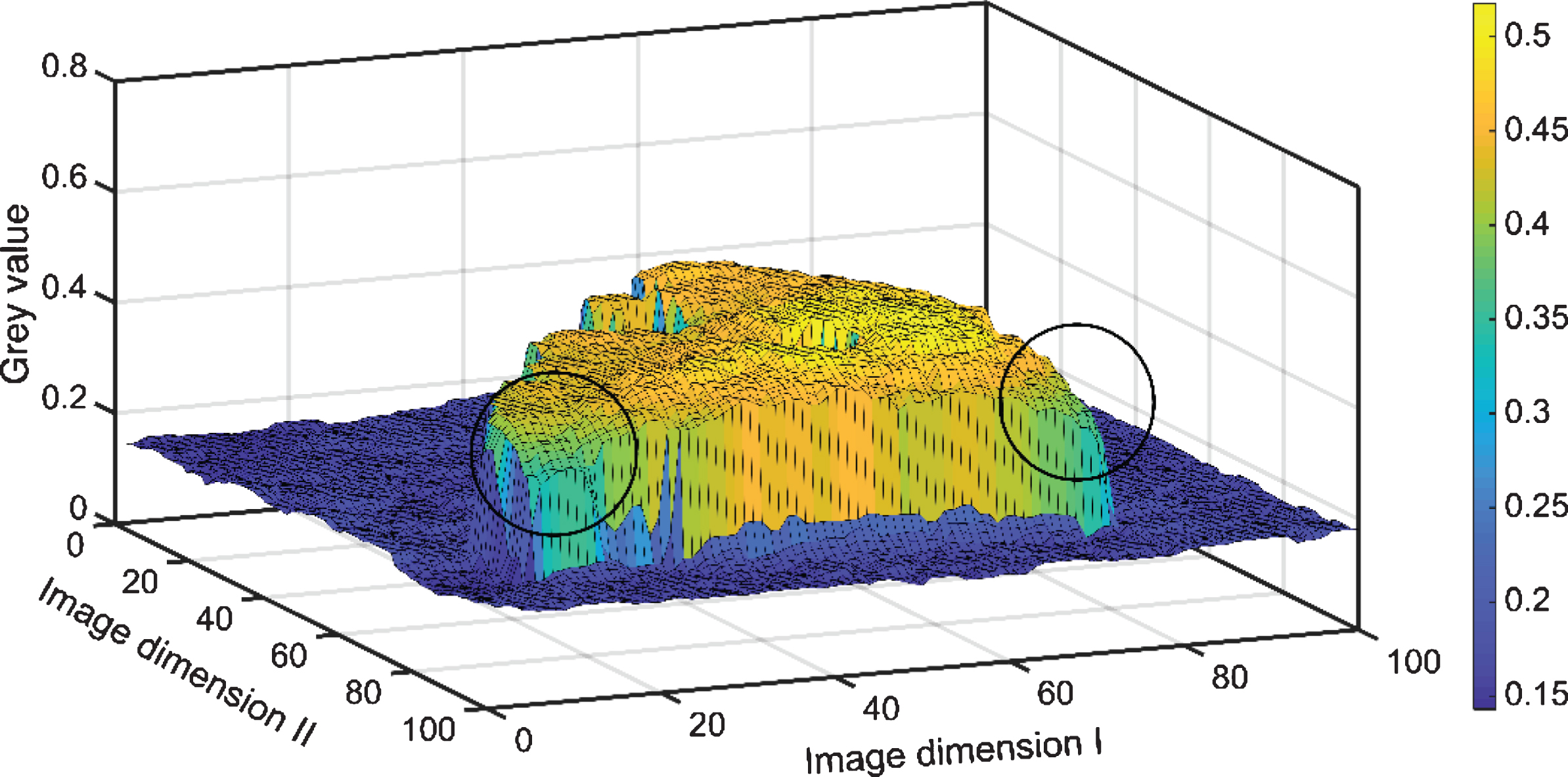
Comparison between Otsu and MRF results shown in Fig. 11 validates that in the case of scatter affecting voids, improved segmentation is possible using MRF. But it is observed that the corners of the steel column are degraded in MRF’s output more than Otsu. Investigating this effect further, it can be seen from the grey value surface plot in Fig. 12 that corners have lower grey values than rest of the material. This inhomogeneity is a result of the geometry of the object and the non-linear relation of attenuation with path-length compounded as non-uniform grey value distribution.
In the MRF segmentation, the label assigned to a pixel may change if the change in prior energy which is based on neighbours, overcomes the change in likelihood (global) energy during posterior energy minimization. Therefore, corner pixels with lower grey values having background neighbours might be labelled background themselves as ICM progresses.
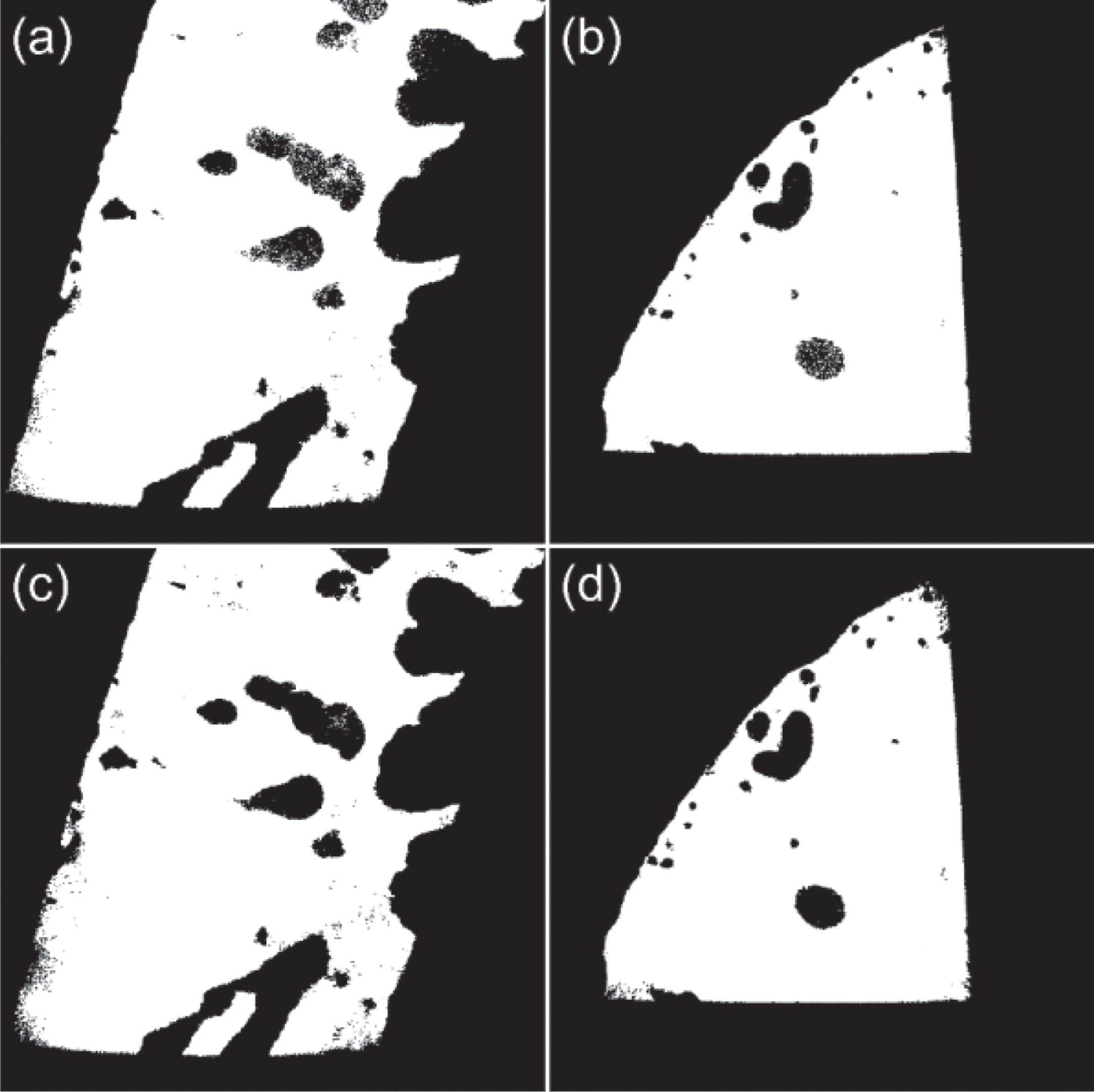
Fig.12
The CT image in Fig. 6(b) plotted as a surface. The two lower corners are highlighted where there are issues with grey values appearing lower than normal.
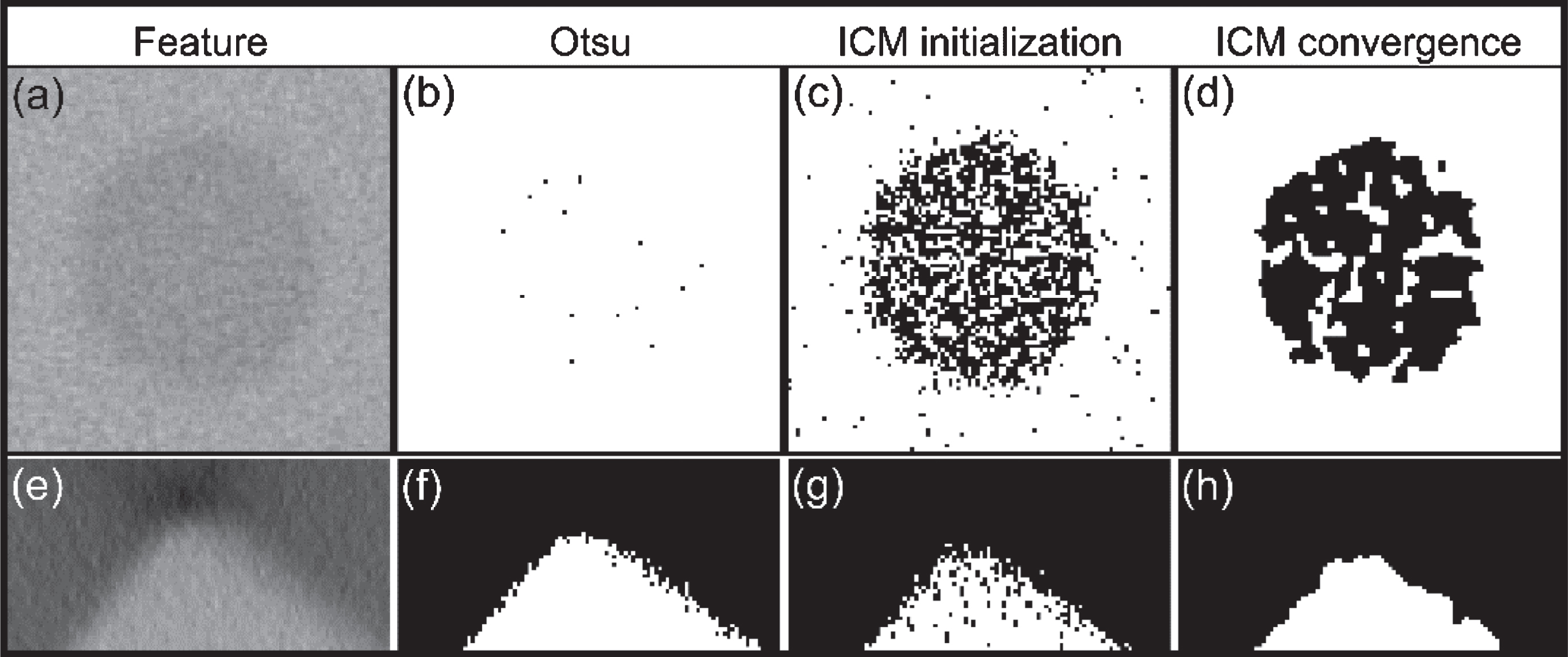
Consider the CT image in Fig. 13(a) to demonstrate how geometry and poor contrast can influence segmentation. The grey value distribution in Fig. 13(b) shows that the image is affected by a loss of contrast and the presence of background ‘fringes’ in the material is observed. The segmentation results for Otsu, ICM initialization label field, and ICM convergence are compared in Fig. 14. It is observed that the corner is poorly segmented by both Otsu and MRF suggesting that it is the scan itself that is problematic rather than the segmentation method.
Fig.13
(a) A CT image from steel column showing corner and voids with poor contrast, and (b) its grey value distribution highlighted by a red/blue colour transform.
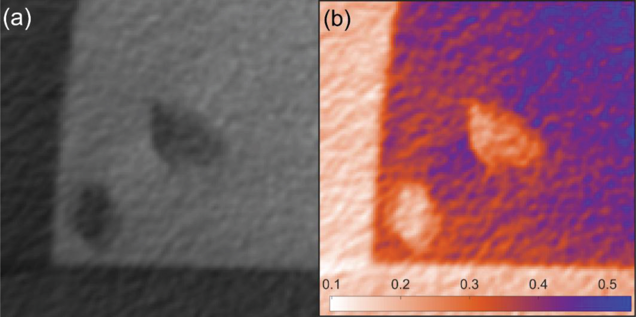
Fig.14
(a) Otsu result, (b) ICM initialization, (c) ICM converges for CT image shown in Fig. 12(a). Error in each case is evaluated as a percentage of incorrectly labelled material pixels in all material pixels. Note that both Otsu and MRF were applied on the whole image and a cropped section is shown here.
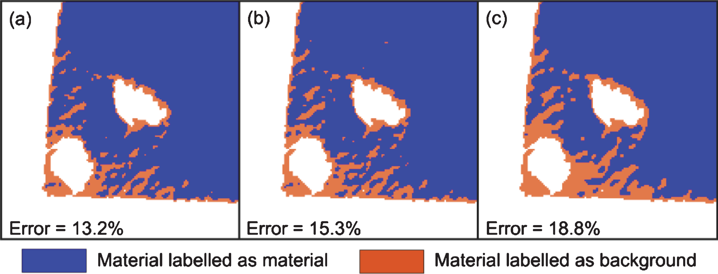
Otsu fails to segment correctly due to lack of a sharp valley in the global image histogram. ICM initialization and Otsu result are quite similar given both are global thresholding methods. The smoothing prior in the MRF method which is useful for correcting falsely detected pixels also smooths out the ‘fringes’, potentially connecting them by labelling material pixels as background.
4.2Titanium cuboid
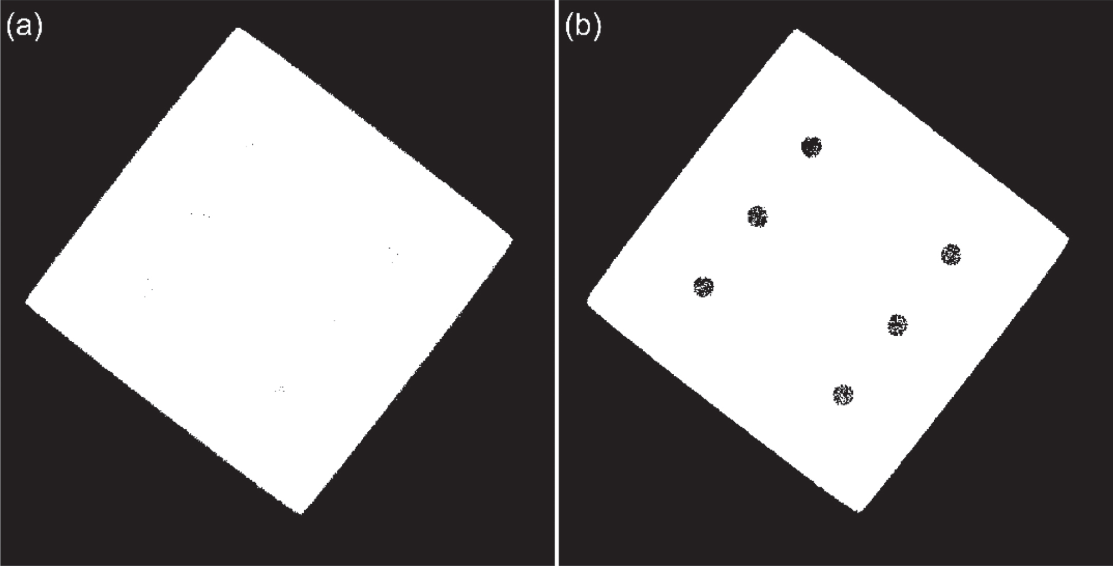
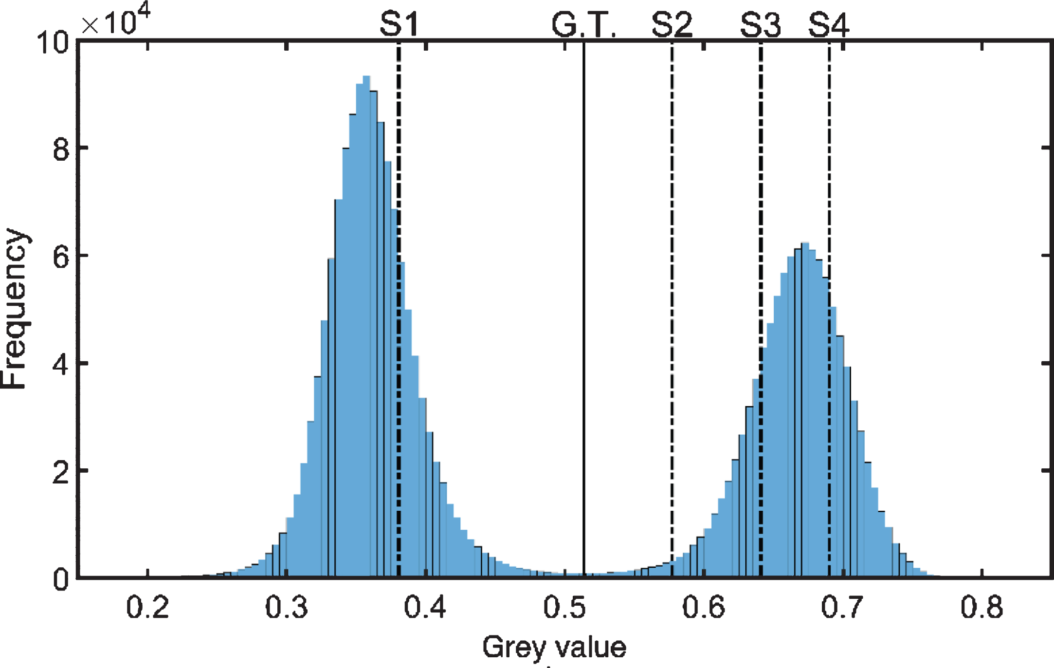
Results in Fig. 15 show that Otsu fails to segment the holes entirely whereas MRF detects the voids, although with noticeable grains of material assigned labels within the holes. The global threshold determined by Otsu is depicted as G.T. in image histogram in Fig. 16. It is observed that mean grey value of holes (area 2 in Fig. 7(b)) marked by S2, is on the material side of this threshold which is why Otsu labels them as such. Hole pixels are much fewer in number than material or rest of the background so they appear as a part of the material peak in image histogram, elongating its tail to the left. S1, S2, S3 and S4 indicate mean grey values of background, holes, the material at centre, and material near edge respectively from areas 1, 2, 3 and 4 marked in Fig. 7(b).
Segmentation of two important features in the titanium cuboid is shown in Fig. 17. ICM which is initialized by minimizing likelihood energy at each pixel shows irregular hole boundaries with several pixels assigned as material inside holes. As ICM converges, taking 5 iterations, the hole emerges clearer but still has some material within its boundary. The corner is more competently segmented by Otsu with the image quality causing the irregularities in its boundaries. MRF appears to hamper the shape of the corner by smoothing it and losing some material pixels to the background. Additionally, both approaches are affected by streak artefacts near the corners and as a result, have a tendency to chamfer the corner.
Fig.17
Two features from CT image in Fig. 7(a): (a) a hole and its Otsu segmentation, ICM initialization and MRF segmentation result in (b), (c) and (d) respectively, and (e) a corner and its Otsu segmentation, ICM initialization and MRF segmentation result in (f), (g) and (h) respectively. Note that methods are applied to the whole image and cropped sections are shown here.
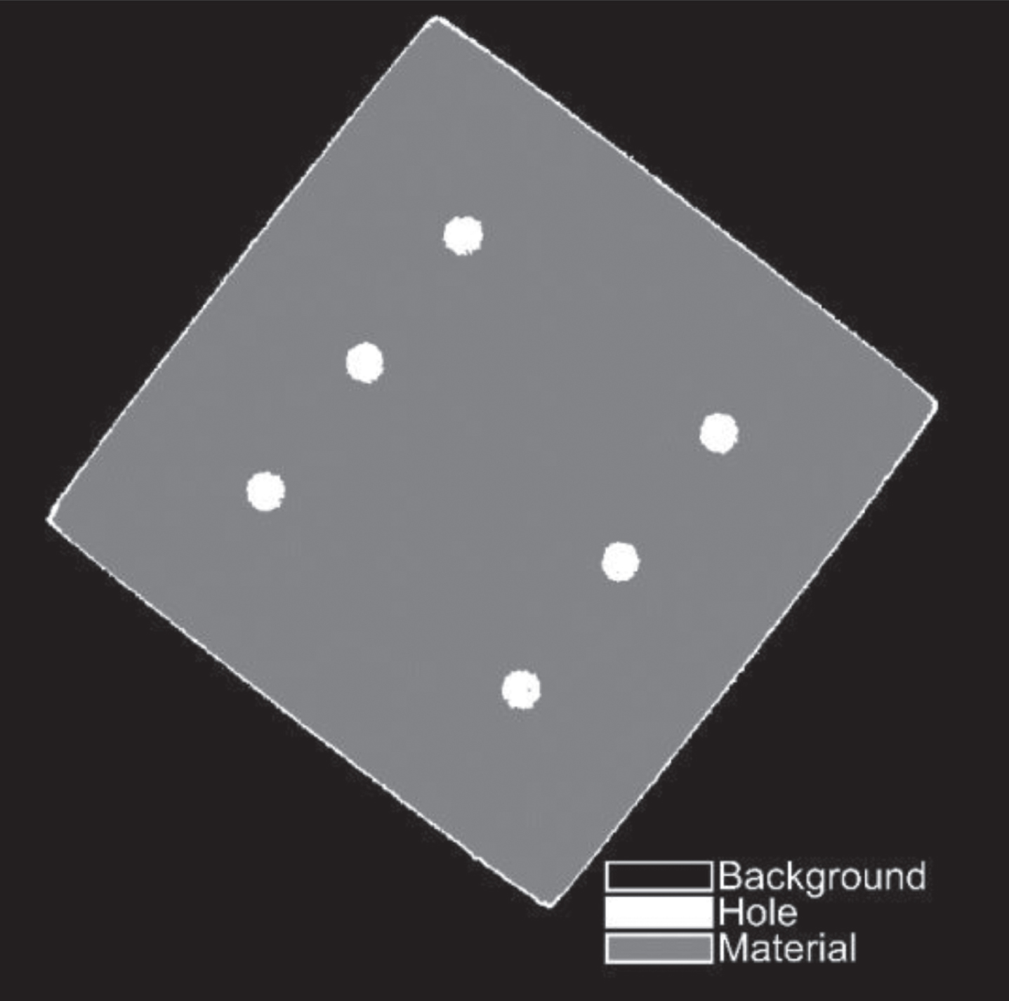
Since the grey value for holes is quantitatively different to the background, they can be considered as a different material in the object. Segmentations obtained for holes can then be combined with background to obtain the desired result. To assess its performance, MRF segmentation is applied with three labels instead of two and the result is shown in Fig. 18. It is observed that a thin layer a few pixels wide labelled hole material is formed around the object due to the transition in grey value across object boundary and partial volume effects.
Fig.18
MRF result for CT image in Fig. 7(a) with three labels- one each for background, material and holes affected by scatter.
It is observed that the holes are clearly segmented but the thin boundary around the object would hamper potential dimensional measurements involving object boundaries. To resolve this layer into material and background, prior knowledge about an object can be utilized. In object B, it is known that holes and background pixels are not neighbours. A constraint is introduced in ICM to prevent hole-background interactions after initialization in a large neighbourhood. A logical vector keeps track of pixels that were initialized as holes in areas of intermediate grey values between material and background. It prevents them from becoming reassigned as holes to avoid unnecessary iterations.
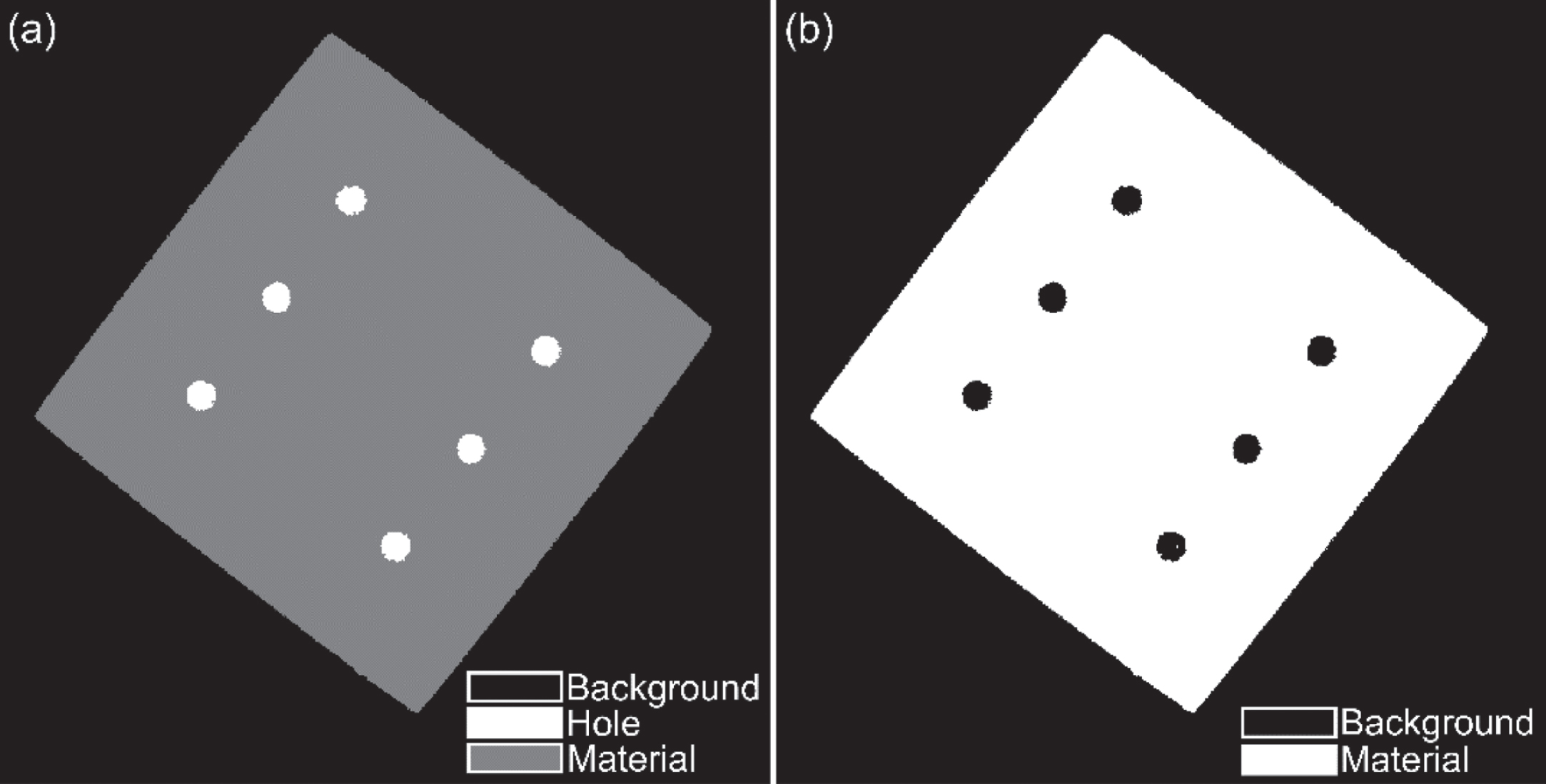
After ICM initialization, as the constraint is applied while making label changes, the thin layer gets resolved into its constituent background and material pixels. Figure 19 shows the performance of MRF segmentation after including the constraint to prevent hole-background neighbourhoods. This simple constraint is suitable for objects which have interior voids and holes entirely obscured by high scatter. ICM for both MRF 3 labels with and without constraint takes 11 iterations to converge.
Fig.19
For the titanium cuboid CT image in Fig. 7(a): (a) MRF segmentation output with 3 labels and the constraint to prevent forming of an imaginary layer of hole pixels on object boundary, and (b) final segmentation of the titanium cuboid.
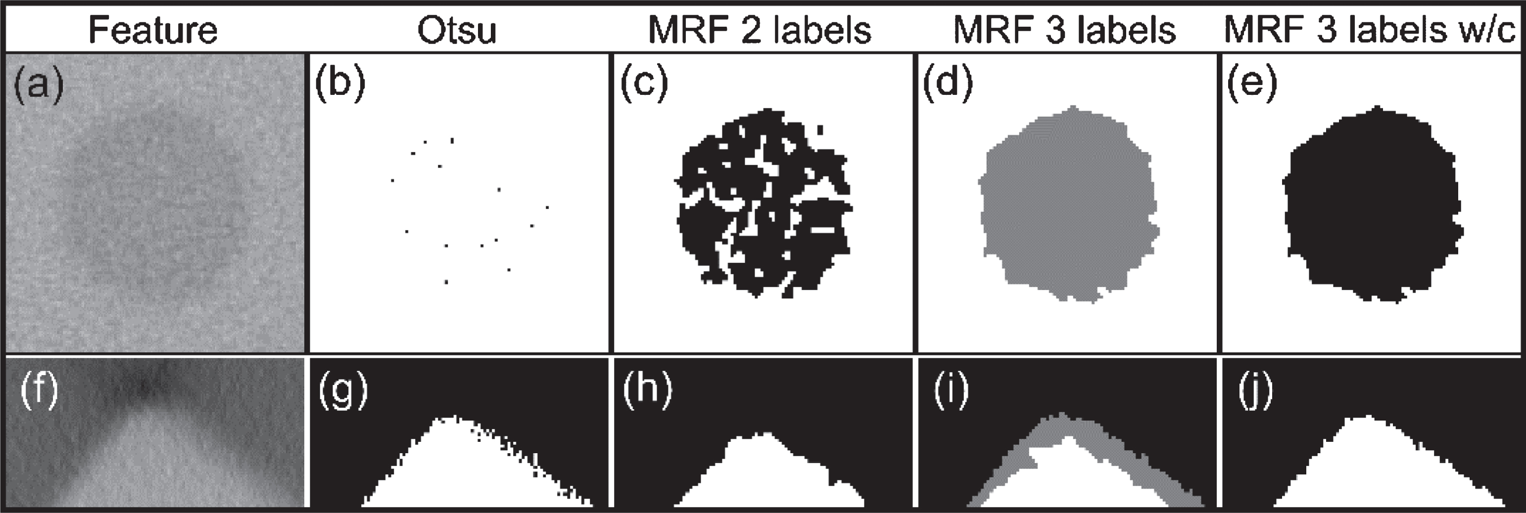
Otsu, MRF 2 labels, and MRF 3 labels segmentation results for features (a) and (e) in Fig. 17 are shown in Fig. 20. It is found that both holes and corners are very well resolved in MRF 3 labels. Corners are found to be correctly segmented like Otsu but significantly smoother. The reason for the correct segmentation of corners in MRF 3 labels, as opposed to MRF 2 labels, lies in ICM initialization where intermediate grey value pixels are assigned as hole and subsequently segmented as background and material due to the hole-background neighbourhood constraint in ICM.
Fig.20
Two features from CT image in Fig. 7(a): (a) a hole and (f) a corner with their (b, g) Otsu, (c, h) MRF 2 labels, (d, i) MRF 3 labels, and (e, j) MRF 3 labels with constraint segmentations respectively. Note that methods are applied to whole image and cropped sections are shown here.
5Conclusion
Otsu thresholding and Markov Random Field segmentation were applied to the reconstructed CT volume data sets of two objects: steel column and titanium cuboid. The highly attenuating nature of these materials promotes streaks, loss of contrast, blurred edges and noise making it difficult to segment. Further artefacts are generated from the object geometry leading to inhomogeneities in grey values.
Segmentation using MRF has significantly improved the segmentation of voids in the steel column sample. MRF segmentation shows notable results with highly obscured voids in the titanium cuboid whereas Otsu fails to detect any voids in the images. Analyzing CT data from the titanium cuboid particularly highlights MRF’s capabilities through incorporation of prior knowledge about an object. MRF with three labels and the additional constraint to prevent a layer of hole pixels around the periphery of the object, performs better than Otsu thresholding for both features: holes and corners.
However, non-uniform grey values and voids near corners in the steel column cause MRF to incorrectly assign some material pixels to background. Even Otsu fails to correctly segment the corner region as shown in Fig. 14(a) which suggests that objects with highly attenuating materials and sharp corners may always be problematic in XCT analysis, rather than an issue inherent to MRF. Further study in this domain will be crucial to understanding the material-geometry-segmentation relationship.
The comparison against Otsu was natural given its broad usage and identification as the main segmentation method in standards and best practice guides. It is clear that MRF has some significant advantages and warrants consideration as an alternative method in industrial XCT. Further, the wider array of segmentation techniques requires evaluation for specific cases that arise in industrial applications such as the review by Schluter et al. [39] for soil and porous media samples.
An extension to this work would be to apply the methodology to X-ray CT scans that show evidence of texture. Textures are not suitably segmented using traditional grey-scale methods such as Otsu as two textures could contain the same grey-scales but exhibit different patterns. Similarly, gradient based methods like watershed are clearly unsuitable. In this case a wavelet decomposition of the textures can be modelled with MRF with Gibbs cliques used for feature classification. This has been demonstrated for grey-scale images [40] that would be directly applicable to X-ray CT, and coloured textures [41] that is currently used in computer vision based applications. There are developments in ‘colour’ X-ray CT that identifies different materials by decomposing received spectra [42] for which this could potentially be of benefit. In this case the ground truth can be achieved through serial grinding of the sample and using scanning electron microscopy/energy dispersive spectroscopy (SEM/EDS) to achieve images for accuracy comparison.
To review, modelling a Markov random field to segment CT data influenced by scatter, streaks and noise can deliver appreciable results. MRF’s advantage in a segmentation task is that likelihood, and potential functions for prior can be changed for specific applications. Future work with metrological measurements and multi-material samples can aid to quantify and better assess MRF’s segmentation capabilities in XCT.
Acknowledgments
The authors would like to thank Stephen Spooner from WMG, University of Warwick and the Materials Processing Institute (MPI) for providing the steel samples.
References
[1] | De Chiffre L. , Carmignato S. , Kruth J-P , et al., Industrial applications of computed tomography, CIRP Annals - Manufacturing Technology 63: (2) ((2014) ), 655–677. |
[2] | Kruth J.P. , Bartscher M. , Carmignato S. et al., Computed tomography for dimensional metrology, CIRP Annals - Manufacturing Technology 60: (2) ((2011) ), 821–842. |
[3] | Landron C. , Maire E. , Adrien J. et al., Non-destructive 3-D reconstruction of the martensitic phase in a dual-phase steel using synchrotron holotomography, Scripta Materialia 66: (12) ((2012) ), 1077–1080. |
[4] | Maire E. and Withers P.J. , Quantitative X-ray tomography, International Materials Reviews 59: (1) ((2013) ), 1–43. |
[5] | Hiriyannaiah H.P. , X-ray computed tomography for medical imaging, IEEE Signal Processing Magazine 14: (2) ((1997) ), 42–59. |
[6] | Feldkamp L.A. , Davis L.C. and Kress J.W. , Practical cone-beam algorithm, Journal of the Optical Society of America A 1: (6) ((1984) ), 612–619. |
[7] | Müller P. , Hiller J. , Dai Y. et al., Quantitative analysis of scaling error compensation methods in dimensional X-ray computed tomography, CIRP Journal of Manufacturing Science and Technology 10: ((2015) ), 68–76. |
[8] | Bartscher M. , et al. Achieving traceability of industrial computed tomography, Proc. 9th Int. Symp. on Measurement and Intelligent Instruments, D.S. Rozhdestvensky Optical Society 1: ((2009) ), 256–261. |
[9] | Kumar J. , Attridge A. , Wood P.K.C. and Williams M.A. , Analysis of the effect of cone-beam geometry and test object configuration on the measurement accuracy of a computed tomography scanner used for dimensional measurement,, Measurement Science and Technology 22: (3) ((2011) ), 035105(15pp). |
[10] | Kueh A. , Warnett J.M. , Gibbons G.J. et al., Modelling the penumbra in computed tomography, Journal of X-Ray Science and Technology 24: (4) ((2016) ), 583–597. |
[11] | Kiekens K. , Welkenhuyzen F. , Tan Y. et al., A test object with parallel grooves for calibration and accuracy assessment of industrial computed tomography (CT) metrology, Measurement Science and Technology 22: (11) ((2011) ), 115502(7pp). |
[12] | Lifton J.J. , Malcolm A.A. and McBride J.W. , An experimental study on the influence of scatter and beam hardening in X-ray CT for dimensional metrology,, Measurement Science and Technology 27: (1) ((2015) ), 015007(12pp). |
[13] | Schörner K. , Development of methods for scatter artifact correction in industrial x-ray cone-beam computed tomography, Technical University of Munchen (2012) . |
[14] | Brooks R.A. and Di G. , Chiro, Beam hardening in x-ray reconstructive tomography, Physics in Medicine and Biology 21: (3) ((1976) ), 390. |
[15] | Siewerdsen J.H. and Jaffray D.A. , Cone-beam computed tomography with a flat-panel imager: Magnitude and effects of x-ray scatter, Medical Physics 28: (2) ((2001) ), 220–231. |
[16] | Park H.S. , Choi J.K. , Park K-R , et al., Metal artifact reduction in CT by identifying missing data hidden in metals, Journal of X-Ray Science and Technology 21: (3) ((2013) ), 357–372. |
[17] | Choi J. , Kim K.S. , Kim M.W. et al., Sparsity driven metal part reconstruction for artifact removal in dental CT, Journal of X-ray Science and Technology 19: (4) ((2011) ), 457–475. |
[18] | Verburg J.M. and Seco J. , CT metal artifact reduction method correcting for beam hardening and missing projections, Physics in Medicine and Biology 57: (9) ((2012) ), 2803–2818. |
[19] | Zhang X. , Wang J. and Xing L. , Metal artifact reduction in x-ray computed tomography (CT) by constrained optimization, Medical Physics 38: (2) ((2011) ), 701–711. |
[20] | Jeong K.Y. and Ra J.B. , Reduction of artifacts due to multiple metallic objects in computed tomography, Medical Imaging 2009: Physics of Medical Imaging 7258: (1) ((2009) ), 72583E. |
[21] | Mouton A. , Megherbi N. , Slambrouck K.V. et al., An experimental survey of metal artefact reduction in computed tomography, Journal of X-ray Science and Technology 21: (2) ((2013) ), 193–226. |
[22] | Otsu N. , A threshold selection method from grey-level histograms, IEEE Transactions on Systems, Man, and Cybernetics 9: (1) ((1979) ), 62–66. |
[23] | British Standards Institution, BS 16016 ((2011) ). |
[24] | Sun W. , Brown S.B. and Leach R.K. , An overview of industrial x-ray computed tomography, NPL Report ENG 32: , (2012) . |
[25] | Carmignato S. , Accuracy of industrial computed tomography measurements: Experimental results from an international comparison, CIRP Annals – Manufacturing Technology 61: (1) ((2012) ), 491–494. |
[26] | Vincent L. and Soille P. , Watershed in digital spaces: An efficient algorithm based on immersion simulations, IEEE Transactions on Pattern Analysis and Machine Intelligence 6: ((1991) ), 583–598. |
[27] | Shammaa M.H. , Ohtake Y. and Suzuki H. , Segmentation of multi-material CT data of mechanical parts for extracting boundary surfaces, Computer-Aided Design 42: (2), 118–128. |
[28] | Li S.Z. , Markov random field modeling in image analysis. 3rd ed. London: Springer, (2010) . |
[29] | Besag J. , On the statistical-analysis of dirty pictures, Journal of the Royal Statistical Society, Series B (Methodological) 48: (3) ((1986) ), 259–302. |
[30] | Zhang Y. , Brady M. and Smith S. , Segmentation of brain MR images through a hidden Markov random field model and the expectation-maximization algorithm, IEEE Transactions on Medical Imaging 20: (1) ((2001) ), 45–57. |
[31] | Li M. , Zheng J. , Zhang T. et al., A prior-based metal artifact reduction algorithm for x-ray CT, Journal of X-ray Science and Technology 23: (2) ((2015) ), 229–241. |
[32] | Hermanek P. and Carmignato S. , Reference object for evaluating the accuracy of porosity measurements by X-ray computed tomography, Case Studies in Nondestructive Testing and Evaluation 6: (B) ((2016) ), 122–127. |
[33] | Geman S. and Geman D. , Stochastic relaxation Gibbs distributions and the Bayesian restoration of images, IEEE Transactions on Pattern Analysis and Machine Intelligence 6: (6) ((1984) ), 721–741. |
[34] | Besag J. , Spatial interaction and the statistical analysis of lattice systems, Journal of the Royal Statistical Society 36: (2) ((1974) ), 192–236. |
[35] | Derin H. and Elliott H. , Modeling and segmentation of noisy and textured images using Gibbs random fields, IEEE Transactions On Pattern Analysis And Machine Intelligence 9: (1) ((1987) ), 39–55. |
[36] | Huang F. , Narayan S. , Wilson D. et al., A fast iterated conditional modes algorithm for water-fat decomposition in MRI, IEEE Transactions on Medical Imaging 30: (8) ((2011) ), 1480–1492. |
[37] | Herman G.T. , Correction for beam hardening in computed tomography, Physics in Medicine and Biology 24: (1) ((1979) ), 81. |
[38] | Veldkamp W.J.H. , Joemai R.M.S. , van der Molen A.J. and Geleijns J. , Development and validation of segmentation and interpolation techniques in sinograms for metal artifact suppression in CT, Medical Physics 37: (2) ((2010) ), 620–628. |
[39] | Schluter S. , Sheppard A. , Brown K. and Wildenschild D. , Image processing of multiphase images obtained via X-ray microtomography: A review, Water Resources Research 50: (4) ((2014) ), 3615–3639. |
[40] | Wang L. and Liu J. , Texture classification using multi resolution Markov random field models, Pattern Recognition Letters 20: (2) ((1999) ), 171–182. |
[41] | Chen M. and Strobl J. , Multispectral textured image segmentation using a multi-resolution fuxxy Markov random field model on variable scales in the wavelet domain, International Journal of Remote Sensing 34: (13) ((2013) ), 4550–4569. |
[42] | Egan C.K. , Jacques S.D. , Wilson M.D. et al., 3D chemical imaging in the laboratory by hyperspectral X-ray computed tomography, Scientific Reports 5: ((2015) ), 15979. |


