
The nature of regional bias in Heisman voting
Abstract
This study explores regional bias in Heisman voting from 1990–2016 using a negative binomial regression model with player-year fixed effects. Analysis confirms finalists receive higher vote tallies in home regions, on average. Additionally, results show regional vote tallies are decreasing in the fraction of other finalists in-region. Furthermore, evidence reveals finalists receive higher vote tallies for each game played against in-region teams and lower vote tallies for each game played by other finalists against in-region teams. Analysis is augmented by showing the recent increase in national television coverage of college football has been accompanied by a decline in regional bias.
1Introduction
1.1Media accounts of regional bias
The Heisman Trophy is the utmost individual accolade a college football player can have bestowed upon him. According to former University of Florida and University of South Carolina head coach and 1966 Heisman Trophy winner Steve Spurrier (2012), the Heisman Trophy is “the single greatest award in all of amateur sports.” Others have gone as far as calling it “the single most celebrated award in … American sports (Heisman & Schlabach, 2012)” and “America’s most famous individual sports award (Alzo & Oxenreiter, 2007).”
Despite the fact the Heisman Trophy is one of the most prestigious honors in American sports, there has been wide-spread media speculation of the existence of a strong regional bias in voting almost as long as the award has existed. However, the nature of such bias has been an issue for debate. For instance, in the first 31 years the Heisman Trophy was awarded only twice did it go to a player in the South, which at the time led some to claim regional bias against Southern players (Outside the Sidelines, 2007). In the early-1970s Joe Falls of the Detroit Free Press noted “I think there’s a natural resentment against … the east, in the Midwest and the far west (Jacobson, 1971).”
More recently analysts have speculated about bias against the Far West. For example, New York Times writer Joe Drape has noted that players from the Far West need “more inflated statistics to overcome the obscurity that players from the West Coast generally toil in (Drape, 2001)” and Heisman-winning quarterback Jim Plunkett has stated “there’s definitely an eastern and southern bias to the voting (Wilner, 2009).” Many journalists have suggested regional bias against players from the Far West is a function of voters being unable to watch games on the west coast that are broadcast into the late evening hours on the east coast; there is also arguably less cultural interest in and less television coverage of teams in the Far West. By one account, a Heisman voter and very prominent former coach once admitted to never having seen a specific Far West candidate in action (Horne, 2013).
According to the Heisman Trophy website, “Heisman voters are dispersed across the various regions with the goal of reducing the likelihood of regional bias being a factor in the final outcome(Huston, 2016).” However, it is worth noting that “structural regional bias” may negatively impact Far West candidates since the Far West contains the largest fraction of the United States (US) population among the six regions but the allotment of regional votes is not representative of the population size (Chisolm, 2003). Bias against players in the Far West may be evidenced by the fact that in the 82 years of the award only five Far West players from schools other than the University of Southern California have won the award (Heisman, 2017).
Still, others have remarked that “people tend to watch and vote for what’s in front of them,” suggesting that voters are more likely to vote for candidates who play in their region (Weinreb, 2016). However, others have noted that “now games are on TV from morning until midnight on Saturday,” suggesting that increased personal knowledge of Heisman finalists may eventually result in an end to regional bias in Heisman voting (The Oklahoman, 2003).
1.2Heisman trophy voting
Since 1977 there have been six Heisman regions (Northeast, Mid-Atlantic, South, Southwest, Midwest, and Far West), and each region is allotted 145 votes to distribute among media members (Heisman, 2014; McCartney, 2016). The selection of voters is determined via a complex process that involves selection of individual voters by state representatives appointed by the regional representative overseeing their state (Heisman, 2014). The number of votes allotted a state depends both on the size of the state and the number of media outlets contained within. All living former Heisman winners (58 as of 2016) are also permitted to vote and their votes are distributed among the six regions in the final tabulation(Heisman, 2014). Since 1999, fans in aggregate have also been allotted one vote via online polling (Heisman, 2014).
Voting for the award takes place after all regular season and conference championship games have been played but before bowl season begins. For a voter’s ballot to count, he or she must specify a first-, second-, and third-place choice (Heisman, 2014). Once ballots have been received results are tabulated by the accounting firm Deloitte and aggregate tallies are determined awarding each voter’s first selection three points, second selection two points, and third selection one point (Heisman, 2014). The number of finalists vary by year and are determined by the final vote tally; there will always be at least three finalists and additional finalists are invited if their point totals are relatively close to that of the third-place finisher (Heisman, 2014). Regional tallies are only released for finalists who are invited to attend the Heisman ceremony (McCartney, 2016).
1.3Connections to previous studies
Despite widespread media speculation on the nature of regional bias in Heisman voting, there has not been a peer-reviewed academic study verifying the existence of regional bias in Heisman voting nor commenting on the nature of such bias. In addition, there have only been a few quantitative inquiries into the subject by news media and academics, and none of these attempts are nearly as academically rigorous as the analysis presented in this article.
In one study, Haptonstall (2005) analyzed an anonymous survey completed by Heisman voters in reference to the 2003 Heisman race. In the survey, voters were asked (1) which candidates they voted for, (2) whether they tend to vote for players from their own region as their top selection, and (3) whether they believe most voters choose players from their own region as their top selection. Using this survey, Haptonstall (2005) determined that each of the top four candidates in the 2003 Heisman race received a disproportionate number of votes from voters within his geographic region. In addition, voters taking the survey indicated disagreement that they had a tendency to vote for players from their region but leaned toward agreement that other voters had such tendency. Thus, voters generally believe they have an open mind as to which player they vote for but perceive that others do not (Haptonstall, 2005).
In another analysis, Donchess (2014) used Heisman races from 2009–2013 to compare regional vote tallies for each finalist to the finalist’s average tally across all six regions. Donchess (2014) found heavy bias in the Far West and South regions that was roughly three times worse than the bias found in the Mid-Atlantic region. He theorizes this is the joint impact of (1) media members in the South and Far West being more myopic and (2) other regions having fewer Heisman candidates and thus less reason to be partial (Donchess, 2014). According to Knox and Grossman (2015), nine of the top ten instances of regional bias (as measured by a finalist’s percent difference in the points earned in an individual region and the average points per region across all six regions) between 1998 and 2014 come from a player’s home region, and the South, Southwest, and Midwest combined showed the largest bias in a season in 12 of the 17 years studied. A count of votes for the top ten offensive Heisman candidates from 2000–2009 shows that players from the Mid-Atlantic, Midwest, Northeast, and Far West regions tend to receive fewer vote tallies than candidates in the South or Southwest regions, though this analysis does not take into account the merit of the candidates (Heard, 2013).
This study dramatically improves upon the methodology employed in previous examinations and greatly expands the universe of data employed. Using regional data on Heisman finalists from 1990–2016, this analysis explores the nature of regional bias in Heisman voting with an unconditional fixed-effects negative binomial regression (NB2) model that includes indicator variables to represent player-year fixed effects. In accordance with Donchess (2014), Haptonstall (2005), and Knox and Grossman (2015), the analysis shows that Heisman finalists receive higher vote tallies in their home regions. Additionally, the analysis further shows that regional vote tallies are positively associated with the number of games finalists played against teams based within-region, as hinted at as a possibility by Knox and Grossman (2015).
This study also finds suggestive evidence that same-region bias is larger in the Northeast, South, Southwest, and Far West than in the Mid-Atlantic and Midwest, advancing the analysis by Donchess (2014) and Knox and Grossman (2015). However, contrary to evidence presented in Heard (2013), the well-identified analysis presented here finds no evidence that finalists from the Mid-Atlantic, Midwest, or Far West receive lower vote tallies in other regions compared to other out-of-region finalists; conversely, evidence suggests finalists from the Northeast, South, and Southwest are more likely to be treated adversely in other regions. This study also expands upon previous analyses by showing that regional vote tallies are negatively associated with the fraction of other finalists based within-region and the number of games played by other finalists against teams based within-region. Furthermore, the results indicate that an increase in national television coverage of college football games has been accompanied by a decrease in regional bias.
Such results fit firmly into the broader social science literature regarding voting behavior and the neighborhood effect, whereby the concentration of votes for a given candidate is larger than expected. Spatial correlation in voting behavior comes about due to commonality in experiences and information flows in an individual’s local environment, which in this case may come about based on more similar television and news content within-region as compared to across regions (Cox, 1969; Johnston, 1986). Moreover, such local biases will be deepened by further interactions with others receiving the same biased information, such as interactions with fans and other media members within-region (Burbank, 1995; Fitton, 1973; Pattie & Johnston, 2000; Taylor & Johnson, 1979). Such bias may be further intensified due to misplaced support for the local candidate based strictly on emotion rather than information (Curtice & Steed, 1982; Johnston, 1983).
1.4Evidence from specific Heisman races over three decades
A number of hypotheses can be gleaned from a brief introspection of specific Heisman races. For instance, in the 1993 Heisman race the second-, third-, fourth-, and fifth-place finishers all received a significantly greater number of votes in their home regions. Only the first-place finisher, Charlie Ward of Florida State, received more votes in regions outside of his home region. One is free to speculate about why Charlie Ward received fewer votes in the South than in the Mid-Atlantic, Southwest, Midwest, and Far West, but it is likely a combination of the fact that the second- and third-place finalists also came from Southern universities (Heath Shuler of Tennessee and David Palmer of Alabama), Florida State played the majority of their games in the Mid-Atlantic region (7), and Florida State had a significant national advantage based on their television broadcast schedule as compared to the other four finalists.
Similarly, in the 2001 Heisman race, the first-, second-, and fourth-place finishers all received significantly larger vote tallies in their home regions. The third-place finisher, Ken Dorsey of Miami, received fewer votes in his home region, the South, than in the Northeast, Mid-Atlantic, or Far West regions. This may be unsurprising as Dorsey, like Ward in 1993, also played the majority of his games in the Mid-Atlantic region (6) and also faced another finalist from the South (Rex Grossman of Florida). Additionally, Dorsey played two games against universities located in the Northeast while the other three finalists combined played none— voters in the Northeast overwhelmingly voted for him without an alternative finalist from their region.
The 2014 Heisman race was the first time in 44 years where a player from the Pacific Time Zone attending a university other than the University of Southern California won the award. What is interesting about 2014 is that it is the first year in which the whole schedule of games for all finalists were nationally televised. This is due to the relatively recent increase in the number of national channels carrying weekly college football games, especially among networks devoted to a single conference such as the Big Ten Network, Pac-12 Network, and SEC Network. What is quite noticeable in this case is that, while each finalist received the most votes within his home region, the average percent difference between vote tallies in each finalist’s home region and the other five regions is significantly lower in the 2014 race than in the 2001 or 1993 race. Though much more introspection is clearly necessary, the dramatic decline in the average percent difference between vote tallies in each finalist’s home region and the other five regions from 1993 to 2001 and 2001 to 2014 reveals the possibility there may be some role of national television coverage in attenuating regional bias.
1.5Theoretical expectations
Based on findings from the literature and anecdotal evidence presented above, theory dictates that a finalist’s vote tally in a given region has the potential to be influenced by the region in which the finalist’s university is based. While one may expect to find the strongest observed impact of regional bias when the finalist and voters are based in the same region, there is also the potential that vote tallies for finalists based in nearby regions will be greater than for finalists based further away. For example, one may expect that a finalist based in the Mid-Atlantic region will receive a higher vote tally from voters in the Northeast region than from voters in the Far West region. The expected impact of the intersection of player region and voter region may be lessened when many finalists are based in the same or nearby regions. For instance, if more than one finalist is based in a single region the regional vote may be split among the in-region finalists, but if only one finalist is based in-region he may receive the lion’s share of regional votes.
One should also expect that any factor that would impact one finalist will have the opposite effect on one or more other finalists since the vote share is zero-sum. This suggests that when there are one or more finalists from or in close proximity to a given region that other finalists may receive lower vote tallies from voters based in that particular region, on average. Moreover, the more finalists based in or near a particular region, the lower one might expect other finalists’ vote tallies from that particular region will be.
From the examples discussed in the last subsection, it appears the location of a finalist’s opponents also plays a factor in regional vote tallies. This appears noticeably true in many other cases not discussed, especially in cases where a finalist is based in one region but plays in a conference where the majority of opponents are located in another region. Therefore, one may expect a ceteris paribus positive relationship between the vote tally a player receives from voters in a particular region and the number of games he plays against opponents based in the region. Likewise, since voting is a zero-sum game, one may also expect a ceteris paribus negative relationship between a finalist’s regional vote tally and the number of games other finalists play against opponents based in that region.
Observing the examples examined in the previous subsection, it also appears the expansion of national television coverage of college football games has had a substantial impact on the pervasiveness of regional bias. The average percent difference across all finalists between the vote tally a finalist received in his home region and the average vote tally across all other regions, referred to in Table 1 as Percent Bias, fell from 123.1% in 1993 to 33.1% in 2014 as television coverage increased substantially. Figure 1, which shows the Average National TV, the average number of games finalists played on national television, and the Average Percent Bias for five year periods between 1990 and 2014, reveals this trend is in no way specific to the examples provided. In each five year period shown between 1990 and 2014 average percent bias ticked downward while national television coverage of finalists generally increased.
Fig.1
National television coverage and average percent bias, 1990–2014. Notes: Data from five year periods from 1990–2014 were used to produce this graph. The graph shows the average national television coverage and average percent bias of Heisman finalists over five year periods starting in 1990 and ending in 2014. The graph makes it clear there has been a substantial increase in national television coverage of finalists over this time period that coincides with a rather steep decline in average percent bias. This reveals the possibility that national television coverage may play some role in attenuating regional bias.
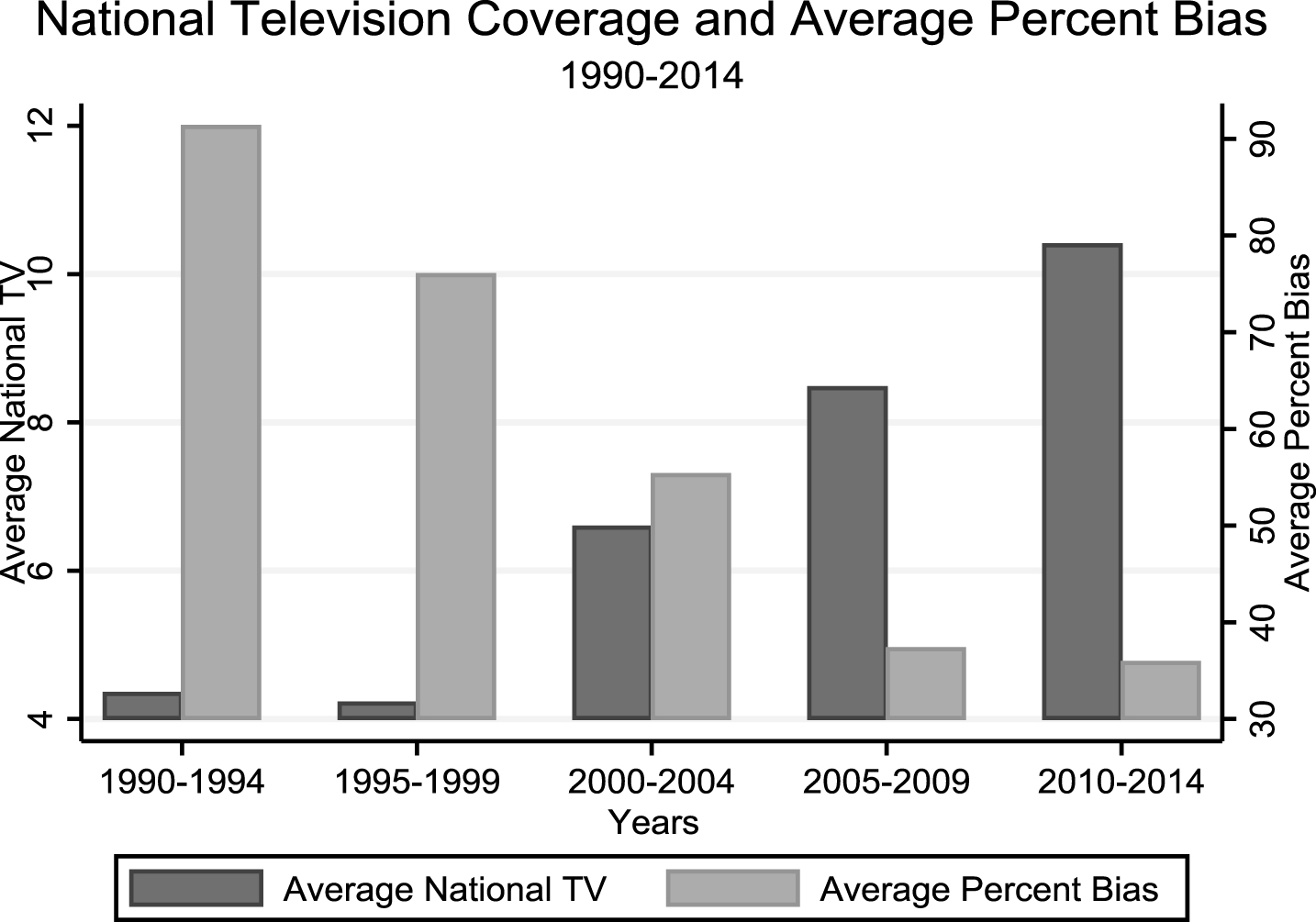
Table 1
The nature of regional bias in three specific Heisman races
| Panel A. 1993 Heisman Race | |||||||||
|---|---|---|---|---|---|---|---|---|---|
| Player | School | Position | Northeast | Mid-Atlantic | South | Southwest | Midwest | Far West | Percent Bias |
| Charlie Ward | Florida State | QB | 371 | 388 | 373† | 408 | 380 | 390 | – 3.7% |
| Heath Shuler | Tennessee | QB | 81 | 132 | 157† | 122 | 103 | 93 | 47.8% |
| David Palmer | Alabama | RB | 34 | 55 | 97† | 50 | 26 | 30 | 148.7% |
| Marshall Faulk | San Diego State | RB | 39 | 34 | 21 | 39 | 33 | 74† | 122.9% |
| Glenn Foley | Boston College | QB | 80† | 49 | 5 | 13 | 21 | 12 | 300.0% |
| Panel B. 2001 Heisman Race | |||||||||
| Player | School | Position | Northeast | Mid-Atlantic | South | Southwest | Midwest | Far West | Percent Bias |
| Eric Crouch | Nebraska | QB | 159 | 103 | 79 | 204† | 103 | 122 | 80.2% |
| Rex Grossman | Florida | QB | 121 | 171 | 180† | 65 | 78 | 93 | 70.5% |
| Ken Dorsey | Miami (FL) | QB | 179 | 128 | 92† | 77 | 64 | 98 | – 15.8% |
| Joey Harrington | Oregon | QB | 62 | 41 | 50 | 39 | 35 | 137† | 201.8% |
| Panel C. 2014 Heisman Race | |||||||||
| Player | School | Position | Northeast | Mid-Atlantic | South | Southwest | Midwest | Far West | Percent Bias |
| Marcus Mariota | Oregon | QB | 409 | 410 | 426 | 434 | 420 | 435† | 3.6% |
| Melvin Gordon | Wisconsin | RB | 201 | 208 | 167 | 198 | 256† | 220 | 28.8% |
| Amari Cooper | Alabama | WR | 150 | 184 | 256† | 173 | 121 | 139 | 66.9% |
Notes: Each player’s home region is indicated by†. Percent bias is calculated as the difference between the number of votes in a player’s home region and the average number of votes across all other regions divided by the latter.
Theory suggests that the more widespread the coverage is for a particular finalist, the lower the difference will be between the vote tally in the finalist’s home region and his vote tallies in all other regions. Likewise, more widespread national coverage of finalists based outside a given finalist’s home region may increase the number of votes for those finalists in that region, thereby decreasing the given finalist’s in-region vote share. One may also expect more national coverage to decrease the importance of the location of one’s scheduled opponents, as the finalist will be more visible in a given region regardless of whether or not he plays opponents based there. Similarly, more widespread national television coverage of other finalists may also decrease the importance of their playingopponents’ locations.
2Data and methodology
2.1Data sources and variables
The data used in this study comes from a multitude of sources. Regional vote tallies for Heisman finalists from 1990–2016 are collected from Associated Press releases in US newspapers. Each finalist’s home region is determined using the location of his university and delineation of Heisman regions defined by the Heisman Trust (Heisman, 2014). For each finalist, the regional distribution of opposing teams (those on the playing schedule prior to the Heisman announcement) is determined using the delineation of Heisman regions and schedule of each finalist’s university found on the Sports Reference website (www.sports-reference.com). National television broadcast schedules prior to the year 2000 are determined using past broadcast television information found on the 506 Sports website (506Sports.com) and cable television information provided in previous issues of the New York Times. From the year 2000 on, television broadcast schedules are appropriated from the National Champs website (NationalChamps.net).
In the data collected, each observation represents an observation for player i in region j in year t. Based on the information gathering process described above, variables are formed corresponding to the vote tally for player i in region j in year t (Region Tally = RTi,j,t), an indicator variable taking the value 1 if finalist i’s university was based in region j in year t and taking the value 0 otherwise (Player in Region = PiRi,j,t), and the fraction of finalists other than finalist i whose universities were based in region j in year t (Fraction Other Finalists in Region = FOFiRi′,j,t). The fraction of other finalists, as opposed to the raw number of other finalists, whose universities were based in region j in year t was used in this study to reflect the fact that the number of finalists in the voter region may have a different impact on regional vote tallies dependent upon the total number of finalists in a given year, which varies. Using the fraction instead of the raw number adds a very modest amount of explanatory power in the full model specified in Equation 1 but does not substantively change any of the results of the analysis. Playing schedule information described above is used to determine the number of games finalist i’s university played against teams based in region j in year t prior to the Heisman announcement (Opposing Teams in Region = OTiRi,j,t) and the average of this variable over all finalists other than finalist i in region j in year t (Finalists Avg. Opposing Teams in Region = FAOTiRi′,j,t).
Using the data collected corresponding to television broadcast schedules, a variable is created describing the number of nationally televised games played by finalist i in year t (National TV = NTVi,t). This variable includes all games on broadcast television (ABC, CBS, NBC, FOX) and major, nationally-syndicated cable stations (ESPN, ESPN2, ESPN-U, ESPN News, FX, and TBS, and later ACC Network, Big Ten Network, CBS Sports Network/CSTV, Fox Sports 1, NBC Sports Network/Versus, Pac-12 Network, SEC Network); games shown on a multitude of Fox Sports Network regional affiliates are also included. For widespread regional coverage (in which between two to five games are shown countrywide, as has been quite prevalent in ABC’s college football coverage), each game is counted as a fraction of the total number of regional games shown on that station in that timeslot. The average value of this variable over all finalists other than finalist i in year t (Other Finalists National TV = OtFNTVi′,t) and over all finalists other than finalist i whose university is based outside of region j in year t (Outside Finalists National TV = OuFNTVi′,j′,t) are also determined.
2.2Summary statistics
Table 2 shows summary statistics describing the dataset discussed in the last subsection for the full sample and for subsamples where the finalist is based within-region and out-of-region. Each observation in the data is weighted by the inverse of the number of finalists in year t so that all years are weighted equally in the analysis. In addition, the statistical significance of each difference across within-region and out-of-region subsamples is tested at the 1%, 5%, and 10% significance levels using chi-squared tests. On average, each finalist receives a regional vote tally of approximately 174 points. However, this varies significantly depending on whether the player is based in-region — when the player is based in-region he receives a tally of approximately 221 points but when he is based out-of-region he receives approximately 165 points, a difference that is statistically significant (P < 0.01).
Table 2
Summary statistics describing the nature of regional bias, 1990–2016
| Full Sample | In Region | Out of Region | Differences | |||||||
|---|---|---|---|---|---|---|---|---|---|---|
| Variable | Mean | Std. Dev. | Mean | Std. Dev. | Mean | Std. Dev. | Mean | Std. Err. | Chi-Sq | P-value |
| Player in Region | 0.17 | 0.37 | ||||||||
| Region Tally | 173.87 | 110.57 | 220.61 | 110.60 | 164.53 | 108.26 | 56.08 | 11.47 | 23.92 | <0.001 |
| Fraction Other Finalists in Region | 0.17 | 0.22 | 0.19 | 0.20 | 0.16 | 0.22 | 0.03 | 0.02 | 1.38 | 0.240 |
| Opposing Teams in Region | 1.98 | 3.00 | 7.25 | 2.91 | 0.93 | 1.57 | 6.32 | 0.28 | 502.72 | <0.001 |
| Finalists Avg. Opposing Teams in Region | 1.98 | 1.79 | 2.15 | 1.67 | 1.95 | 1.81 | 0.20 | 0.18 | 1.2 | 0.274 |
| Nationally Televised Games | 7.21 | 3.31 | ||||||||
| Obs | 708 | 118 | 590 | 708 | ||||||
Notes: Differences between ‘in region’ and ‘out of region’ samples exist at the 1% level among ‘region tally’ and ‘opposing teams in region.’ Differences in ‘region tally,’ ‘opposing teams in region,’ and ‘finalists avg. opposing teams in region’ are estimated from separate negative binomial regressions that include the ‘in region’ indicator as a regressor, while the difference in the ‘fraction other finalists in region’ is estimated from a least squared regression that includes the ‘in region’ indicator as a regressor.
As one might expect, on average each finalist also plays more games against teams within his region: a player plays an average of 7.25 games against teams in his region but plays less than 2 games on average against teams in each other region. The difference between the number of games a finalist plays against teams in a region depending on whether he is or is not based in-region is also statistically significant (P < 0.01). Average differences grounded in whether a finalist is based in-region for the fraction of other finalists in-region and other finalists’ average opposing teams in-region appear superficial and not statistically meaningful.
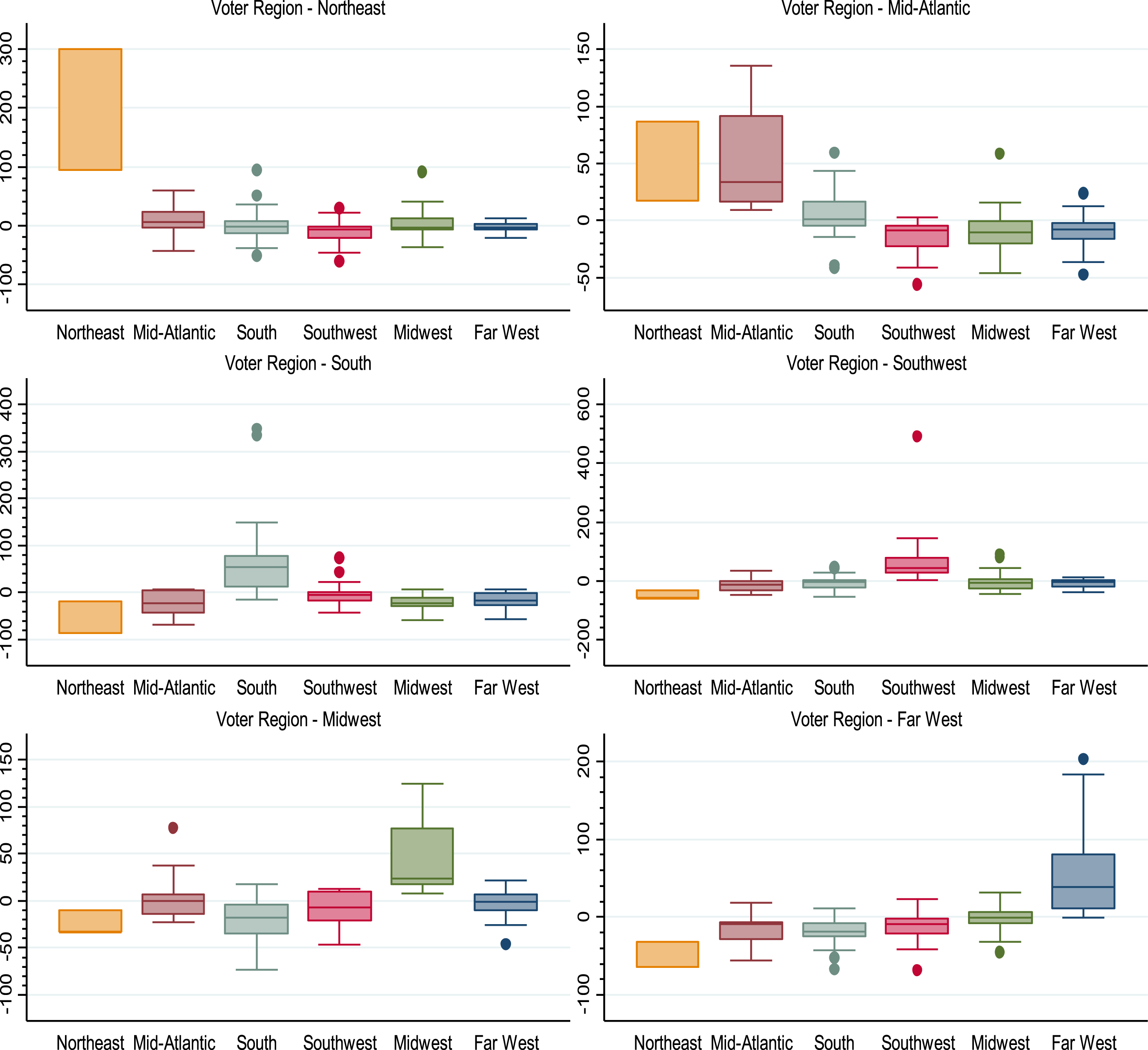
Boxplots of Percent Bias by voter region specific to the region where the finalist is based are shown in Fig. 2. What is most clear from the six boxplots is the dramatic extent of same-region bias in vote tallies. In all regions, the 25th percentile of Percent Bias for finalists based within-region is above or close to being above the 75th percentile for finalists based in each other region. Other noteworthy distributional differences exist, particularly as it pertains to finalists from the Northeast being somewhat more likely than finalists from other regions to receive votes in the Mid-Atlantic region and somewhat less likely than finalists from other regions to receive votes in the other four regions. In the Mid-Atlantic region, finalists from the South are also more likely to receive votes than those from the Southwest, Midwest, or Far West, as was seen in specific examples presented in Section 1.4. In the Midwest, finalists from the South are also slightly less likely to receive votes than finalists from the Mid-Atlantic, Southwest, or Far West, and in the Far West finalists from the Midwest are slightly more likely to receive votes than finalists from the Mid-Atlantic, South, or Southwest.
Fig.2
Cross-region voting differences, 1990–2016. Notes: Each graph shows percent bias on the y-axis and player region on the x-axis. There are too few observations of finalists from the Northeast region to calculate all the necessary descriptive statistics. Thus, the boxplots for finalists from the Northeast region only display the range of observations. What is most evident in this figure is the dramatic extent of same-region bias. In nearly all regions, the 25th percentile of percent bias for finalists based within the region is above or close to being above the 75th percentile for finalists based in each other region.
2.3The empirical model
Regional vote tallies for Heisman finalists are released but the ballots of individual voters are not. This rules out the use of a discrete choice model such as the multinomial logistic regression model since the number of ballots on which one finalist is selected over another in each region is unobserved. This also rules out models such as the ordered probit regression model or ordered logistic regression model that use the ordering of finalists on each ballot as the outcome variable. Introspection of the distribution of Region Tally reveals that regional vote tallies are discrete count data and the distribution is skewed such that the minority of finalists receive the majority of votes. Thus, linear regression would be a poor choice since it assumes continuous and normally distributed error terms and may produce negative predicted values, which are theoretically impossible. Additionally, the summary statistics reveal that overdispersion in Region Tally is likely since its variance is over 70 times larger than its mean. This rules out the use of the Poisson regression model. Additionally, an overdispersed Poisson regression model would also be a poor choice for inference since the variance of the outcome variable is so large as compared to its mean. The combination of these factors led to the use of a negative binomial regression model in order to deal with skewed, discrete count data with likely overdispersion in theerror term.
Since the negative binomial regression model will be used to analyze regional vote tallies, it is assumed
More specifically, the NB2 regression model to be estimated takes the general form
(1)
In this model, δ is the player-year indicator variable specific to player i in year t and γ is a region-specific indicator; for each, one category is selected as the baseline to allow for estimation. All other variables are as previously described.
Model coefficients are identified based on the covariation in the outcome variable Region Tally with the various input variables across region within player and year. First, a simplified version of Equation 1 including only Player in Region, Fraction Other Finalists in Region, an interaction term between the two, and player-year and region fixed-effects is estimated that does not account for the locations of finalists’ playing opponents. This equation takes the form
The interaction between Player in Region and Fraction Other Finalists in Region is included to allow the impact of Fraction Other Finalists in Region to vary dependent upon whether finalist i is based within-region; one might expect the fraction of other finalists in-region to have a larger impact on a within-region finalist since the total fraction of finalists from within-region will be larger in this case. The hypotheses discussed earlier suggest β1 > 0, β2 < 0, and β3 < 0.
Then, Opposing Teams in Region and Finalists Avg. Opposing Teams in Region are added to separate the impact of a finalist’s region from that of opponents on his schedule. This equation takes the form
In addition to the aforementioned expectations, hypotheses suggest β4 > 0 and β5 < 0.
Next, national television schedules are incorporated into the analysis by re-estimating Equation 1a with the added interaction terms Player in Region * National TV and Fraction Other Finalists in Region * Outside Finalists National TV. The coefficients on these interaction terms will have the same magnitude as interactions between Player Outside of Region * National TV and Fraction Other Finalists Outside of Region * Outside Finalists National TV, where Player Outside of Region is defined as an indicator variable taking the value 0 if finalist i’s university was based in region j in year t and taking the value 1 otherwise and Fraction Other Finalists Outside of Region is defined as the fraction of finalists other than finalist i whose universities were based outside of region j in year t. However, the coefficients on the included interaction terms will take the opposite sign. The interaction terms Player in Region * National TV and Fraction Other Finalists in Region * Outside Finalists National TV are included instead since Player in Region and Fraction Other Finalists in Region already exist in the model. The resulting equation takes the form
In addition to the aforementioned expectations, hypotheses suggest β6 < 0 and β7 > 0. Finally, the full model in Equation 1 is estimated with the additional expectations that β8 < 0 and β9 > 0.
3Results
3.1Analysis of same-region bias
Estimation of Equations 1a and 1b via maximum likelihood is shown in Table 3. Statistical significance of each model parameter is tested at the 1%, 5%, and 10% significance levels. In the most basic specification shown in Equation 1a the coefficients on Player in Region and Fraction Other Finalists in Region both take the expected sign and are statistically significant (P < 0.01) while the interaction term takes the expected sign but is not statistically significant. In order to interpret these parameter estimates, average marginal effects for each variable are calculated. This is done for discrete variables by determining the difference between the predicted number of votes for each finalist when the variable of interest takes a 1 as opposed to when it takes a 0 and averaging over the entire sample. For continuous variables the derivative of the negative binomial regression function with respect to the variable of interest is evaluated at observed values and averaged over the full sample. The average marginal effects associated with these coefficient estimates suggest that on average a finalist receives a vote tally 81.1 points greater in his home region than in other regions and receives 4.1 points less in each region for each 10 percentage point share of other finalists from within-region. Note that to the extent that the variables Player in Region and Other Finalists in Region are correlated with other predictors of Region Tally that are omitted from Equation 1a, such as Opposing Teams in Region and Finalists Avg. Opposing Teams in Region, the coefficient estimates from Equation 1a may be biased such that they may not be able to provide a direct causal interpretation. For instance, to the extent that the number of games played in-region is a significant predictor of votes and the number of games played in region is highly correlated with whether a finalist’s university is based in-region, Equation 1a may overstate the impact of a finalist’s university being based within region.
Table 3
Unconditional fixed-effects negative binomial (NB2) model coefficients
| Coefficient estimate | Standard error | p-Value | Coefficient estimate | Standard error | p-Value | |
|---|---|---|---|---|---|---|
| Player in Region | 0.420 | 0.054 | <0.001 | 0.247 | 0.072 | <0.001 |
| Fraction Other Finalists in Region | –0.211 | 0.057 | <0.001 | –0.051 | 0.057 | 0.369 |
| Player in Region*Fraction Other Finalists in Region | –0.091 | 0.209 | 0.663 | –0.120 | 0.221 | 0.587 |
| Opposing Teams in Region | 0.028 | 0.010 | 0.005 | |||
| Finalists Avg. Opposing Teams in Region | –0.023 | 0.009 | 0.009 | |||
| alpha | 0.024 | 0.008 | <0.001 | 0.021 | 0.006 | <0.001 |
Notes: Data from all years 1990–2016 were used to estimate the model. Each coefficient can be interpreted as the expected change in the difference in logs of expected ‘region tally’ associated with a unit increase in the corresponding predictor variable. Large attenuation occurs in coefficient estimates on ‘player in region’ and ‘fraction other finalists in region’ when ‘opposing teams in region’ and ‘finalists avg. opposing teams in region’ are added to the model due to positive correlations with added variables. The p-value of alpha is calculated from the likelihood ratio chi-square test that alpha equals zero. Both models also include player-year and region fixed-effects and a constant, which are not shown in the table for the sake of brevity.
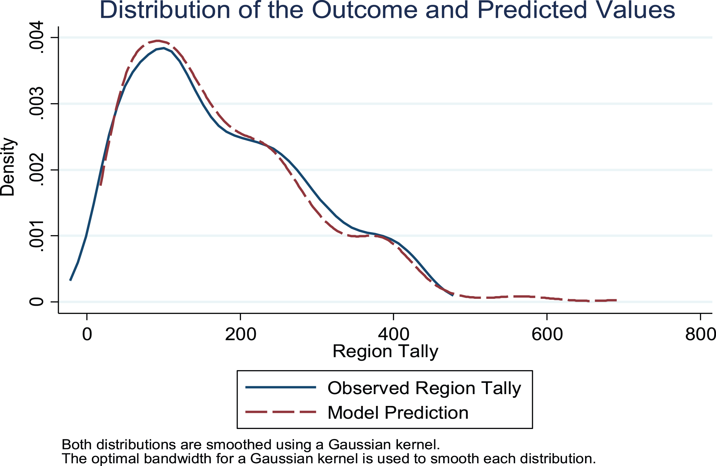
When Opposing Teams in Region and Finalists Avg. Opposing Teams in Region are included, as shown in Equation 1b, all five coefficients take the expected sign, but only Player in Region, Opposing Teams in Region and Finalists Avg. Opposing Teams in Region are statistically significant (P < 0.01). Again, in order to interpret these parameter estimates, average marginal effects for each variable are calculated as previously described. Average marginal effects show these coefficients translate to finalists receiving tallies 42.9 points higher in their home regions than in other regions and 4.9 points higher for each game played in-region. Additionally, average marginal effects show finalists receive 1.38 points less in each region for each 10 percentage point share of other finalists from within-region and 3.9 points less per an average one game increase among games played in-region by other finalists. Further note that to the extent that the variables in Equation 1b are correlated with other predictors of Region Tally that are omitted from Equation 1b, such as National TV, the coefficient estimates from Equation 1b may be biased such that they may not be able to provide a direct causal interpretation. Figure 3 shows the distribution of the outcome variable, Region Tally, and the predicted values from Equation 1b, and highlights how well the model does at matching the observed values (McFadden’s Pseudo R2 = 0.23).
Fig.3
Distributions of outcome and predicted values. Notes: Data from all years 1990–2016 were used to estimate each distribution. The graph shows the distribution of the observed region tally and the predicted values from estimation of Equation 1b, which includes ‘player in region,’ ‘fraction other finalists in region,’ the interaction term between the two variables, ‘fraction other finalists in region,’ finalists avg. opposing teams in region,’ and player-year and region fixed effects. Figure 3 shows the model does a good job of predicting the distribution of regional vote tallies.
3.2The role of nationally televised games
Estimation of Equation 1c and the full model shown in Equation 1 is shown in Table 4. Again, statistical significance of each model parameter is tested at the 1%, 5%, and 10% significance levels, and average marginal effects of each variable are calculated in order to better interpret the model. In the more basic specification shown in Equation 1c, each coefficient takes the expected sign, with Player in Region, Fraction Other Finalists in Region, Player in Region * National TV and Fraction Other Finalists in Region * Outside Finalists National TV statistically significant (P < 0.01, P < 0.01, P < 0.01, and P < 0.1, respectively). In the full specification shown in Equation 1 each coefficient once again takes the expected sign, though only Player in Region, Player in Region * National TV,Opposing Teams in Region, Finalists Avg. Opposing Teams in Region, and Opposing Teams in Region * National TV are statistically significant (P < 0.01, P < 0.1, P < 0.01, P < 0.05, and P < 0.1, respectively). Average marginal effects from the model result in a one game increase in National TV decreasing the vote tally by 1.2 points per game in a finalist’s home region and increasing the vote tally for a finalist by 2.1 points per game in regions outside his home region, all else equal.
Table 4
Unconditional fixed-effects negative binomial (NB2) model coefficients including national television schedule interactions
| Coefficient estimate | Standard error | p-Value | Coefficient estimate | Standard error | p-Value | |
|---|---|---|---|---|---|---|
| Player in Region | 0.650 | 0.085 | <0.001 | 0.382 | 0.091 | <0.001 |
| Fraction Other Finalists in Region | –0.456 | 0.166 | 0.006 | –0.141 | 0.148 | 0.341 |
| Player in Region*Fraction Other Finalists in Region | –0.111 | 0.164 | 0.497 | –0.125 | 0.169 | 0.460 |
| Player in Region*National TV | –0.031 | 0.009 | <0.001 | –0.018 | 0.011 | 0.096 |
| Fraction Other Finalists in Region*Outside Finalists National TV | 0.031 | 0.016 | 0.052 | 0.009 | 0.015 | 0.543 |
| Opposing Teams in Region | 0.046 | 0.013 | <0.001 | |||
| Finalists Avg. Opposing Teams in Region | –0.049 | 0.024 | 0.040 | |||
| Opposing Teams in Region*National TV | –0.003 | 0.001 | 0.083 | |||
| Finalists Opposing Teams in Region*Other Finalists National TV | 0.003 | 0.002 | 0.119 | |||
| alpha | 0.022 | 0.007 | <0.001 | 0.018 | 0.005 | <0.001 |
Notes: Data from all years 1990–2016 were used to estimate the model. Each coefficient can be interpreted as the expected change in the difference in logs of expected ‘region tally’ associated with a unit increase in the corresponding predictor variable. Large attenuation occurs in coefficient estimates on ‘player in region,’ ‘fraction other finalists in region,’ and interactions with ‘national TV’ when ‘opposing teams in region,’ ‘finalists avg. opposing teams in region,’ and the interaction of each with ‘national TV’ are added to the model due to positive correlations with added variables. The p-value of alpha is calculated from the likelihood ratio chi-square test that alpha equals zero. Both models also include player-year and region fixed-effects and a constant, which are not shown in the table for the sake of brevity.
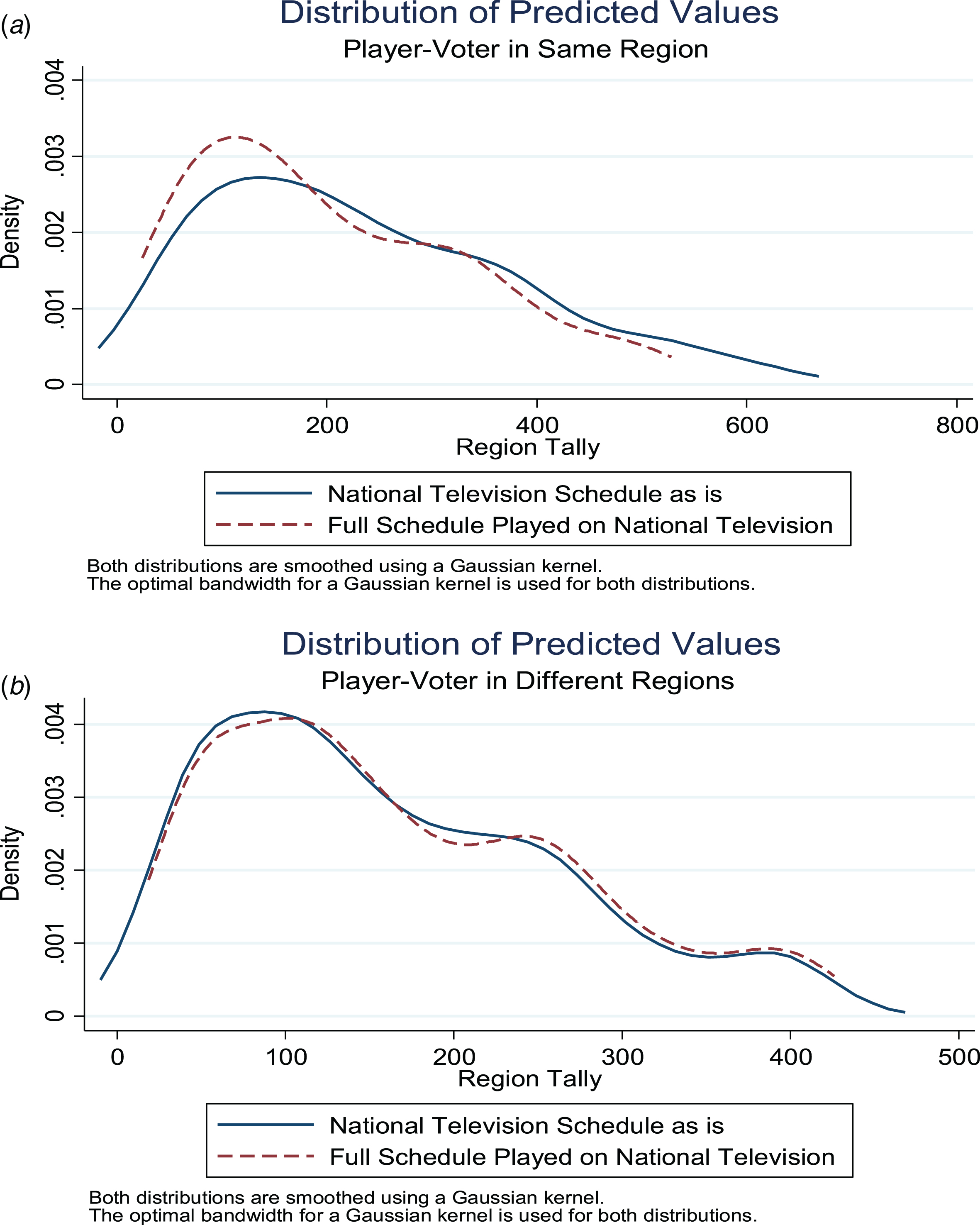
As shown in Fig. 4, under the counterfactual distribution that each team plays a full 13-game schedule on national television, the distribution of predicted values when the player and voter are in the same region shifts substantively to the left and the distribution of predicted values when the player and voter are in different regions shifts ever so slightly to the right. The overall result of increased national television coverage is a decrease in same-region bias.
Fig.4
Shifts in the distribution of predicted values when all games are played on national television. Notes: Data from all years 1990–2016 were used to estimate the model. The full model in Equation 1 is first estimated using the observed value of all variables and then re-estimated under the counterfactual assumption that all finalists play a 13-game national television schedule. The top graph shows the change in the distribution of predicted values when the player and voters are in the same regions and the bottom graph shows the change in the distribution of predicted values when the player and voters are in different regions.
It is worth noting that some variables in the model may be highly correlated. One example may be the interaction terms Fraction Other Finalists in Region * Outside Finalists National TV and Finalists Avg. Opposing Teams in Region * Other Finalists National TV. Because these terms may be highly correlated estimates of their coefficients and standard errors may be very sensitive to the inclusion of the other in the model. This may result in imprecise coefficient estimates, which may in turn lead to a determination that each interaction term is not a statistical significant predictor of regional vote tallies when in fact one or both may be.
3.3Sensitivity analysis
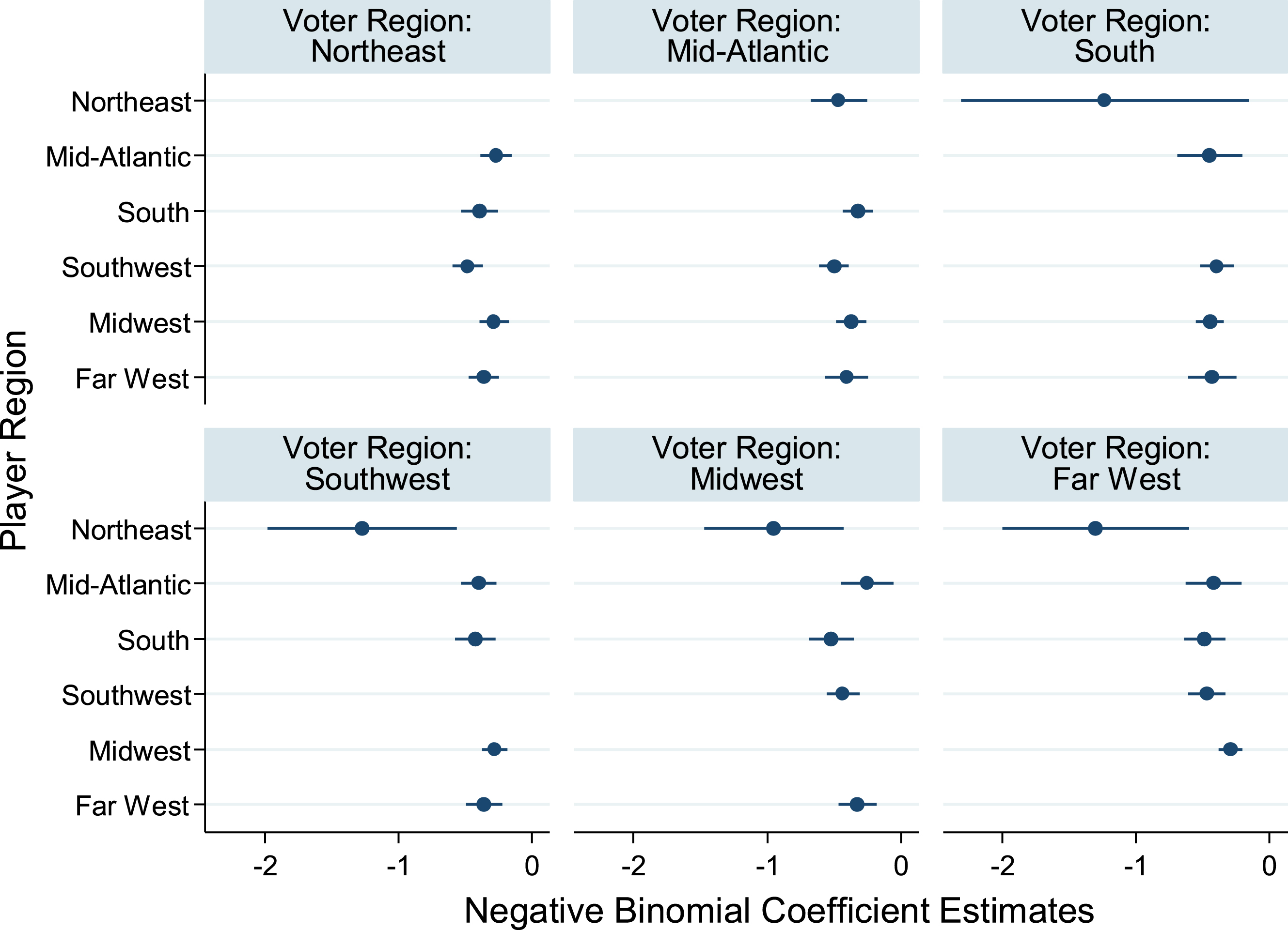
A sensitivity analysis of Equation 1a is estimated replacing the variable Player in Region and the set of voter-region indicator variables with the single set of player- and voter-region specific indicator variables Player Voter Regions r j = PVRrji,j,t, r ∈ {Northeast, Mid-Atlantic, South, Southwest, Midwest, Far West}, with respective coefficients
(2)
When all terms of Player Voter Regions r j where r = j are omitted, each included
Fig.5
Cross-region negative binomial regression estimates. Notes: Data from all years 1990–2016 were used to estimate the model, which is a sensitivity analysis of Equation 1a estimated replacing ‘player in region’ and voter-region indicator variables with a set of indicator variables specific to each combination of player-region and voter-region; indicator variables where player-region and voter-region are the same are excluded. Each dot represents the negative binomial coefficient and each bar represents the 95% confidence interval around the coefficient estimate. Each coefficient represents the difference between vote tallies for players in the region corresponding to the coefficient and players sharing the same region as the voters. Statistically significant differences (P < 0.05) exist in each of the following regions between players from regions in parenthesis: Northeast (Mid-Atlantic, Southwest), (Midwest, Southwest); Mid-Atlantic (South, Southwest); Southwest (Midwest, South), (Northeast, all other regions); Midwest (Mid-Atlantic, Northeast), (Far West, Northeast), (Far West, South); Far West (Midwest, South), (Midwest, Southwest), (Northeast, all other regions). Because each coefficient is tested against the other four coefficients in the voter region, another set of tests were conducted using the Bonferroni correction with four comparisons at the 5% significance level. All aforementioned differences remain statistically significant (P < 0.05) except in the Far West region between players from the Northeast and South and players from the Northeast and Southwest.
An additional sensitivity analysis fully interacting Player Voter Regions r j with Fraction Other Finalists in Region s = FOFiRsi′,t, the fraction of other finalists from region s (for each region s), is estimated that also includes region-specific estimates of coefficients on Opposing Teams in Region and Finalists Avg. Opposing Teams in Region. This results in the following equation:
(3)
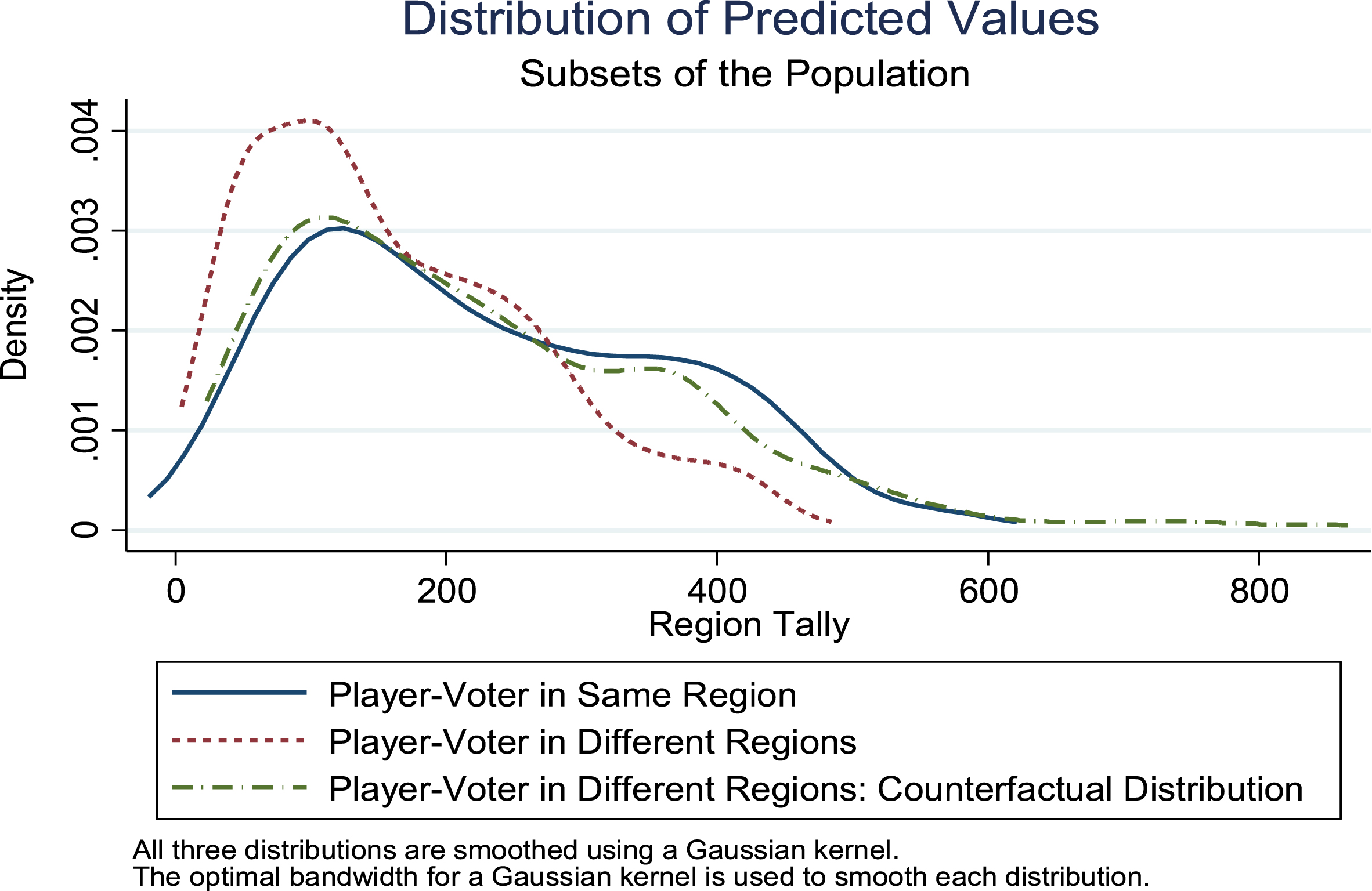
This sensitivity analysis is used to compare the distributions of expected regional vote tallies when the player and voters are from the same region and from different regions, and to estimate the counterfactual distribution when the player and voters are from different regions. This counterfactual distribution is estimated by changing the player region r to take the value j and setting Opposing Teams in Region = E (Opposing Teams in Region |r = j) for observations where r ≠ j. The distribution of predicted values when the player and voter are in different regions is far to the left of the distribution when the player and voter are in the same region, but estimation of the counterfactual shifts this distribution far to the right to more closely mirror the distribution when the player and voter are in the same region. This sensitivity analysis provides further evidence of same-region bias and shows that estimates of same-region bias shown in previous subsections was not an artifact of more simplified specifications of the model. These distributions are presented in Fig. 6.
Fig.6
Distributions of outcome and predicted values for subsets of the population. Notes: Data from all years 1990–2016 were used to estimate the distributions, which come from a sensitivity analysis of Equation 1b that fully-interacts a set of indicator variables specific to each combination of player-region and voter-region with the fraction of other finalists that share the region with the player in question for each region and also includes region-specific estimates of coefficients on ‘opposing teams in region’ and ‘finalists avg. opposing teams in region.’ The graph shows distributions of predicted values when the player and voter are in the same region, when the player and voter are in different regions, and the counterfactual distribution when the player and voter are in different regions. This counterfactual distribution is estimated by changing the player region to take the value of the voter region and setting ‘opposing teams in region’ to the expected value among finalists in the same region as the voter for finalists from a different region than the voters. The distribution of predicted values when the player and voter are in different regions is far to the left of the distribution when the player and voter are in the same region, but estimation of the counterfactual shifts this distribution far to the right to more closely mirror the distribution when the player and voter are in the same region.
While not shown for the sake of brevity, a sensitivity analysis of Equation 1a is estimated where Player in Region is interacted with region indicator variables γ to determine the regions where same-region bias is most prevalent. This results in the following equation:
(4)
The largest same-region bias is found in the Northeast, followed by the South, Southwest, and Far West, and finally the Mid-Atlantic and Midwest, though only differences between the Northeast and other regions are statistically significant at any relevant significance levels.
4Conclusion
While there has been wide-spread speculation on the existence and nature of regional bias in Heisman voting, before now there has not been a peer-reviewed academic study verifying the existence, nor commenting on the nature, of such bias. This has led to a number of misconceptions, such as a wide-ranging belief that finalists from the Far West region are treated adversely by voters in other regions as compared to the rest of the field. However, the majority of previous conclusions are corroborated and augmented with further inferences.
The analysis presented in this article explores the nature of such bias in Heisman voting with an unconditional fixed-effects negative binomial regression (NB2) model that includes indicator variables to represent player-year fixed effects using regional data on Heisman finalists from 1990–2016. Results show Heisman finalists do receive higher vote tallies in their home regions on average. In addition, the results establish that regional Heisman vote tallies are decreasing in the fraction of other finalists based within-region. Furthermore, evidence reveals that finalists receive higher regional vote tallies for each additional game played against a team located within-region and lower regional vote tallies for each additional game played against a team located within-region by other finalists. The analysis is augmented by showing that the increase in national television coverage of college football games has been accompanied by a decrease in the prevalence of regional bias. However, there is no evidence that finalists from the Far West receive lower vote tallies in other regions compared to other out-of-region finalists; to the contrary, evidence suggests finalists from the Northeast, South, and Southwest are more likely to be treated adversely in other regions.
Future analyses might seek to further clarify the results presented here by explaining why voters tend to vote for players based in their region. For instance, do voters tend to vote for in-region players because the information they receive is biased due to familiarity with local candidates, or are other explanations such as regional pride or personal emotions at play? Alternatively, one might seek to include other potential drivers of regional preferences not observed here, such as heterogeneous preferences among voters across regions or voter commonality with Heisman candidates (perhaps along racial or ethnic lines). Additionally, other recent changes have occurred that provide Heisman voters with more information, such as increased access to the internet and further reliance on objective statistical metrics to evaluate performance. Further studies might seek to analyze the extent to which these changes may explain some of the reduction in regional bias attributed to the expansion of national television schedules in this analysis.
References
1 | Allison P. & Waterman R. , Fixed-effects negative binomial regression models. In Stolzenberg R. (Ed.), Sociological Methodology. Oxford: Basil Blackwell. |
2 | Allison P. (2009) , Fixed Effects Regression Models. Thousand Oaks, CA: Sage. |
3 | Alzo L. , & Oxenreiter A. , (2007) , Sports memories of Western Pennsylvania: Images of sports. Charleston, SC: Arcadia. |
4 | Burbank M. (1995) , How do contextual effects work? Developing a theoretical model. In Eagles M. (Ed.), Spatial and contextual models in political research. London: Taylor and Francis. |
5 | Cox K. (1969) , The voting decision in a spatial context. In Board C. , Chorley R. , Haggett P. , & Stoddart D. (Eds.), Progress in geography 1. London: Edward Arnold. |
6 | Curtice J. , & Steed M. , Electoral choice and the production of government. The changing operation of the electoral system in the United Kingdom since 1955, British Journal of Political Science, 12: (3), 249–298. |
7 | Chisolm K. (2003) , West coast bias? Stiff Arm Trophy. Retrieved from http://archive.stiffarmtrophy.com/2003/10/ west coast bias.html . |
8 | Donchess J. (2014) , Heisman voting bias. D Ratings. Retrieved from http://www.dratings.com/heisman-voting-bias/ . |
9 | Drape J. (2001) , Sentiment could sway Heisman: College football sentiment could sway Heisman vote, New York Times. |
10 | Fitton M. , (1973) Neighbourhood and voting: A sociometric explanation, British Journal of Political Science, 3: (4), 445–472. |
11 | Haptonstall C. (2005) , Measuring the effectiveness of mediated and non-mediated communication among Heisman trophy voters (Doctoral dissertation). Florida State University, Tallahassee, Florida. |
12 | Heard D. (2013) , Predicting Heisman trophy voting: A Bayesian analysis. Proceedings of the 2013 New England Symposium on Statistics in Sports. Harvard University, Cambridge, Massachusetts. |
13 | Heisman J. , & Schlabach M. (2012) , Heisman: The man behind the trophy. New York: Howard Books. |
14 | Heisman . (2014) , Heisman trophy balloting. Heisman. Retrieved from http://heisman.com/sports/2014/9/15/GEN_ 0915140346.aspx . |
15 | Heisman . (2017) , Heisman winners. Heisman. Retrieved from http://heisman.com/roster.aspx?path=football . |
16 | Huston C. (2016) , Heisman balloting: How itworks. Retrieved from http://heisman.com/news/2016/11/17/Heisman_ Winners_1117162029.aspx?path=heisman_ winners. |
17 | Horne L. (2013) , Tracing the evolution of the Heisman trophy. Bleacher Report. Retrieved from http://bleacherreport. com/articles/1609504-tracing-the-evolution-of-the-heisman-trophy-award. |
18 | Jacobson S. (1971) , Ivy League image a drawback to Marinaro in Heisman vote: Heisman bias, Los Angeles Times. |
19 | Johnston R. (1983) , The neighbourhood effect won’t go away: Observations on the electoral geography of England in the light of Dunleavy's critique, Geoforum, 14: (2), 161–168. |
20 | Johnston R. , (1986) The neighbourhood effect revisted: Spatial science or political regionalism?, Environment and Planning 4: (1), 41–55. |
21 | Knox L. , & Grossman H. , (2015) Derrick Henry, Heisman finalists will feel the regional love.Retrieved from, ABC News. 2015 http://abcnews.go.com/Sports/derrick-henry-heisman-finalists-feel-regional-love/story?id=35706468 . |
22 | McCartney C. The Heisman trophy: The story of an American icon and its winners (2016) . New York: Skyhorse Publishing. |
23 | The Oklahoman. (2003) , Regional bias a Heisman concern. The Oklahoman. |
24 | Outside the Sidelines. (2007) , Will Alabama ever have a Heisman trophy winner? Roll ’Bama Roll Blog. Retrieved from http://www.rollbamaroll.com/2007/8/28/15938/0833 . |
25 | Pattie C. , & Johnston R. (2000) , “People who talk together vote together”: An exploration of the neighbourhood effect in Great Britain, Annals of the Association of American Geographers, 90: (1), 41–66. |
26 | Pennington B. (2010) , Reggie Bush, ineligible for ’05, returns Heisman. New York Times. |
27 | Spurrier S. (2012) . Review of J. Heisman & M. Schlabach, Heisman: The man behind the trophy. Retrieved from http://www.amazon.com/Heisman-The-Man-Behind-Trophy/dp/1451682948 . |
28 | Taylor P. & Johnston R. (1979) . Geography of elections. New York: Holmes & Meier. |
29 | Weinreb M. (2016) , Catch him if you can. The Ringer. Retrieved from https://theringer.com/christian-mccaffrey-stanford-cardinal-heisman-trophy-bias-8a13066687ac . |
30 | Wilner J. (2009) , Toby Gerhart and the Heisman trophy: Analyzing the voting blocs. College Hotline Blog. Retrieved from http://blogs.mercurynews.com/collegesports/2009/12/11/toby-gerhart-and-the-heisman-trophy-analyzing-the-voting-blocs/.blocs/ . |


