
A multi-season machine learning approach to examine the training load and injury relationship in professional soccer
Abstract
OBJECTIVES:
The purpose of this study was to use machine learning to examine the relationship between training load and soccer injury with a multi-season dataset from one English Premier League club.
METHODS:
Participants were 35 male professional soccer players (aged 25.79±3.75 years, range 18–37 years; height 1.80±0.07 m, range 1.63–1.95 m; weight 80.70±6.78 kg, range 66.03–93.70 kg), with data collected from the 2014–2015 season until the 2018–2019 season. A total of 106 training loads variables (40 GPS data, 6 personal information, 14 physical data, 4 psychological data and 14 ACWR, 14 MSWR and 14 EWMA data) were examined in relation to 133 non-contact injuries, with a high imbalance ratio of 0.013.
RESULTS:
XGBoost and Artificial Neural Network were implemented to train the machine learning models using four and a half seasons’ data, with the developed models subsequently tested on the following half season’s data. During the first four and a half seasons, there were 341 injuries; during the next half season there were 37 injuries. To interpret and visualize the output of each model and the contribution of each feature (i.e., training load) towards the model, we used the Shapley Additive Explanations (SHAP) approach. Of 37 injuries, XGBoost correctly predicted 26 injuries, with recall and precision of 73% and 10% respectively. Artificial Neural Network correctly predicted 28 injuries, with recall and precision of 77% and 13% respectively. In the model using Artificial Neural Network (the relatively more accurate model), last injury area and weight appeared to be the most important features contributing to the prediction of injury.
CONCLUSIONS:
This was the first study of its kind to use Artificial Neural Network and a multi-season dataset for injury prediction. Our results demonstrate the potential to predict injuries with high recall, thereby identifying most of the injury cases, albeit, due to high class imbalance, precision suffered. This approach to using machine learning provides potentially valuable insights for soccer organizations and practitioners when monitoring load injuries.
1Introduction
Monitoring the load placed on athletes in training and competition is a current “hot topic” (Kalkhoven et al., 2021) in sport science, with professional sports teams investing substantial resources to this end (Bourdon et al., 2017). Load monitoring is essential for determining adaptation to training programs, assessing fatigue and recovery, and minimizing the risk of injury and illness (Kalkhoven et al., 2021; Halson, 2014). As the most popular global sport, with 200,000 professional and 240 million amateur players, and with injury incidence higher than any other sport (Rahnama, 2011; Owoeye et al., 2020; Jones et al., 2019), soccer has become a key focus for research into load monitoring and injury. Soccer injuries can lead to extended periods of absence from matches, with associated impacts on team performance, as well as financial implications (Rahnama, 2011; Owoeye et al., 2020; Jones et al., 2019; Ibrahimović et al., 2021). Indeed, from 2012–2013 through to the 2016–2017 season, injuries cost English Premier League soccer clubs approximately £45 million per season (Eliakim et al., 2020). In attempting to better understand the relationship between training load and soccer injury, recent research has begun to draw on techniques from machine learning (for a review, see Majumdar et al., 2022). In the present study, we employed a multi-dimensional and multi-season interpretable machine learning approach to examine the relationship between training load and soccer injury using data from one English Premier League club.
The timeliness of using machine learning for sports injury prediction is highlighted by recent reviews (Van Eetvelde et al., 2021; Rossi et al., 2021). Machine learning approaches can help expand the focus from more simplified models of the injury process—such as when using the Acute Chronic Workload Ratio (ACWR) (Hulin et al., 2013), the most popular and well-researched model of the injury process—to create a better understanding of the relative influence of various (physical and psychological) aspects of training load on injury risk. The original research into the ACWR (Hulin et al., 2013) in the sport of cricket suggested an optimal ACWR range of between 0.85 and 1.5, with ACWR values exceeding 1.5 leading to a 2–4 times greater injury risk. But there have been recent methodological and theoretical criticisms of ACWR (e.g., see Impellizzeri et al., 2021). Further, although tests of the ACWR with data from the English Premier League (Bowen et al., 2019) have shown that if the ACWR exceeds a value of 2 when chronic load is low, there is 5–7 times greater risk of injury, other work within Italian professional soccer (Rossi et al., 2018) has not observed any training sessions with ACWR values exceeding 2, finding that the highest injury risks occur when the ACWR is less than 1. These sorts of concerns and equivocal results have led to recent machine learning research examining soccer injury with a greater number or explanatory load variables (Rossi et al., 2018; Vallance et al., 2020; Naglah et al., 2018; Lopez-Valenciano et al., 2018; Ayala et al., 2019; Rommers et al., 2020; Oliver et al., 2020; Venturelli et al., 2011; Kampakis, 2016). The above notwithstanding, however, there are a number of limitations in this research that have been noted (Majumdar et al., 2022). These include, though are not limited to, a need for (a) greater clarity with regard to the reported evaluation metrics (e.g., recall and precision), and whether they are “per-class” of injury or “averaged” across injury and non-injury data; (b) greater detail regarding the various pre-processing techniques employed (e.g., in relation to any missing values, different data imputation techniques required, balancing, and clarity regarding all types of demographic data, and internal and external load variables); and (c) studies over more than one season, wherein models are tested and refined on subsequent seasons’ data, with their inherent changes in players, coaches, training, and matches.
In the present study we addressed each of these limitations, examining the relationship between training load and soccer injury with a multi-season dataset from one English Premier League club. The latter point is important, because previous research has, with the exception of the work of Rossi and colleagues (2018), tended to focus on developing models with just one season’s data, using cross-validation and train-validation split, leaving questions as to how accurate such models would be in predicting “unseen” data (such as from a subsequent season). Specifically, then, our novel approach was to train models on data collected across four and a half soccer seasons, and then to test those models on the next unseen half season’s data. Alongside addressing the known limitations of previous papers, we also sought to examine multiple forms of data (e.g., Global Positioning System data, physical data, psychological data, and demographic data)—something only Vallance et al. (2020) had previously reported.
To provide the best opportunity to then unearth insights with our training load input data and injury output data, we drew upon state-of-the-art processes from machine learning (such as using the XGBoost algorithm: Chen and Guestrin, 2016), but also drew upon deep learning, wherein the employed algorithms are inspired by the structure and functions of biological neural networks—often called Artificial Neural Networks (or ANNs) (Mehlig, 2019). Finally, we should note another criticism of previous papers examining load monitoring and soccer injury—the lack of clarity with regard to the key variables underpinning the machine learning models developed. This is important, because if machine learning is to become a key part of a practitioner’s toolkit in understanding injury risk, machine learning models need to provide clarity with regard to the causes of (or key risks for) injury—i.e., the importance of “interpretability” (Belle and Papantonis, 2020). In this context, white-box models use algorithms (e.g., linear regression, logistic regression, k-nearest neighbors, decision tree) that are interpretable, presenting a clear mapping from inputs to outputs, clarifying how analysis decisions are made—and potentially aiding practitioners and clinicians in deriving applied implications from such research (Loyola-Gonzalez, 2019). On the other hand, black-box models use algorithms (e.g., ensemble methods, random forest, artificial neural networks, support vector machine) that are not easily interpretable, but may be more powerful. In the latter examples, the mapping from inputs to outputs is opaque, but additional post-hoc methods can then be used to interpret and understand the results (Loyola-Gonzalez, 2019). In the present study, we employed black-box methods, and thus to aid interpretability, we employed the Shapley Additive exPlanations (SHAP) approach (Lundberg and Lee, 2017)—an explainability framework based on game theory, which can be used to unpick the key predictors of machine learning models by computing the contribution of each feature to prediction.
Overall, then, in the first study of its type, we report a novel approach which can address gaps in existing research and produce a practical solution for soccer injury prediction. Through comprehensive analysis of a unique multi-season dataset of Elite Premier League soccer players, we aimed to develop a multi-dimensional predictive machine learning model to assess injury risk among players in the following seven days.
2Materials and methods
2.1Data collection and feature creation
Participants were 35 male professional soccer players (aged 25.79±3.75 years, range 18–37 years; height 1.80±0.07 m, range 1.63–1.95 m; weight 80.70±6.78 kg, range 66.03–93.70 kg) from one English Premier League club, with data collected from the 2014–2015 season until the 2018–2019 season. Players’ positions were recorded as follows: eight full-backs, nine center-backs, seven central mid-fielders, eight wing-forwards, and three strikers. Data were provided to the research team by the club’s first team sports science department, having been collected as part of the club’s day-to-day data collection processes, and with all permissions in place. The dataset contained 343 injury data points, of which our focus was the 133 non-contact injuries. Of these 133 non-contact injuries, there were 43 thigh injuries, 29 knee injuries, 24 hip injuries, 19 ankle injuries, and 18 ‘lower leg’ injuries. Across injuries, eight players were injured once, nine players were injured two times, four players were injured three times, two players were injured four times, four players were injured five times, two players were injured six times, four players were injured seven times, one player was injured 11 times, and one player was injured 16 times. Overall, there were 11 injuries recorded in the 2014–2015 season, six in the 2015–2016 season (the club’s first in the English Premier League), 28 in the 2016–2017 season, 41 in the 2017–2018 season, and 47 in the 2018–2019 season.
The available ‘load’ data included Global Positioning System (termed GPS) data, physical (e.g., various skinfold measurements, bodyfat percentage) data, psychological (e.g., RPE) data, and demographic information. Feature selection first focused on removing features with more than 60% missing values. Please note, when players missed training sessions, their absence of training load data is not noted in the dataset, and is thus not treated as missing data. Subsequently, different missing values imputation methods were used across the features. We also created two additional features within the dataset: “last injury area” and “days since last injury”. In the Appendix, Table 1 lists all training load variables considered as input features in the present study, along with their description, source, method of collection, frequency of data collection (e.g., GPS and psychological data are collected daily; physical data are collected every two weeks), and missing values imputation techniques.
Table 1
Training load variables, variable descriptions, missing value imputation techniques, method of data collection, and data collection frequency
| Variable Name | Variable Description | Missing Value Imputation | Method of data collection | Frequency of data collection |
| GPS measures/External Load | ||||
| Total Duration | Total time in minutes an athlete is in activity | knn | Time taken from activity on GPS device | Every pitch session and game |
| Total Distance (m)* (TDM) | Distance in meters covered during the activity | knn | GPS device | Every pitch session and game |
| Meterage Per Minute* (MPM) | Distance in meters covered during the activity per minute | knn | GPS device | Every pitch session and game |
| Sprint Efforts* (SE) | Number of efforts above 7 m/s | knn | GPS device | Every pitch session and game |
| Sprint Distance (m) | Distance in meters covered above 7 m/s | knn | GPS device | Every pitch session and game |
| High Speed Distance (m)* (HSD) | Distance in meters covered above 5.5 m/s | knn | GPS device | Every pitch session and game |
| High Speed Distance Per Minute (m/min) (m) | Distance in meters covered above 5.5 m/s per minute of activity | knn | GPS device | Every pitch session and game |
| Maximum Velocity (m/s)* (MV) | Maximum velocity reached in activity | knn | GPS device | Every pitch session and game |
| Velocity Band 7 Total Effort Count | Number of efforts above 90% of players maximum velocity | knn | GPS device | Every pitch session and game |
| Velocity Band 7 Total Distance (m) | Distance in meters covered above 90% of players maximum velocity | knn | GPS device | Every pitch session and game |
| Total Player Load* (TPL) | Sum of the accelerations across all axes of the internal tri-axial accelerometer during movement. It considers instantaneous rate of change of acceleration and divides it by a scaling factor (divided by 100). | knn | GPS device | Every pitch session and game |
| Accels* (ACC) | Number of accelerations above 0.5 m/s2 | knn | GPS device | Every pitch session and game |
| Decels* (DCC) | Number of decelerations above –0.5 m/s2 | knn | GPS device | Every pitch session and game |
| Perceived Exertion* (PE) | The Borg Rating of Perceived Exertion (RPE) using Borg CR10 Scale | knn | Questionnaire | Every pitch session and game |
| Workload* (WD) | Perceived Exertion × Total Duration | knn | Calculation of Total Duration x RPE | Every pitch session and game |
| Meta Energy (KJ/kg) * (ME) | Estimated energy expenditure, based on GPS acceleration | knn | GPS device | Every pitch session and game |
| Velocity Work/Rest Ratio | Time working divided by Time resting where work and rest are defined by velocity thresholds | knn | GPS device | Every pitch session and game |
| Work/Rest Ratio | The amount of time spent above the work velocity threshold divided by the amount of time spent below the rest velocity threshold | knn | GPS device | Every pitch session and game |
| Relative Intensity | (High Speed Distance (m)/Total Distance (m)) * 100 | knn | GPS device | Every pitch session and game |
| Mean Heart Rate | Average heart rate (beats per minute) in activity | knn | GPS device | Every pitch session and game |
| Maximum Heart Rate | Maximum heart rate (beats per minute) in activity | knn | GPS device | Every pitch session and game |
| Player Load Per Minute | Average Player Load accumulated per minute of activity | knn | GPS device | Every pitch session and game |
| Player Load (1D Fwd) | Player Load accumulated in the sagittal plane | knn | GPS device | Every pitch session and game |
| Player Load (1D Side) | Player Load accumulated in the frontal plane | knn | GPS device | Every pitch session and game |
| Player Load (1D Up) | Player Load accumulated in the sagittal plane | knn | GPS device | Every pitch session and game |
| Player Load (2D) | Player Load accumulated in the frontal and sagittal planes | knn | GPS device | Every pitch session and game |
| RHIE Total Bouts | The total occurrences of Repeated High Intensity Effort (RHIE) events | knn | GPS device | Every pitch session and game |
| RHIE Effort Duration –Mean | The average duration of a RHIE event | knn | GPS device | Every pitch session and game |
| RHIE Effort Duration –Min | The shortest duration of a RHIE event | knn | GPS device | Every pitch session and game |
| RHIE Effort Duration –Max | The longest duration of a RHIE event | knn | GPS device | Every pitch session and game |
| RHIE Bout Recovery –Mean | The average amount of time between RHIE events | knn | GPS device | Every pitch session and game |
| RHIE Bout Recovery –Min | The shortest time between RHIE events | knn | GPS device | Every pitch session and game |
| RHIE Bout Recovery –Max | The longest amount of time between RHIE events | knn | GPS device | Every pitch session and game |
| IMA Jump Count Low Band | The total number of jumps registered 0–20 cm | knn | GPS device | Every pitch session and game |
| IMA Jump Count Med Band | The total number of jumps registered 20–40 cm | knn | GPS device | Every pitch session and game |
| IMA Jump Count High Band | The total number of jumps registered >40 cm | knn | GPS device | Every pitch session and game |
| HMLD* | Distance in meters covered by a player where his/her Metabolic Power is >25.5 W/kg | knn | GPS device | Every pitch session and game |
| HML Distance Per Minute (m/min) (m) | Distance in meters covered by a player where his/her Metabolic Power is >25.5 W/kg per minute | knn | GPS device | Every pitch session and game |
| Explosive Efforts* (EE) | IMA Accel High + IMA Decel High + IMA CoD Left High + IMA CoD Right High + IMA Accel Medium + IMA Decel Medium + IMA CoD Left Medium + IMA CoD Right Medium | knn | GPS device | Every pitch session and game |
| Explosive Efforts per Min* (EEM) | EE/minute | knn | Calculation | Every pitch session and game |
| Personal Information | ||||
| Age | Age of player | |||
| BMI | Body Mass Index; ratio between weight (in kg) and the square of height (in meters) | None | Calculation | |
| Height | Player’s height in centimetres | None | Measurement from Sadiometer | Pre-season |
| Weight | Players weight in kilograms | Linear Interpolation | Measurement from Secca Scales | Fortnightly |
| Last Injury Area | Last injury area | None | ||
| Days since last injury | None | |||
| Internal Load –Physical data | ||||
| TRICEP | Triceps’ skinfold measurement | Linear Interpolation | Skinfold measurement taken with Harpenden Callipers | Fortnightly |
| SUBSCAP | Subscapular skinfold measurement | Linear Interpolation | Skinfold measurement taken with Harpenden Callipers | Fortnightly |
| BICEP | Bicep skinfold measurement | Linear Interpolation | Skinfold measurement taken with Harpenden Callipers | Fortnightly |
| ILIAC | Iliac Crest skinfold measurement | Linear Interpolation | Skinfold measurement taken with Harpenden Callipers | Fortnightly |
| SUPRA | Supraspinal skinfold measurement | Linear Interpolation | Skinfold measurement taken with Harpenden Callipers | Fortnightly |
| ABDOM | Abdominal skinfold measurement | Linear Interpolation | Skinfold measurement taken with Harpenden Callipers | Fortnightly |
| THIGH | Thigh skinfold measurement | Linear Interpolation | Skinfold measurement taken with Harpenden Callipers | Fortnightly |
| CALF | Calf skinfold measurement | Linear Interpolation | Skinfold measurement taken with Harpenden Callipers | Fortnightly |
| Skinfolds | Sum of 8 site skinfold measurements | Linear Interpolation | Calculation | Fortnightly |
| % Bodyfat (Yuhasz). | (0.1051 × sum of triceps, subscapular, supraspinal, abdominal, thigh, calf) +2.585 | Linear Interpolation | Calculation | Fortnightly |
| % Bodyfat (Jackson) | (0.29288 × sum of skinfolds) –(0.0005 × square of the sum of skinfolds) + (0.15845 × age) –5.76377 | Linear Interpolation | Calculation | Fortnightly |
| Fat Mass | (Weight/100)* % Bodyfat (Jackson) | Linear Interpolation | Calculation | Fortnightly |
| Lean Mass | Weight –Fat Mass | Linear Interpolation | Calculation | Fortnightly |
| Relative Lean Mass | Lean Mass/Weight | Linear Interpolation | Calculation | Fortnightly |
| Internal Load –Psychological data | ||||
| Sleep | Previous night’s sleep quality | Forward fill and back fill | Questionnaire | Every training day |
| Fatigue | Fatigue level | Forward fill and back fill | Questionnaire | Every training day |
| Ext. Stress | Stress level | Forward fill and back fill | Questionnaire | Every training day |
| Soreness | Muscle Soreness | Forward fill and back fill | Questionnaire | Every training day |
| ACWR, MSWR and EWMA | ||||
| ACWR of 14 daily GPS features* | Given a training load feature, the Acute Chronic Workload Ratio (ACWR) is the ratio of acute (i.e., rolling average of training load completed in the past week) to chronic (i.e., rolling average of training load completed in the past 4 weeks) workload. | knn | Calculation | |
| MSWR of 14 daily GPS features* | Monotony of a player. Given a training load feature, MSWR is calculated by taking the ratio of the mean and standard deviation of the values of the training load in the past 1 week/7 days. | knn | Calculation | |
| EWMA of 14 daily GPS features* | Exponential weighted moving average puts greater weight and significance to the most recent training loads (i.e., data points). It follows a decay rule of
| knn | Calculation | |
Note. *These training load variables are used in the calculation of ACWR, MSWR and EWMA.
2.2Dataset construction
We constructed a multi-dimensional load-injury prediction model to forecast whether a player would become injured in the next seven-day window. This seven-day window was chosen to mirror the standard frequency of English Premier League match occurrence—i.e., a match is played approximately every seven days (and generally at the weekend). A similar approach was employed by Vallance et al. (2020). There are generally between three and four training sessions each week, with training loads reaching their peak towards the end of each week.
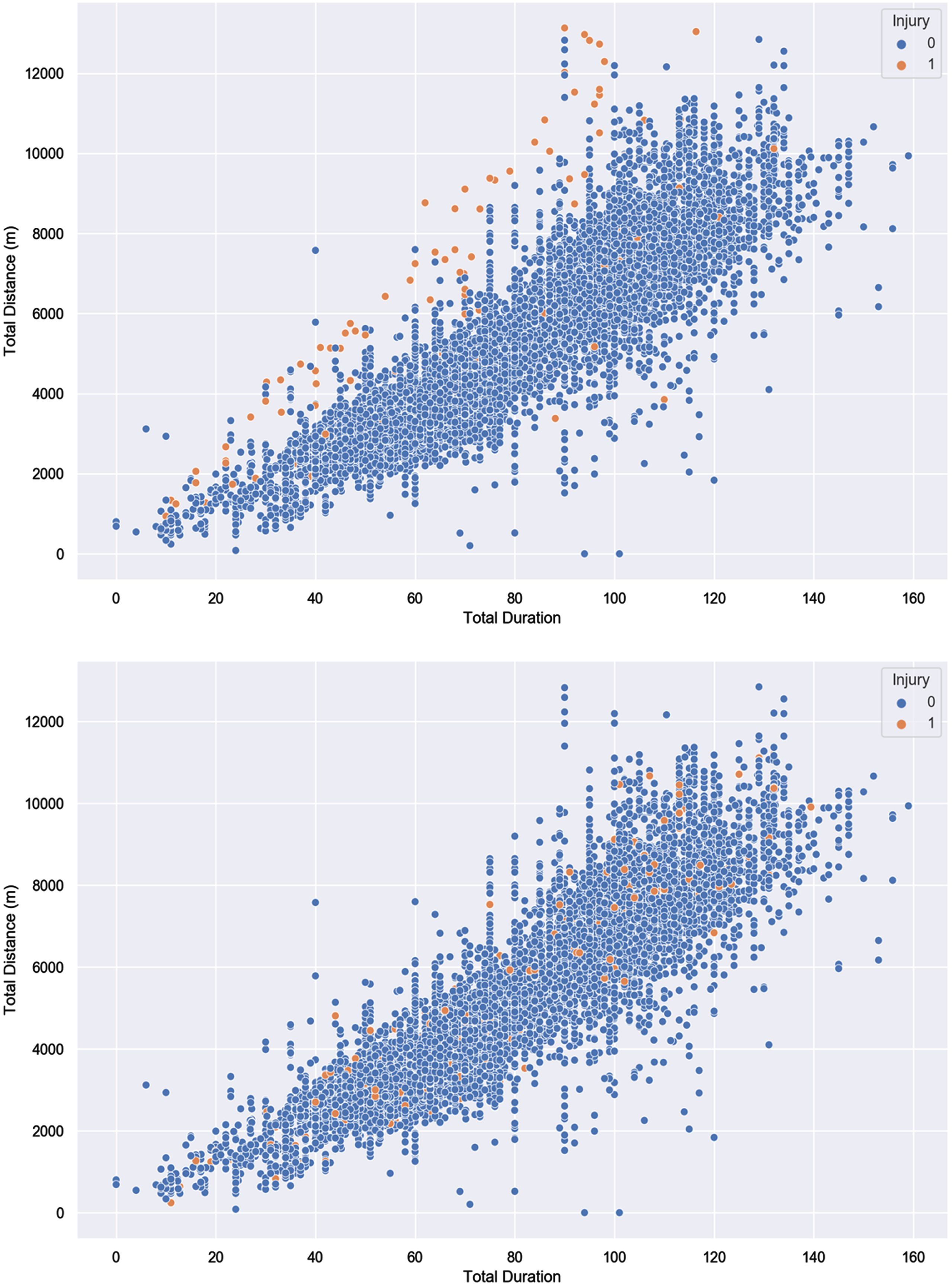
To accomplish the task of constructing an injury prediction model, we initially built a master dataset consisting of 106 training load variables (see Table 1): 40 GPS data variables, six personal information variables, 14 physical data variables, four psychological data variables, 14 ACWR, 14 MSWR, and 14 EWMA data variables (mentioned in Table 1), one injury label (indicating 1 if the player is injured and 0 if not), and 10653 data points (i.e., each data point is a row which describes the training information and personal information for each player). In this master dataset, there were 10,520 non-injury data points and 133 injury data points, indicating a high imbalance ratio of 0.013. Importantly, in this master dataset, the injury label was assigned to the original injuries that happened on the same day (i.e., injuries that were recorded on the day of occurring), but our aim was to predict injuries in the next seven-day window. To achieve the latter focus, we thus assigned the previous data points (i.e., each data point or row that came before the original data points) present in the past seven days of the original injury data point to 1 and removed the original injury data points. The assumption behind removing the original data points is that the injury occurring on a specific day is caused by the training loads of the previous days. As a result, our seven-day injury prediction model is based on a revised dataset containing 10,520 data points, of which there are 10,142 non-injury data points and 378 injury data points, giving an imbalance ratio of 0.037. Figure 1 presents the injury and non-injury distribution in the original and seven-day injury prediction dataset (denoted D) respectively. In the seven-day injury prediction dataset (D) the injury and non-injury data points overlap. Imbalanced and overlapping data classification represent a challenge for traditional machine learning models, which often fail to recognize patterns in such data (Shahee and Ananthakumar, 2021; Kiesow et al., 2021).
Fig. 1
The Relationship Between Graphical Representation of Injury and Non-Injury Distribution in the Original and Seven-Day Injury Prediction Dataset using two training load variables. Note. Top panel: Injury and non-injury distribution in the original dataset. Bottom panel: Injury and non-injury distribution in the seven-day injury prediction dataset. To present the injury and non-injury distribution in both the datasets, total duration and total Distance (m) were used.
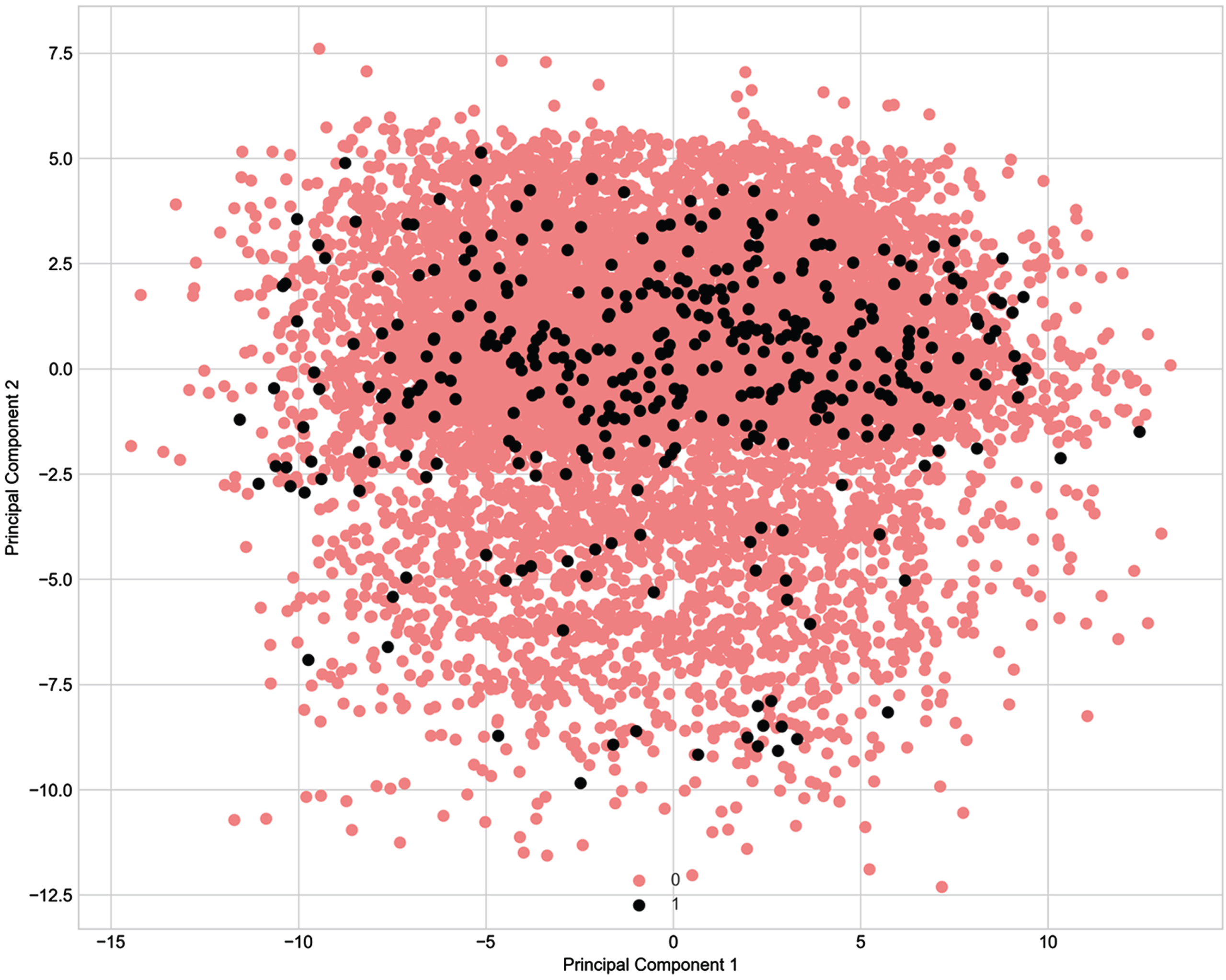
In addition, for a better depiction of the classification problem and how our high-dimensional injury and non-injury datapoints appear in a two-dimensional plane we performed Principal Component Analysis. Figure 2 in the Appendix demonstrates that the injury and non-injury data points are overlapping (Tang et al., 2010; Sáez et al., 2019; Gupta and Gupta, 2018; Shahee and Ananthakumar, 2021; Kiesow et al., 2021). This is illustrated by many instances where similar training programs resulted in different outcomes, which is likely an indication that the features which would clearly separate the two classes are not being currently collected. We should also note that, while calculating ACWR, MSWR and EWMA for each player, we used the training sessions which fell in the past seven days before each training session or match-day. The past seven days may be different from the past seven training sessions as the past seven training sessions might not fall into the past seven days.
Fig. 2
Principal Component Analysis of the Seven-Day Injury Prediction Dataset. Note: Principal component analysis on dataset D (the seven-day injury prediction) with 106 features. Red dots represent non-injury data points; black dots represent injury data points.
2.3Model construction
For model building, validation, and testing, we used the Python programming language. We used various machine learning algorithms—logistic regression, k-nearest neighbors, decision tree, and random forest resulted in poor model performance, failing to predict most of the actual injuries—with XGBoost (Chen and Guestrin, 2016) and Artificial Neural Network (ANN) (Mehlig, 2019) providing the best results. In this paper, we thus focus from this point onwards on the use of and results from the XGBoost and ANN algorithms. We used various pre-processing techniques, such as oversampling the minority data points (i.e., the injury data), feature scaling (i.e., scaling each training load), and setting different hyperparameters.
We first split the entire dataset into two parts—the training data (DTrain), containing the first four and half seasons’ data, and the test data (DTest), containing the remaining half season. DTrain contained 9548 non-injury data points and 341 injury data points and DTest contained 493 non-injury data points and 37 injury data points. The test set was further divided into three labelled months: Month 1 contained 161 non-injury data points and 14 injury data points; Month 2 contained 162 non-injury data points and 14 injury data points; and Month 3 contained 170 non-injury data points and 9 injury data points. Months 4 and 5 did not contain any injury data points.
We first trained XGBoost and ANN on DTrain. During this model training we performed 10-fold cross-validation to check how well the model performed on different validation subsets of the data. Hyperparameter optimization techniques, including grid-search and Bayesian optimization, were implemented to refine the model’s configuration. The overarching goal of hyperparameter tuning was to identify settings that would yield optimal outcomes when tested on the independent test dataset. To achieve this, the Bayesian optimization process yielded a set of hyperparameters that notably improved the prediction of instances associated with non-injuries. Complementary to this, grid-search contributed partially to the refinement of hyperparameters by predicting both injuries and non-injuries in a balanced way. These endeavors collectively provided preliminary estimates of hyperparameter values. It is noteworthy that the precise values obtained from the Bayesian optimization and grid-search hyperparameter optimization techniques were not adopted verbatim. Subsequent to the initial hyperparameter optimization, a further iterative phase ensued wherein the hyperparameters of both models were subject to adjustments. This iterative refinement process involved multiple iterations of cross-validation procedures to iteratively enhance the model configurations. We also performed feature selection techniques, such as Recursive Feature Elimination, Variance Threshold (i.e., removing low variance features) techniques to reduce the dimensionality of the feature space and risk of overfitting. The best results were obtained by simultaneously using all features (i.e., all the training load types).
Data imbalance in the training data was a concern, which, if left untreated, would heavily bias the outcomes towards non-injuries. To combat this data imbalance, while applying XGBoost, we (a) implemented the Synthetic Minority Oversampling Technique (i.e., SMOTE: Chawla et al., 2002) to create “synthetic” injury instances, and (b) set the weighting for injury at nine times higher than the non-injury weighting. On the other hand, while applying ANN, we (a) scaled the data, (b) implemented SMOTE, and (c) set the weighting for injury at 11 times higher than the non-injury weighting. The weight parameters were identified empirically, by meaning that we adjusted the weights for both the models by running them several times through cross-validation and noticed how they perform on the test data.
Following best practice, the test dataset was not included for any of the data balancing, training, and validation phases of the model development. Missing values in the test dataset were imputed by using the corresponding imputation values from the training data. Table 2 provides a summary of the results, describing the machine learning algorithms employed, the pre-processing techniques for each employed algorithm, along with evaluation metrics. The two machine learning models were compared with two baseline models: Baseline 1 predicted the most frequent class (i.e., the non-injury datapoints); Baseline 2 randomly predicted the class (i.e., injury or non-injury) by respecting the distribution of the classes. In the Appendix, Table 3 details the different hyperparameter settings and working architectures for both (XGBoost and ANN) algorithms.
Table 2
Model fit for the best-fitting model from each analysis
| Machine learning algorithms, pre-processing technique(s) | Model evaluation | Non-injury and injury | Precision (%) | Recall (%) | AUC | Confusion | |
| matrix | |||||||
| TN | FP | ||||||
| FN | TP | ||||||
| Algorithm 1: | Cross-validation (Training data) | Non-injury | 0.99±0.00 | 0.72±0.02 | 0.74±0.04 | N/A | |
| XGBoost | Injury | 0.09±0.01 | 0.76±0.08 | ||||
| Month 1 | Non-injury | 0.99 | 0.54 | 0.73 | 87 | 74 | |
| Pre-processing: | Injury | 0.15 | 0.93 | 1 | 13 | ||
| Oversample: SMOTE | Month 2 | Non-injury | 0.92 | 0.61 | 0.48 | 99 | 63 |
| Injury | 0.07 | 0.36 | 9 | 5 | |||
| Class weight: | Month 3 | Non-injury | 0.99 | 0.55 | 0.72 | 93 | 77 |
| non injury: 1, injury: 9 | Injury | 0.09 | 0.89 | 1 | 8 | ||
| Month 1 + Month 2 + Month 3 | Non-injury | 0.97 | 0.57 | 0.64 | 279 | 214 | |
| Injury | 0.10 | 0.73 | 11 | 26 | |||
| Algorithm 2: | Cross-validation (Training data) | Non-injury | 0.99±0.00 | 0.74±0.03 | 0.80±0.02 | N/A | |
| Artificial Neural Network | Injury | 0.10±0.01 | 0.86±0.04 | ||||
| Month 1 | Non-injury | 0.97 | 0.58 | 0.69 | 96 | 65 | |
| Pre-processing: | Injury | 0.14 | 0.79 | 3 | 11 | ||
| Feature scaling: Min max scaler with feature range (0.01, 0.99) | Month 2 | Non-injury | 0.95 | 0.60 | 0.62 | 98 | 64 |
| Oversample: SMOTE | Injury | 0.12 | 0.64 | 5 | 9 | ||
| Class weight: | Month 3 | Non-injury | 0.99 | 0.64 | 0.77 | 99 | 64 |
| {non injury: 1, injury: 11} | Injury | 0.12 | 0.89 | 1 | 8 | ||
| Month 1 + Month 2 + Month 3 | Non-injury | 0.97 | 0.61 | 0.69 | 300 | 193 | |
| Injury | 0.13 | 0.77 | 9 | 28 | |||
| Baseline 1 (most frequent)* | Cross-validation (Training data) | Non-injury | .97 | 1.00 | 0.50 | N/A | |
| Injury | 0.00 | 0.00 | |||||
| Baseline 2 (stratified)* | Cross-validation (Training data) | Non-injury | 0.97 | 0.97 | 0.50 | N/A | |
| Injury | 0.03 | 0.03 | |||||
Note. Each model was run 1000 times during cross-validation with stratified sampling to check model stability. *We have not provided evaluation metrics for these two baseline models in month 1, 2, and 3, because they correctly predicted non-injuries only (i.e., they failed to predict any injuries).
Table 3
Training algorithm hyperparameter settings and architecture
| Machine Learning Algorithm | Hyperparameter setting and architecture |
| XGBoost | Objective: binary (logistic) |
| colsample_bytree: 0.9 | |
| learning rate: 0.09 | |
| maximum depth: 3 | |
| alpha: 5 | |
| gamma: 5 | |
| evaluation metric: error | |
| Artificial Neural Network | Input layer: 106, |
| Hidden layer 1 : 200, | |
| Dropout: 0.5, | |
| Hidden layer 2 : 100, | |
| Dropout: 0.5, | |
| Output layer: 1 | |
| Activation function for hidden layer 1, 2: Rectified Linear Unit (RELU) | |
| Activation function for output layer: Sigmoid | |
| Kernel initializer for input layer: Glorot Uniform | |
| Optimizer: ADAM | |
| Loss function: Binary crossentropy | |
| Learning rate: initial learning rate 0.0001 with an exponential decay rate 0.96 | |
| Epochs: 100 | |
| Batch size: 128 |
Note. Above, the hyperparameters that used in our study for each used algorithm is presented. In Section 2.3, we described how we came up with these specific hyperparameters for both the algorithms. These hyperparameters are not absolute and may vary according to data used in other studies.
3Results
A model with XGBoost correctly predicted 13 of 14 injuries in Month 1, as well as 8 of 9 injuries in Month 3, but predicted just 5 of 14 injuries in Month 2. A model with ANN correctly predicted 11 of 14 injuries in Month 1, as well as 8 of 9 injuries in Month 3, but also predicted 9 of 14 injuries in Month 2. The latter model with ANN improved the precision and recall for injuries and non-injuries during cross-validation as across a combined value for Month 1, Month 2, and Month 3. The baseline models (i.e., Baseline 1 and 2) demonstrated AUC of 0.50, which demonstrates that they are in effect random models. The baseline models failed to predict injury. Thus, the results provided by both XGBoost and ANN represent a significant improvement when compared with the baseline models.
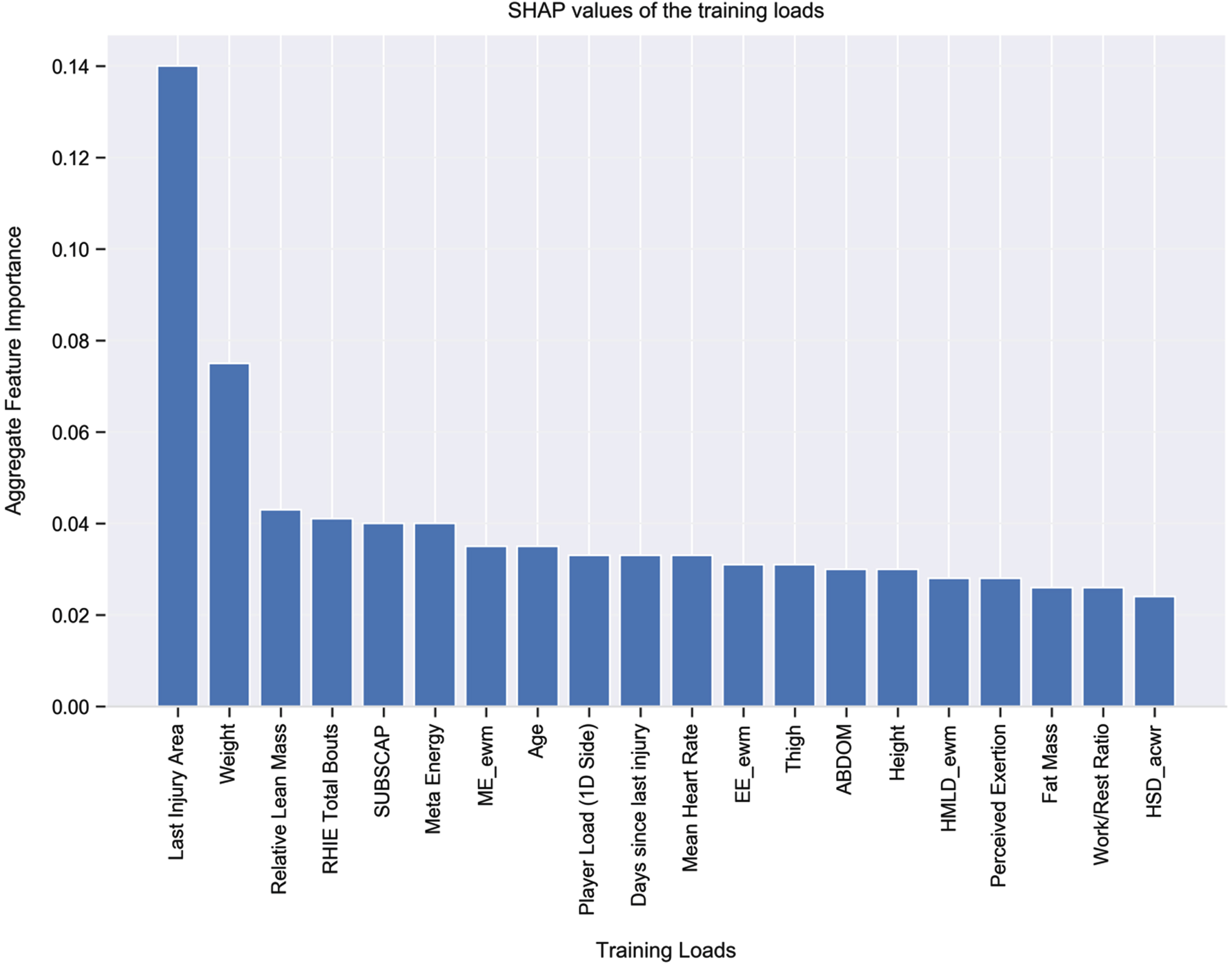
To interpret and visualize the output of each model and the contribution of each feature (i.e., training load) towards the model we used the Shaply Additive Explanations (SHAP) approach (Lundberg and Lee, 2017)—see Fig. 3. Higher SHAP values denote a higher contribution for that training load towards the model’s prediction. Given the relatively improved model, when using ANN over XGBoost, the following SHAP explanations relate to the model with ANN. With this in mind, the five most important features for injury risk in the train and validation data appear to be as follows: last injury area; exponential weighted moving average of meta energy; weight; meta energy; and age. We also used SHAP to examine the key features for injury risk at Months 1, 2, and 3 predicted by our trained ANN model (see Figs. 4–6). The two most important features that appeared in all models were last injury area and weight.
Fig. 3
Top 20 Features According to SHAP Values in The Training and Validation Data. Note: The variables in the model are listed from relatively the most important (left) to the least (right) important by their average global impact on the model. Each bar shows the mean absolute SHAP value for each variable, the higher the value, the higher the importance on the classification model (i.e., a higher probability of a positive prediction which is injury). The same applies for the Figs. 4, 5 and 6 as well.
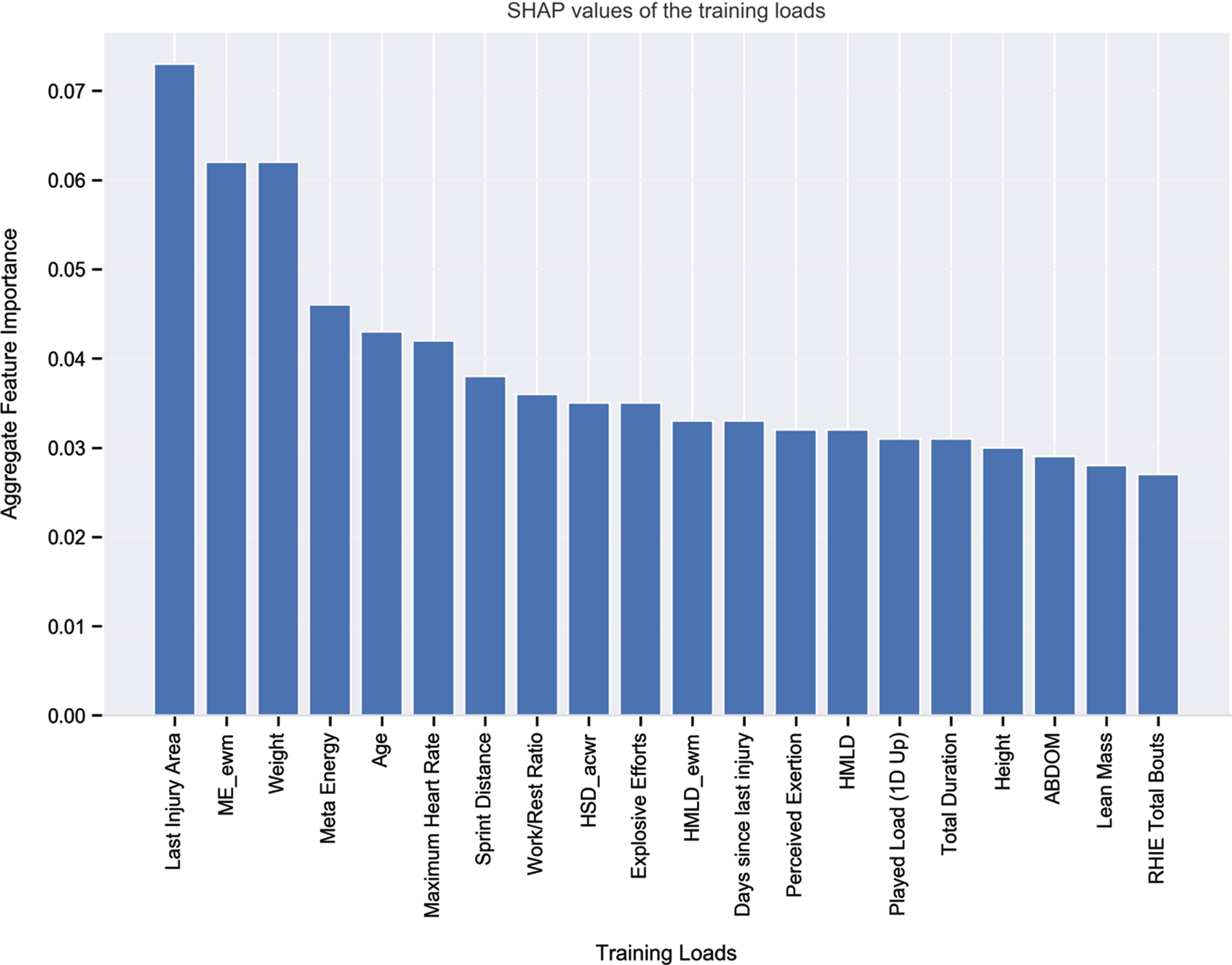
Fig. 4
Distribution of SHAP values for top features in The Training and Validation Data. Note: The variables in the model are listed from relatively the most important (top) to the least (bottom) important by their average global impact on the model. Each dot represents the SHAP value of an individual sample in the dataset which is plotted horizontally next to the feature name. We get an estimation of the distribution of the SHAP values per variable, saying that the higher the absolute value the higher the importance on the model prediction also, positive SHAP values represent a higher probability of a positive prediction (i.e., Injury).
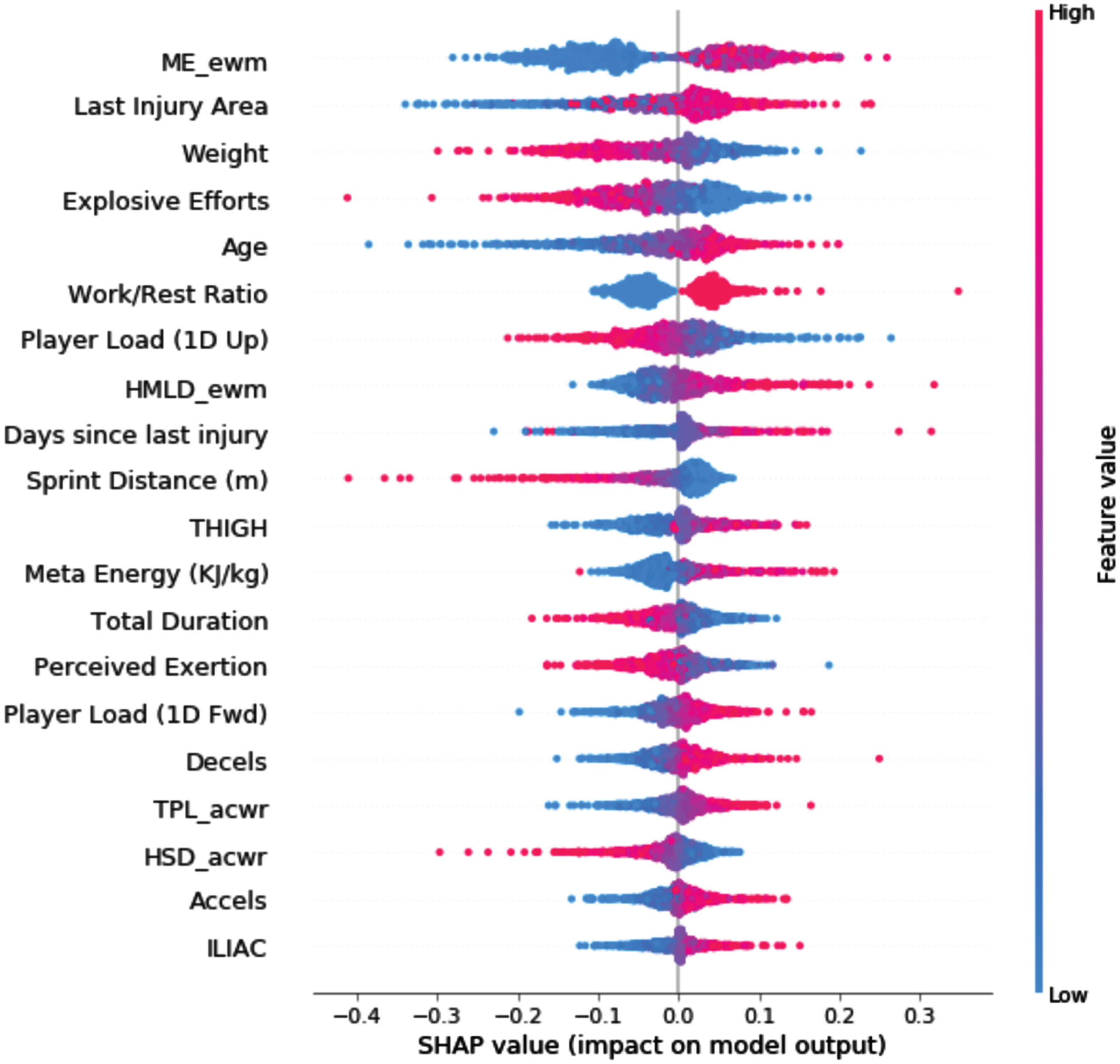
Fig. 5
Top 20 Features According to SHAP Values for Month 1.
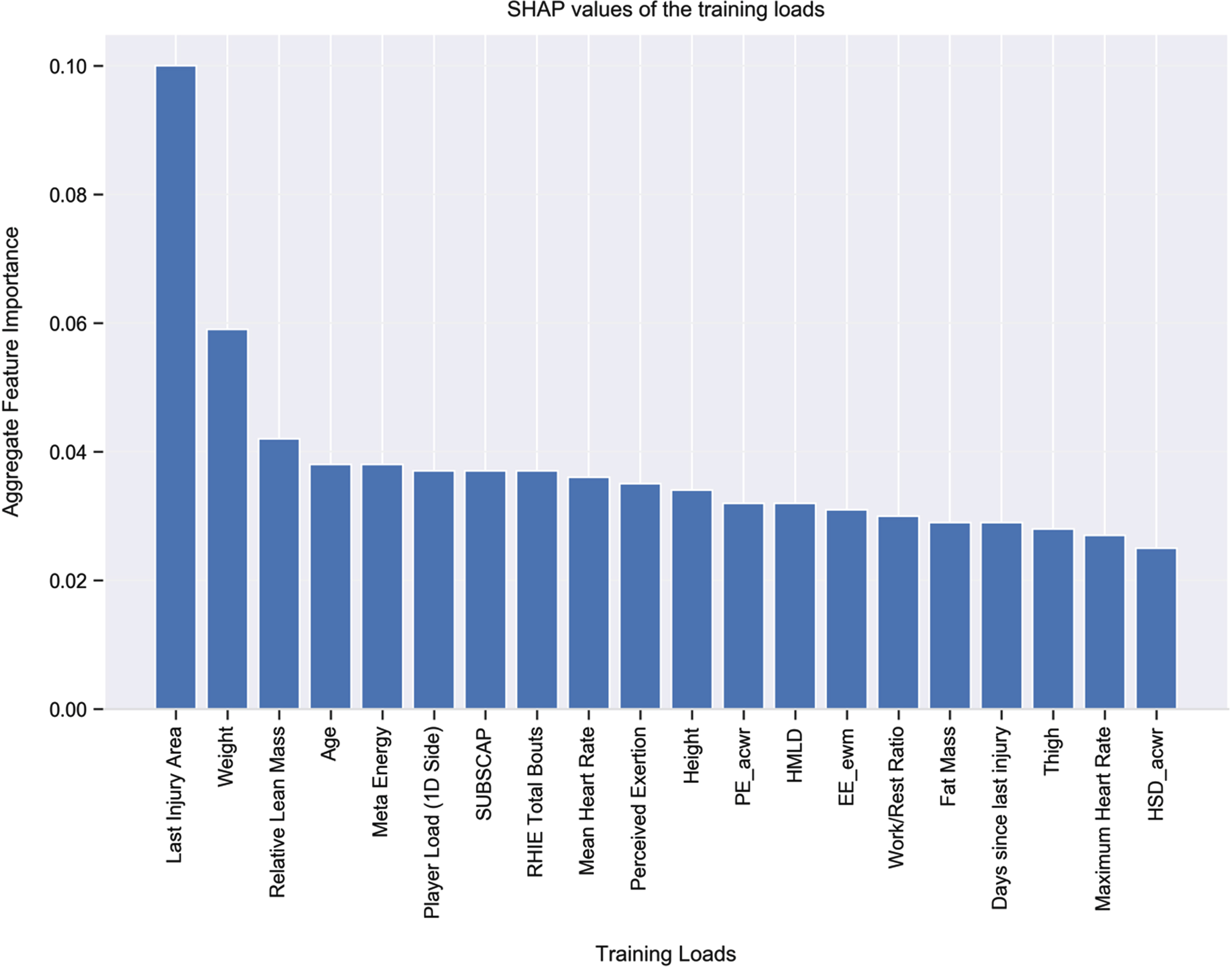
Fig. 6
Top 20 Features According to SHAP Values for Month 2.
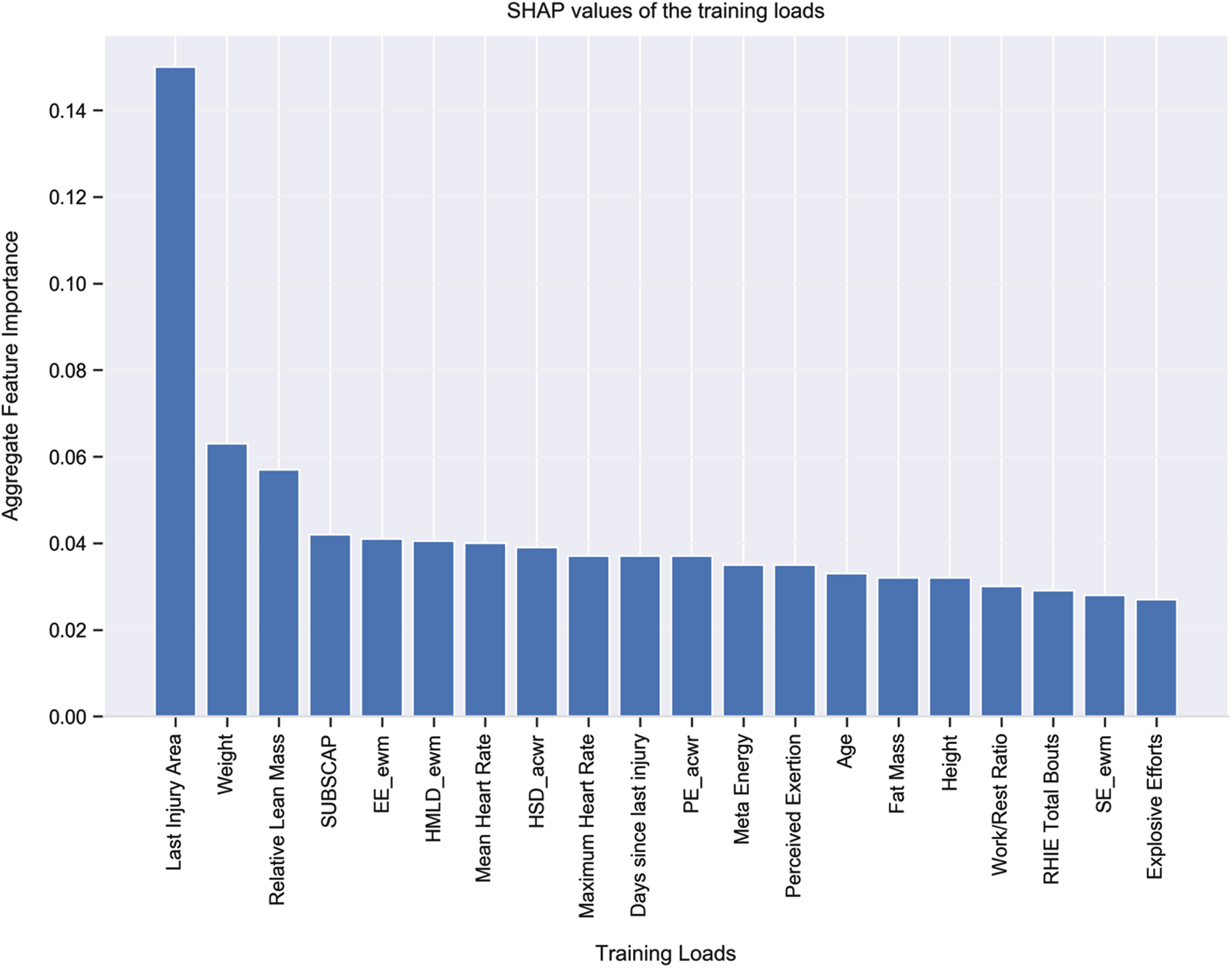
Fig. 7
The Top 20 Features According to SHAP Values for Month 3.
4Discussion
The purpose of this study was to use machine learning to examine the relationship between training load and soccer injury with a multi-season dataset from one English Premier League club. Our results demonstrated that two algorithms (XGBoost and ANN) provided the best results. Correctly predicting 26 of 37 injuries, XGBoost produced a precision value of 10% and recall of 73%; correctly predicting 28 of 37 injuries, ANN produced a precision value of 13% and recall of 77%. For the latter relatively better model using ANN, the most important features contributing to injury were “last injury area” and “weight”. Thus, although precision (i.e., the ratio of correctly predicted injuries to the total number of correctly and incorrectly predicted injuries) was relatively low (meaning that many of the model’s predicted injuries were not in fact injuries), values for recall (the ratio of correctly predicted injuries to the total observed injuries) were relatively high, suggesting precision suffered at the expense of being able to accurately predict most of the actual injury cases. If this model were used in an applied setting, the “false alarms” (those non-injuries that were predicted as injuries) might lead to some players being unnecessarily rested from training; at the same time, however, the model’s correctly predicted injuries would lead to most genuinely at-risk players rightfully being rested, and thereby saving players from injury and the club from losing players to injury, with the concomitant selection problems, rehabilitation time, and financial impact. Finally, the ANN model produced low false negatives, suggesting that if the model predicts that a player will not be injured, this is likely to be the case.
Injury prediction perspectives. Our study used a very high dimensional and highly imbalanced, overlapped dataset. Although ANN has been successfully employed to deal with such high dimensional, overlapped datasets in other fields of artificial intelligence (such as in object detection, image recognition, speech recognition, text processing, recommendation systems, and time series model building: Bohr and Memarzadeh, 2020; Emmert-Streib et al., 2020; Johnson and Khoshgoftaar, 2019), it has never been used for soccer injury prediction. In the present study, ANN out-performed “state-of-the-art” XGBoost, with better recall and precision values. In attempting to counter class imbalance in the present study’s dataset, data oversampling (i.e., Smote), in combination with setting the weights for injury at nine (for XGBoost) and eleven (for ANN) times higher than for non-injury (termed a cost-sensitive classification), we were able to maximize the accurate prediction of injuries.
Injury prediction is based on analysis of longitudinal data, with the goal of being able to accurately predict injuries in some pre-defined upcoming period of days. Thus, in order to ensure the independence of test and train data, in addition to the usual cross-validation, we also evaluated our models on unseen future (test) data. In terms of data pre-processing, differently from Lopez-Valenciano et al. (2018) and Ayala et al. (2019) who imputed missing values using the mean, we used different imputation techniques for different types of training loads. For example, some physical training load variables (such as weight and body fat percentage) are not measured on a daily basis, even though they naturally increase or decrease gradually over time. Imputing the missing values of these features by using the mean or the most frequent values may not reflect well the actual values over time. To combat this potential inaccuracy, we used interpolation for imputing the missing values of those time-dependent features. In a similar way, to better replicate the most practical and reasonable values with our GPS measures, ACWR, MSWR, and EWMA, we imputed missing values using k-nearest neighbor or weekly mean values.
Explainability. Compared with white-box machine learning models, “black-box” models, like those examined in the present research (i.e., XGBoost and ANN), can provide better predictive performance, but at the expense of being difficult to interpret and understand. With black-box models, then, additional post hoc methods are needed to interpret and understand results (Loyola-Gonzalez, 2019). Thus, in terms of the explainability of our model, we present (based on SHAP explanations) the important features (i.e., training loads) in Figs. 3–6. Last injury area was a key feature in the ANN model—37% of injured players had a previous record of thigh injury, 30% had a previous record of knee injury, 16% had a previous record of lower leg injury, and 17% did not have any previous record of injury. Further, 84% of injuries occurred in those with body weights between 73 kg and 85 kg. It is worthy of note that, despite the power of SHAP explanations, the output from such global explanations can sometimes be misleading. For example, in our main dataset 122 of 133 injuries, and in our dataset D 334 out of 378 injuries, occurred when the exponential weighted moving average (EWMA) of Meta Energy exceeded a value of 6.14. On the contrary, with our test data (i.e., those data not included in the training and validation dataset), of 530 data points, there were no data points for which EWMA of Meta Energy exceeded a value of 6.14. Thus, although (see Fig. 3) EWMA of Meta Energy was one of the top three features in the training and validation data, it failed to emerge as an important feature in Months 1–3 (as can be seen in Figs. 4–6). What this means is that, despite its apparent importance during training and validation, EWMA of Meta Energy plays no major role in terms of explainability of the test data. Building from the above, if we had divided our entire dataset on a 10% train-test split basis (rather than using our process of testing on later data), we would have likely concluded that EWMA of Meta Energy plays a more prominent role in terms of explainability than it actually does in real life. Finally, it is also worth noting that in our data, values for the ACWR (the most well-researched model of injury monitoring in soccer) appeared to differ from those noted in the existing literature. Thus, in contrast with research demonstrating, for example, that values in excess of 2 (Bowen et al., 2019) or less than 1 (Rossi et al., 2018) might lead to greater injury risk, the majority of injuries in our data occurred when ACWR values were between 0.5 and 1.5.
Practical applications. The models developed in this study could be used by clubs and practitioners to calculate the probability of a player getting injured in the next seven days. With the use of explainability (via SHAP), practitioners would also be well-positioned to have an essence of the cause of injuries predicted by the models. The results from the present study cannot be directly compared with other studies into soccer injury, because, unlike those studies, we used a multi-season dataset with a very high imbalance ratio. However, in seeking to make comparisons, we reproduced as closely as possible, with our data, the analysis strategy from two other well-regarded soccer injury studies—the work of Rossi et al. (2018) and Vallance et al. (2020). In attempting to predict injuries in the next day and in the next seven-day window, we used all the possible similar features (i.e., the training load variables) from Rossi et al. (2018) and Vallance et al. (2020) that were also available in our data, and followed their methods with regard to data pre-processing, feature selection, feature extraction, balancing techniques, model training, hyperparameter optimization, along with the model evaluation and validation techniques, where specified. In reproducing the work of Rossi et al. (2018), we used the Recursive Feature Elimination (Guyon et al., 2002) as the feature selection technique which yielded just one feature in our data, and the prediction based on that one feature was not as high as the results reported by Rossi at el. (2018). In reproducing the work of Vallance et al. (2020), we used the Bayesian optimization hyperparameter technique with our data, which predicted most of the non-injuries. Rossi et al. (2018) reported as their best algorithm Decision Tree, and Vallance et al. (2020) reported as their best algorithms k-nearest neighbors, random forest, decision tree, and XGBoost—conversely, only XGBoost performed well with our data. It is important to note that the differences we noted in our data are completely normal, and should be expected. All clubs have different philosophies and unique ways of handling their training load data. As a result, the number of training loads used and the training programs employed at clubs are frequently quite different. And thus, the choice of the best performing machine learning algorithm for each dataset is likely dependent on the context and the quality of those data.
Strengths and limitations. The present research had some notable strengths. First, to the best of our knowledge this is the first study that has considered multi-season data with elite male soccer players from the English Premier League. Second, we included many types of training loads, including GPS measures, physical and psychological loads, personal information, as well as ACWR, MSWR, and EWMA of certain training load variables (See Table 1). Third, we also created features—such as last injury area and days since the last injury—which appeared to enhance the predictive utility of our machine learning model and were among the most important injury predictors. Fourth, the proposed seven-day injury prediction window is unique to our study—and aligned well with the notion that English Premier League are generally played every seven days. Fifth, our use of ANN was a novel addition, which appeared marginally more effective than the state-of-the-art XGBoost in predicting injuries. All the above led us to conclude that the most important features in our study were “last injury area” and “weight”, which are very general—these two features are monitored in almost every sporting organization to evaluate injury risk among players, and thus in practical terms the present research has genuinely real-world application. Against the backdrop of these many strengths, a major limitation for the process used in the present research (as is true for many machine learning processes) is that when new data are available, the model would have to be retrained, and thus the predictions may then vary. That said, given that we were able to demonstrate that machine learning models trained on a highly multi-dimensional and imbalanced dataset can indeed predict and explain injuries to address the needs of a professional soccer club, different clubs and organizations could use our approach with amendments to the feature set as required.
Future Research. As noted above, a limitation of the present research is the need to retrain the models when new data become available. Thus, a future research avenue could be to develop automation of the model training process with continuously incoming injury data, so that the models adapt to this new information. This would seem particularly important in soccer, wherein changes in training processes, team members, and injuries mean that the underlying distribution of the data does not remain constant across seasons. We believe that this limitation could be addressed by using adaptive streaming predictive methods (Yang, Manias and Shami, 2021), and we encourage future research to examine this further.
4Conclusions
Using a highly imbalanced and high dimensional, overlapped, multi-season dataset from an English Premier League soccer club, we were able to predict soccer injuries with high recall. Our novel use of ANN in combination with explainable artificial intelligence also demonstrated its potential to unearth effective insights into the workload-injury relationship. Our data pre-processing techniques such as unique missing value imputation techniques, new features creation, handling of the high imbalance in non-injuries and injuries, train-validation process alongside testing of models on real-life in-coming data, and improving recall and precision techniques all have potential to lay the foundation for future research to employ machine learning in a more practical way to predict injuries.
Appendix
Acknowledgment
Contributions
Aritra Majumdar, Rashid Bakirov, Dan Hodges, and Tim Rees developed the initial idea for the article. Aritra Majumdar performed the literature search and all analyses. Aritra Majumdar wrote the first draft of the article. Aritra Majumdar, Rashid Bakirov, and Tim Rees critically revised the work. Dan Hodges and Sean McCullagh commented on the final draft of the work. All authors read and approved the final version of the manuscript prior to submission.
This work was supported by funding awarded to the first author by AFC Bournemouth and Bournemouth University.
Corresponding author
Correspondence to Aritra Majumdar.
Competing interests
Aritra Majumdar received funding from AFC Bournemouth and Bournemouth University. Dan Hodges is a former employee of AFC Bournemouth and currently working at Newcastle United FC. Sean McCullagh is a first team sport scientist at AFC Bournemouth. Rashid Bakirov and Tim Rees are supervisors of Aritra Majumdar, who has received funding from AFC Bournemouth and Bournemouth University. Aritra Majumdar, Rashid Bakirov, Dan Hodges, Sean McCullagh, and Tim Rees declare that they have no competing interests.
References
1 | Ayala F. , López-Valenciano A. , Gámez Martín J.A. , De Ste Croix M. , Vera-Garcia F. , García-Vaquero M. , Ruiz-Pérez I. , Myer G. , (2019) , A preventive model for hamstring injuries in professional soccer: Learning algorithms. [online], International Journal of Sports Medicine, 40: (05), 344–353. doi: 10.1055/a-0826-1955 |
2 | Belle V. , Papantonis I. , 2020, Principles and practice of explainable machine learning. arXiv:2009.11698 [cs, stat]. [online]Available at: https://arxiv.org/abs/2009.11698 [Accessed 22 Jul. 2022]. |
3 | Bourdon P.C. , Cardinale M. , Murray A. , Gastin P. , Kellmann M. , Varley M.C. , Gabbett T.J. , Coutts A.J. , Burgess D.J. , Gregson W. , Cable N.T. , (2017) , Monitoring athlete training loads: Consensus statement, International Journal of Sports Physiology and Performance, 12: (s2), S2-161–S2-170. doi: 10.1123/ijs2017-0208 |
4 | Bowen L. , Gross A.S. , Gimpel M. , Bruce-Low S. , Li F.-X. , 2019, Spikes in acute:chronic workload ratio (ACWR) associated with a 5–7 times greater injury rate in English Premier League soccer players: a comprehensive 3-year study. British Journal of Sports Medicine, [online] p.bjsports-2018-099422. doi: 10.1136/bjsports-2018-099422 |
5 | Chawla N.V. , Bowyer K.W. , Hall L.O. , Kegelmeyer W.P. , (2002) , SMOTE: Synthetic minority over-sampling technique, Journal of Artificial Intelligence Research, 16: (16), 321–357. doi: 10.1613/jair.953 |
6 | Chen T. , Guestrin C. , 2016, XGBoost: A scalable tree boosting system. Proceedings of the 22nd ACM SIGKDD International Conference on Knowledge Discovery and Data Mining –KDD ’16. [online] doi: 10.1145/2939672.2939785 |
7 | Chen T. , Guestrin C. , 2016, XGBoost: A scalable tree boosting system. Proceedings of the 22nd ACM SIGKDD International Conference on Knowledge Discovery and Data Mining –KDD ’16. [online] doi: 10.1145/2939672.2939785 |
8 | Eliakim E. , Morgulev E. , Lidor R. , Meckel Y. , (2020) , Estimation of injury costs: financial damage of English Premier League teams’ underachievement due to injuries., BMJ Open Sport & Exercise Medicine, [online] 6: (1), e000675. doi: 10.1136/bmjsem-2019-000675 |
9 | Gupta S. , Gupta A. , (2018) , Handling class overlapping to detect noisy instances in classification, The Knowledge Engineering Review, 33: . doi: 10.1017/s0269888918000115 |
10 | Halson S.L. , (2014) , Monitoring training load to understand fatigue in athletes, Sports Medicine, 44: (S2), 139–147. doi: 10.1007/s40279-014-0253-z |
11 | Hulin B.T. , Gabbett T.J. , Blanch P. , Chapman P. , Bailey D. , Orchard J.W. , (2013) , Spikes in acute workload are associated with increased injury risk in elite cricket fast bowlers, British Journal of Sports Medicine, [online] 48: (8), 708–712. doi: 10.1136/bjsports-2013-092524 |
12 | Ibrahimović M. , Mustafović E. , Causevic D. , Alić H. , Jelešković E. , Talović M. , (2021) , Injury rate in professional football: A systematic review, International Journal of Physical Education, Fitness and Sports, 10: (2), 52–63. doi: 10.34256/ijpefs2126 |
13 | Impellizzeri F.M. , Woodcock S. , Coutts A.J. , Fanchini M. , McCall A. , Vigotsky A.D. , (2021) , What Role Do Chronic Workloads Play in the Acute to Chronic Workload Ratio? Time to Dismiss ACWR and Its Underlying Theory, Sports Medicine, 51: (3), 581–592. doi: 10.1007/s40279-020-01378-6 |
14 | Jones A. , Jones G. , Greig N. , Bower P. , Brown J. , Hind K. , Francis P. , (2019) , Epidemiology of injury in English professional football players: A cohort study, Physical Therapy in Sport, 35: , 18–22. doi: 10.1016/j.pts2018.10.011 |
15 | Kalkhoven J.T. , Watsford M.L. , Coutts A.J. , Edwards W.B. , Impellizzeri F.M. , (2021) , Training Load and Injury: Causal Pathways and Future Directions, Sports Medicine, 51: (6), 1137–1150. doi: 10.1007/s40279-020-01413-6 |
16 | Kampakis S. , 2016, Predictive modeling of football injuries. [online] Available at: https://arxiv.org/pdf/1609.07480.pdf. |
17 | Kiesow H. , Spreng R.N. , Holmes A.J. , Chakravarty M.M. , Marquand A.F. , Yeo B.T.T. , Bzdok D. , (2021) , Deep learning identifies partially overlapping subnetworks in the human social brain, Communications Biology, [online] 4: (1), 1–14. doi: 10.1038/s42003-020-01559-z |
18 | López-valenciano A. , Ayala F. , Puerta Jos M. , De Ste Croix M.B.A. , Vera-Garcia F.J. , Hernández-Sánchez S. , Ruiz-Pérez I. , Myer G.D. , (2018) , A preventive model for muscle injuries, Medicine & Science in Sports & Exercise, 50: (5), 915–927. doi: 10.1249/mss.0000000000001535 |
19 | Loyola-Gonzalez O. , (2019) , Black-Box vs. White-Box: Understanding their advantages and weaknesses from a practical point of view, IEEE Access, 7: , 154096–154113. doi: 10.1109/access.2019.2949286 |
20 | Lundberg S. , Lee S.-I. , 2017, A Unified approach to interpreting model predictions. arXiv:1705.07874 [cs, stat]. [online] Available at: https://arxiv.org/abs/1705.07874. |
21 | Majumdar A. , Bakirov R. , Hodges D. , Scott S. , Rees, T. , (2022) , Machine learning for understanding and predicting injuries in football, Sports Medicine –Open, 8: (1), 73. doi: 10.1186/s40798-022-00465-4 |
22 | Mehlig B. , 2019, Artificial neural networks. arXiv:1901.05639 [cond-mat, stat]. [online] Available at: https://arxiv.org/abs/1901.05639. |
23 | Mehlig B. , 2019, Artificial neural networks. arXiv:1901.05639 [cond-mat, stat]. [online] Available at: https://arxiv.org/abs/1901.05639. |
24 | Naglah A. , Khalifa F. , Mahmoud A. , Ghazal M. , Jones P. , Murray T. , Elmaghraby A.S. , El-baz A. , 2018, Athlete-customized injury prediction using training load statistical records and machine learning. [online] IEEE Xplore. doi: 10.1109/ISSPIT.2018.8642739 |
25 | Oliver J.L. , Ayala F. , De Ste Croix M.B.A. , Lloyd R.S. , Myer G.D. , Read P.J. , (2020) , Using machine learning to improve our understanding of injury risk and prediction in elite male youth football players, Journal of Science and Medicine in Sport, 23: (11), 1044–1048. doi: 10.1016/j.jsams.2020.04.021 |
26 | Owoeye O.B.A. , VanderWey M.J. , Pike I. , (2020) , Reducing injuries in soccer (football): An umbrella review of best evidence across the epidemiological framework for prevention, Sports Medicine –Open, 6: (1), 46. doi: 10.1186/s40798-020-00274-7 |
27 | Rahnama N. , (2011) , Prevention of football injuries, International Journal of Preventive Medicine, [online] 2: (1), 38–40. Available at: https://www.ncbi.nlm.nih.gov/pmc/articles/PMC3063461/. |
28 | Rommers N. , Rössler R. , Verhagen E. , Vandecasteele F. , Verstockt S. , Vaeyens R. , Lenoir M. , D’hondt E. , Witvrouw E. , (2020) , A machine learning approach to assess injury risk in elite youth football players, Medicine & Science in Sports & Exercise, 52: (8), 1745–1751. doi: 10.1249/mss.0000000000002305 |
29 | Rossi A. , Pappalardo L. , Cintia P. , (2021) , A narrative review for a machine learning application in sports: An example based on injury forecasting in soccer, Sports, [online] 10: (1), 5. doi: 10.3390/sports10010005 |
30 | Rossi A. , Pappalardo L. , Cintia P. , Iaia F.M. , Fernàndez J. , Medina D. , (2018) , Effective injury forecasting in soccer with GPS training data and machine learning, PLOS ONE, 13: (7), e0201264. doi: 10.1371/journal.pone.0201264 |
31 | Sáez J.A. , Galar M. , Krawczyk B. , (2019) , Addressing the overlapping data problem in classification using the one-vs-one decomposition strategy, IEEE Access, [online] 7: , 83396–83411. doi: 10.1109/ACCESS.2019.2925300 |
32 | Shahee S.A. , Ananthakumar U. , (2021) , An overlap sensitive neural network for class imbalanced data, Data Mining and Knowledge Discovery, 35: (4), 1654–1687. doi: 10.1007/s10618-021-00766-4 |
33 | Tang W. , Mao K.Z. , Mak L.O. , Ng G.W. , 2010, Classification for overlapping classes using optimized overlapping region detection and soft decision. [online] IEEE Xplore. doi: 10.1109/ICIF.2010.5712008 |
34 | Vallance E. , Sutton-Charani N. , Imoussaten A. , Montmain J. , Perrey S. , (2020) , Combining internal- and external-training-loads to predict non-contact injuries in soccer, Applied Sciences, 10: (15), 5261. doi: 10.3390/app10155261 |
35 | Van Eetvelde H. , Mendonça L.D. , Ley C. , Seil R. , Tischer T. , (2021) , Machine learning methods in sport injury prediction and prevention: A systematic review, Journal of Experimental Orthopaedics, 8: (1). doi: 10.1186/s40634-021-00346-x |
36 | Venturelli M. , Schena F. , Zanolla L. , Bishop D. , (2011) , Injury risk factors in young soccer players detected by a multivariate survival model, Journal of Science and Medicine in Sport, 14: (4), 293–298. doi: 10.1016/j.jsams.2011.02.013 |
37 | Bohr A. , Memarzadeh K. , (2020) , The rise of artificial intelligence in healthcare applications, Artificial Intelligence in Healthcare 25–60. doi: 10.1016/B978-0-12-818438-7.00002-2 |
38 | Emmert-Streib F. , Yang Z. , Feng H. , Tripathi S. , Dehmer M. , (2020) , An introductory review of deep learning for prediction models with big data, Frontiers in Artificial Intelligence, 3: . doi: 10.3389/frai.2020.00004 |
39 | Johnson J.M. , Khoshgoftaar T.M. , (2019) , Survey on deep learning with class imbalance, Journal of Big Data, 6: (1). doi: 10.1186/s40537-019-0192-5 |
40 | Guyon I. , Weston J. , Barnhill S. , Vapnik V. , (2002) , Gene selection for cancer classification using support vector machines, Machine Learning, 46: , 389–422. doi: 10.1023/A:1012487302797 |
41 | Yang L. , Manias D.M. , Shami A. , 2021, PWPAE: An ensemble framework for concept drift adaptation in IoT data streams. 2021 IEEE Global Communications Conference (GLOBECOM). doi: 10.1109/globecom46510.2021.9685338 |


