
Evaluating NBA end-of-game decision-making
Abstract
This paper introduces a probabilistic method to evaluate the tactical decisions players and coaches make at the end of NBA games. For the purposes of this research, these decisions include whether to shoot a two-point or three-point field goal for the offensive team and whether to intentionally foul for the defensive team. With a win probability model built using logistic regression and player statistics, the optimal decision for both teams in a given possession is found. The End-of-game Tactics Metric (ETM) is the difference between the win probability of the optimal decision and the win probability of the actual decision. This research extends beyond current applications of win probability models to evaluate the actual on-court decision as opposed to evaluating the result of a possession.
To evaluate the usefulness of ETM, the winning percentage of teams in games decided by a margin of five points or fewer can be compared with the mean ETM difference between a team and its opponent. The correlation coefficient of the relationship is -0.64. When combined with other variables that affect winning percentage in close games, a linear regression on those explanatory variables has an adjusted R2 value of 0.79. This analysis shows that the ETM difference has a significant effect on winning close games, despite having little reliance on player performance.
1Introduction
Since the beginning of basketball, coaches and players have been making decisions during play to increase the chances of their team winning. While the majority of these decisions concern playing style, offensive sets, and defensive schemes, the end of the game presents opportunities for teams to executecertain tactics.
When trailing late in the game, teams intentionally foul in order to get the ball back quickly, incurring the cost of two free throw attempts from the opponent. Teams also employ the intentional foul tactic while leading by three points in the final seconds of a game, instead of allowing a possible three-point field goal. Offensive tactics consist of the timing and type of field goal to attempt.
This paper presents the development of an end-of-game tactics metric (ETM) to inform in-game decision-making. ETM relies on an NBA win probability model finding the difference between the win probability of the optimal and actual tactic for a given possession. As such, ETM represents the amount of win probability a team gives up by employing adifferent tactic than the optimal one.
Impressive research has been conducted that supports moving away from the results-based view of basketball to a more probabilistic view. Beuoy (2015) developed an in-game NBA win probability model, serving as the driver for several metrics and ad-hoc studies. This win probability model motivates the win probability model in this paper. Goldsberry et al. (2014) introduced the idea of expected possession value (EPV) that measures the expected number of points for a possession given time, player with the ball, and defensive makeup and spatial orientation. While EPV has similarities to the ETM introduced in this paper, EPV requires much more granular data and, therefore, may be difficult to use in the context of informing in-game decision making. ETM uses team statistics to find an optimal tactic for a possession, but the general algorithm can be altered with an EPV-like metric for specific offensive sets, for example. Burke (2010) applied win probability and expected points in football and Tango (2007) pioneered this concept in baseball.
In this paper, win probability and the probability of success for different offensive and defensive tactics combine to form several branches of post-possession win probability from which to choose. By modeling the state of the game as a function of possession, time remaining, and score differential, the game can be viewed as a Markov chain with transition probabilities based on team statistics. The following sections detail the mathematics behind ETM, the resulting ETM statistics for the 2015-2016 NBA season, and ETM applications.
2Methodology
This section details the development of a win probability model for the last three minutes of an NBA game. With this, each possession of a basketball game has an associated win probability. This idea then leads directly to the definition of ETM.
2.1Win probability model
The win probability model in this paper, restricted to the last three minutes of the game, uses time remaining, score differential, possession, and point spread. The data consist of NBA regular season play-by-play descriptions from 2011 to 2015 gathered from stats.nba.com (Luo, 2017). The point spread data come from sportsdatabase.com. The win probability model is built using the statistical modeling technique of logistic regression. Given any game situation, the model takes the state of the game and generates a win probability describing the chances of winning for both teams.
Eq. 1 shows the general logistic regression function of the win probability model,
(1)
where P (W) is the win probability for the team with possession, βi is the coefficient of the ith term, S is the score differential relative to the team with possession,
The features in the model consist of nonlinear functions of score differential and time remaining in the game. The motivation behind using these nonlinear functions is the intuition that these variables combine nonlinearly to affect the probability of winning. Many features of this nature were tried with the validation set guiding the choice of the final model via maximum likelihood.
The model was then run on an independent test set. On these test data with a win probability cutoff of 0.5 for class assignment, the model has a precision of 92.3% and a recall of 90.9%, with an overall accuracy of 92.5%. These values indicate that the logistic regression model provides a reasonable estimate of in-game win probability.
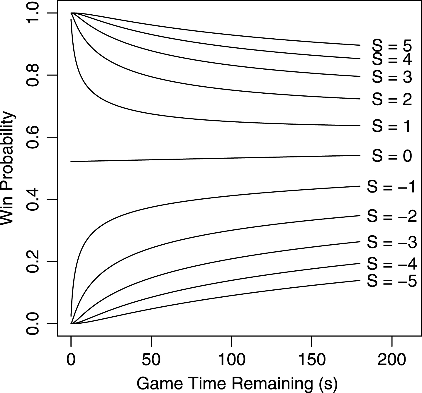
Figure 1 provides an illustration of how the logistic regression model maps to in-game win probability given different game states. The figure contains the win probability plots of a team with a given score differential and how the win probability changes within the last three minutes. For each time point, the win probability corresponds to a team starting possession at that moment with the circumstances shown in the figure. This plot reveals several features of the win probability model. As the score differential gets more positive, the resulting increase in win probability gets smaller, which agrees with intuition as the win probability asymptotically approaches one. Smaller score differentials have extreme win probability behavior as the time remaining approaches zero.
Fig.1
Win probabilities for different score differentials S and game time remaining for a team with possession and a point spread of zero.
2.2End-of-game tactics metric
The win probability model serves as the foundation for ETM because, at the beginning of each possession, both teams have an initial win probability and a set of choices to make. At a tactical level, these choices include whether to shoot a two-point or three-point field goal for the offensive team and whether to intentionally foul for the defensive team, which are the only decisions evaluated in this study. The timing of these decisions also factor into the decision-making process. The possibility of a turnover or free throws on a shooting foul exists, but these are not explicit choices made by teams. The power of ETM lies in the ability to calculate the optimal decision and judge a team’s actual decision relative to the optimal one.
The Chapman-Kolmogorov equations allow for the calculation of the win probability of a team after a given decision is made. In this context, the equation states that the probability of winning a game after making a decision k is the sum of the probability of all of the possible outcomes of that decision multiplied by the probability of winning after those outcomes. In equation form, this becomes,
(2)
where P (W) k is the probability of winning after making decision k, Pj is the probability of score differential j occurring after making decision k, P (W) j is the probability of winning if score differential j occurs after making decision k, and J is the number of possible score differentials of the decision k. The decisions include k ∈ (2 - pointshot, 3 - pointshot) for the offensive team and the decisions include k ∈ (Intentionallyfoul, Nofoul) for the defensive team. The win probability term of Eq. 2 comes directly from the win probability model. The Pj term comes from evaluating how all of the different outcomes of a decision can result in score differential j. For example, for the score differential to remain the same after a decision to shoot a two-point field goal, this can occur if the team misses the field goal attempt, turns the ball over, or misses both free throw attempts followinga shooting foul (for simplicity, this model ignores getting fouled during a three-point field goal attempt). The probabilities of all of these outcomes come from team statistics, including two-point field goal percentage, three-point field goal percentage, turnover percentage, free throw percentage, rebound percentage, and foul percentage. These statistics vary by team and this study uses team statistics rather than aggregated league averages. Eq. 2 evaluates the transition of the current state of the game to all other possible future states of the game, after one possession.
With the ability to evaluate the decision-making of teams both offensively and defensively, ETM can now be defined as,
(3)
3Results
For aggregate ETM results, the above models used play-by-play data from the 2015-2016 NBA season from basketball-reference.com. Team fouls per possession come from teamrankings.com. The models only used data from games that ended with a score differential within five points so as to focus on games where the outcome was certainly in question in the last three minutes. In addition, a shooting weight for field goal percentage is applied to team shooting percentages to account for the effect of the shot clock on shooting percentage. This was found by fitting a quadratic function to team shooting percentage by shot clock time from nba.com/stats for the 2014-2015 NBA season. This shooting weight is set to one with fewer than 24 seconds remaining when the shot clock is off.
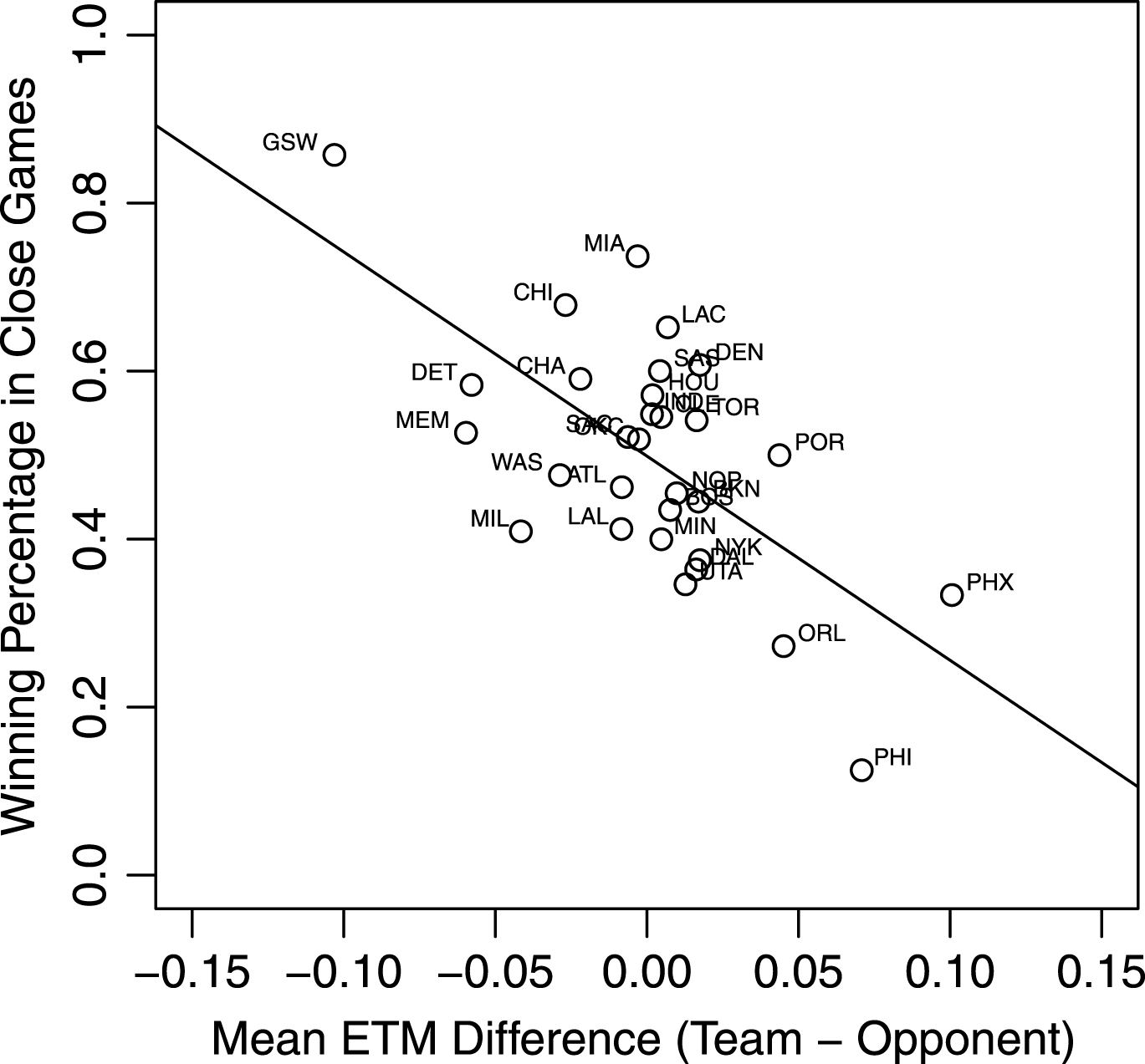
The results include games ending with a score differential of five points or fewer and periods that lead to an additional overtime period. The results consider the final 180 seconds of such periods. Fig. 2 shows the winning percentage in close games versus the average difference between the ETM of a team and its opponent. The line in Fig. 2 is a least-squares fit of the relationship between the two plotted variables. The correlation coefficient of this relationship is -0.64, meaning that higher win probability in close games is associated with a more negative ETM difference. The variability exhibited in Fig. 2 stems from winning percentage being related to more than just decision-making in the final minutes of close games. Winning percentage in such games also depends on execution in many facets of the game on the offensive and defensive sides of the ball. When combined with other variables that affect winning percentage in close games, a linear regression on those explanatory variables has an adjusted R2 value of 0.79. These other explanatory variables include the win probability of a team at the start of the remaining three minutes, the difference in field goals made between teams, and the difference in fouls committed between teams.
Fig.2
Winning percentage in close games versus mean ETM difference for NBA teams during the 2015-2016 season overlaid with the least-squares regression line.
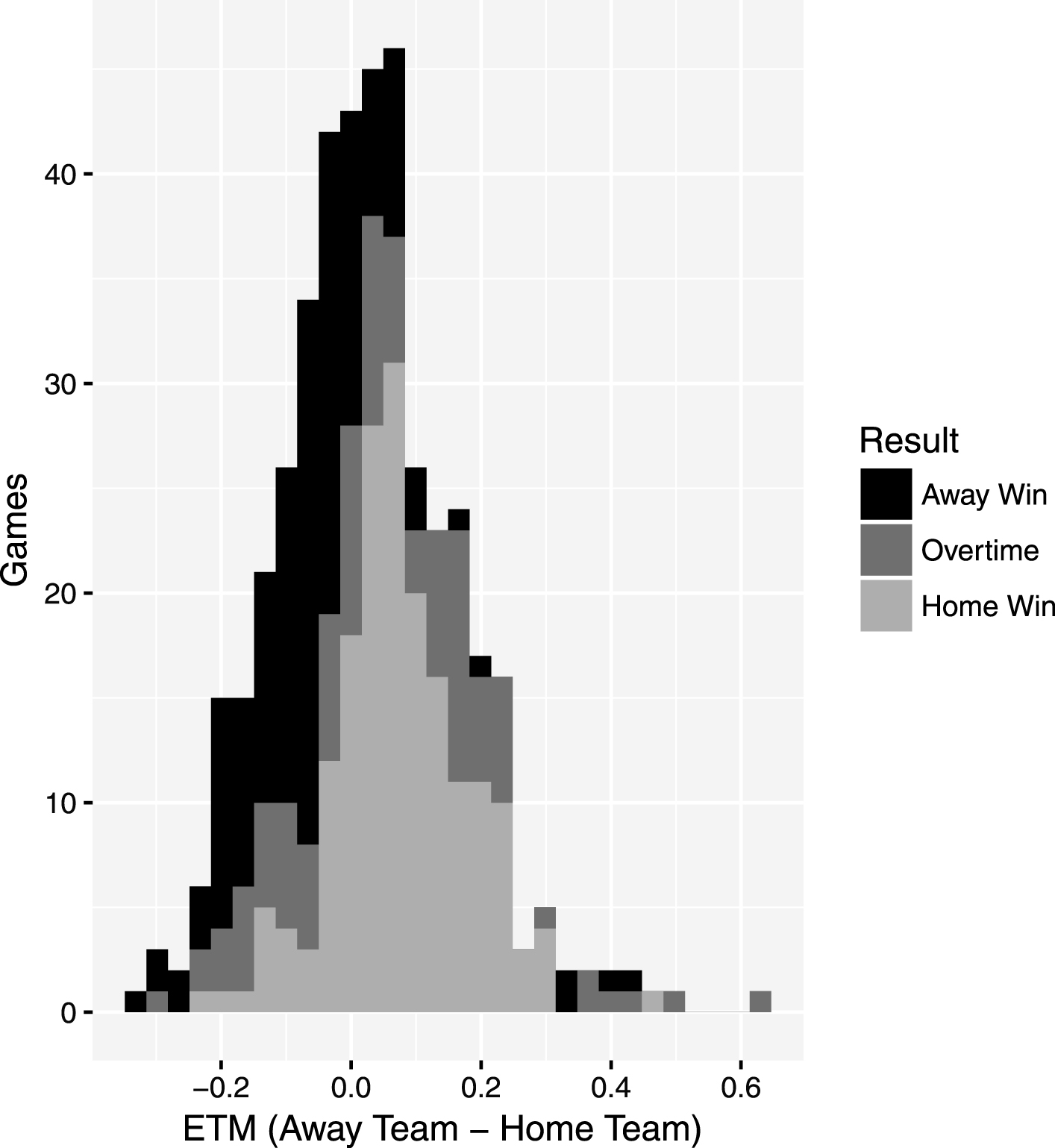
While Fig. 2 shows a relationship between ETM and winning percentage at an aggregate level, Fig. 3 shows a more granular game-by-game relationship of ETM and winning percentage. The histogram shows an albeit noisy trend of the team with a lower ETM enjoying a higher winning percentage. The source of the noise is almost certainly multidimensional, with possible sources being few games of a certain ETM difference and performance variables, as discussed above. Considering the results presented, ETM difference has a significant effect on winning close games, despite having no reliance on the outcome of aparticular play.
Fig.3
Histogram showing the results of close games in the 2015-2016 NBA season. The general trend shows that the team with a lower ETM can expect a higher winning percentage.
4ETM applications
4.1“Fouling Up-3”
The “Fouling Up-3” tactic is used by teams leading by three points in the final seconds of a game in order to force two free throw attempts instead of a three-point field goal attempt. The tactic has been heavily debated, but analyses and studies on the topic tend to be heuristic in nature (Annis, 2006). While these studies provide value, statistical modeling efforts like ETM can provide more insight.
Using ETM and win probability to examine this tactic is quite straightforward. Consider a team on defense leading by three points. This team has the option to intentionally foul or play conventional defense. Fig. 4 shows the win probability for each option of a defensive team winning by three points and the possession beginning at a given time.
Fig.4
Win probability for a team winning by three points without possession for two tactics. The win probability of the intentional foul tactic exceeds the win probability of playing conventional defense beginning at nine seconds remaining.
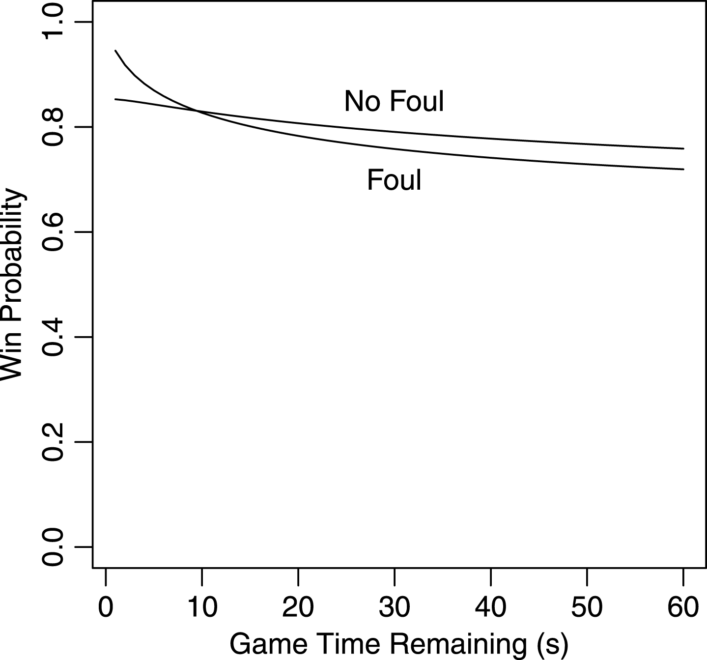
Notice how the defensive win probability changes throughout the last 36 seconds of the game in Fig. 4. With 36 seconds remaining, the conventional defensive tactic win probability is 3.5 percentage points higher than the intentionally fouling tactic. However, the intentionally fouling tactic becomes the more optimal tactic around nine seconds remaining. With one second remaining, intentionally fouling is 9.2 percentage points higher than theconventional defensive tactic. This observation validates the “Fouling Up-3” tactic with fewer than nine seconds remaining, which leaves the trailing team with little time to intentionally foul themselves and regain possession. Note, this exercise assumes league average percentages that factor into Eq. 2. These solutions change when a team may be better at three-point field goals or worse at free throws, for example. Also, this exercise assumes that, if a team chooses to play conventional defense, the offense will choose the optimal tactic. Lastly, while “Fouling Up-3” is found to be optimal under certain circumstances, executing this tactic is difficult. The risk of a successful field goal and a foul exists, along with fouling while the offense is attempting a three-point field goal.
4.2Intentional foul timing
While intentionally fouling with the lead is controversial, intentionally fouling while trailing late is a nearly universally accepted tactic. However, both the timing and score differential under which this tactic becomes the optimal choice vary significantly from game to game. The win probability of a trailing team can be used to find the time at which intentionally fouling becomes the optimal tactic given a score differential. For the purposes of this exercise, the shooting weight applied to shooting percentages is set to one.
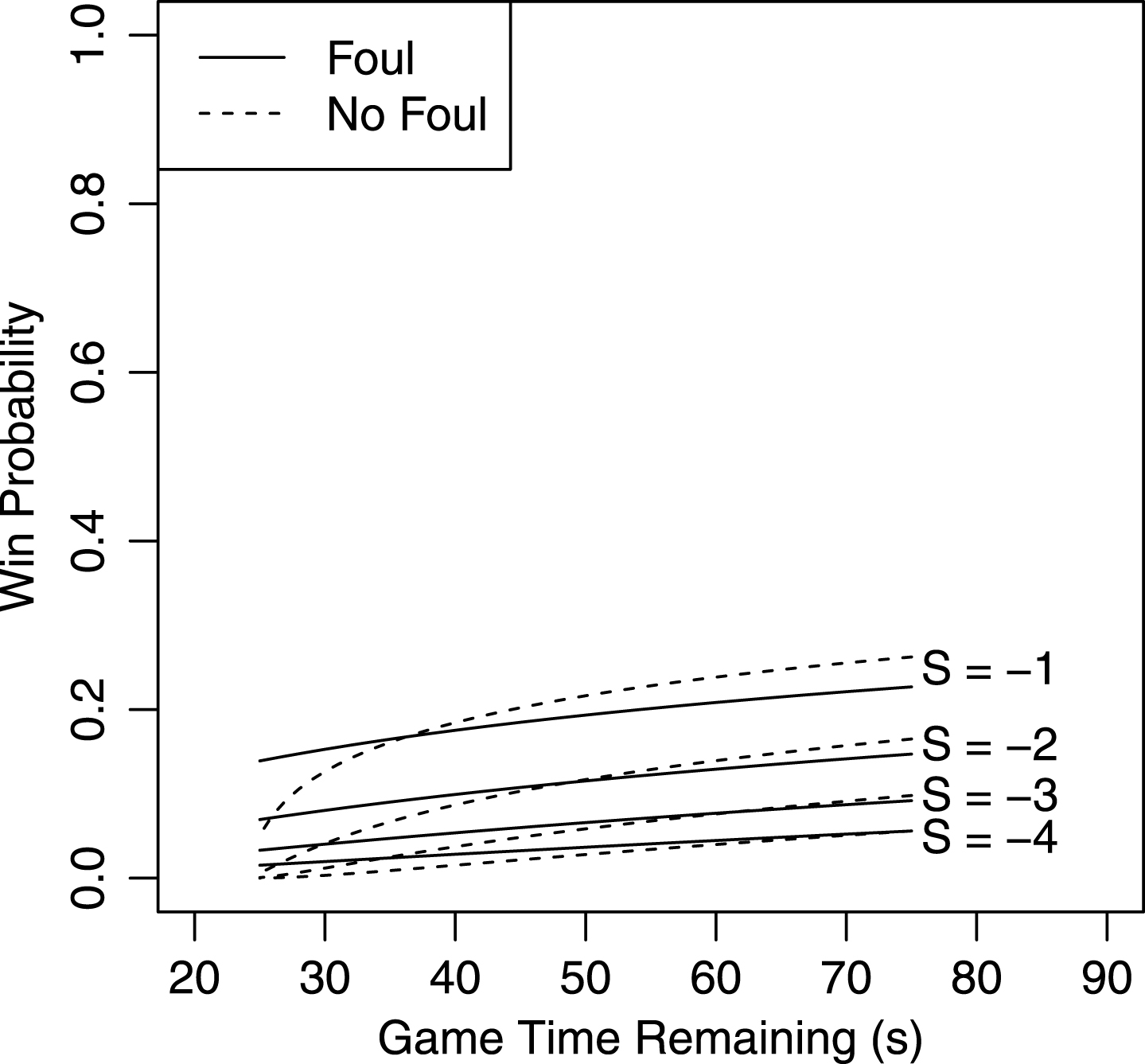
Fig. 5 shows the win probability difference between intentionally fouling and playing conventional defense for possessions beginning at a given time. The trends intuitively show that for a smaller score differential, the intentionally fouling tactic becomes optimal later in the game. For a team trailing by one through four points, intentionally fouling becomes the optimal tactic with 36, 48, 61, and 74 seconds remaining, respectively. Again, these curves will shift depending on team or player statistics used in Eq. 2. However, Fig. 5 can provide a guideline to maximize win probability when trailing late in games. This exercise also assumes a point spread of zero.
Fig.5
Win probability for different score differentials S for a team without possession. For each score differential, the win probability after deciding to intentionally foul or play conventional defense is shown.
5Conclusion
This paper details the development of an end-of-game tactics metric (ETM) to evaluate the decision-making of NBA teams at the end of close games. With a probabilistic approach to the state of an NBA game, the outcome of each NBA possession is affected by team statistics and tactical decisions made on the court. ETM judges these decisions against an optimal decision that considers all possible outcomes of a possession. ETM alone is mildly correlated with winning percentage in these close games. Using ETM and win probability, specific NBA tactics concerning intentionally fouling while both leading and trailing are studied to reveal the ideal decision-making in such situations, with the acknowledgement of the difficulty of executing such tactics. ETM can easily be expanded beyond aggregate team statistics to consider specific players, play types, or additional applications.
References
1 | Annis D., (2006) , Optimal End-Game Strategy in Basketball. Journal of Quantitative Analysis in Sports, [online] 2: (2). Available able at: http://sportsquant.com/AnnisJQAS1030.pdf [Accessed 30 Nov 2016]. |
2 | Basketball Reference, (2015) , [online] Basketball Statistics and History | Basketball-Reference.com. Available at: http://www.basketball-reference.com/ [Accessed 30 Nov 2016]. |
3 | Beuoy M., (2015) , Updated NBA Win Probability Calculator. [online] Inpredictable. Available at: http://www.inpredictable.com/ [Accessed 30 Nov 2016]. |
4 | Burke B., (2010) , Win Probability Added (WPA) Explained. [online] Advanced Football Analytics. Available at: http://archive.advancedfootballanalytics.com/2010/01/winprobability-added-wpa-explained.html [Accessed 30 Nov 2016]. |
5 | Cervone D., D’Amour A., Bornn L., and Goldsberry K., (2014) , POINTWISE: Predicting Points and Valuing Decisions in Real Time with NBA Optical Tracking Data, MIT Sloan Sports Analytics Conference. |
6 | Luo E., (2017) , [online] statsnba-playbyplay. Available at: https://www.doc.ic.ac.uk/yl11416/statsnba-data/ via http://stats.nba.com/ [Accessed 30 Aug 2017]. |
7 | NBA.com, (2015) , [online] League Team Tracking Shots. Available at: http://stats.nba.com/league/team/shots/ [Accessed 30 Nov 2016] |
8 | Sports Database, (2015) , [online] NBA Sport Data Query Language Access. Available at: http://sportsdatabase.com/ [Accessed 30 Nov 2016]. |
9 | Tango T., (2007) , The Book: Playing the percentages in baseball. Washington, D.C.: Potomac Books. |
10 | Team Rankings, (2015) , [online] NBA Team Personal Fouls Per Possession. Available at: https://www.teamrankings.com/nba/stat/personal-fouls-perpossession? date=2016-06-20 [Accessed 30 Nov 2016]. |


