
Schedule inequity in the National Basketball Association
Abstract
Scheduling factors such as a visiting team playing a game back-to-back against a rested home team can affect the win probability of the teams for that game and potentially affect teams unevenly throughout the season. This study examines schedule inequity in the National Basketball Association (NBA) for the seasons 2000–01 through 2018–19. By schedule inequity, we mean the effect of a comprehensive set of schedule factors, other than opponents, on team success and how much these effects differ across teams. We use a logistic regression model and Monte Carlo simulations to identify schedule factor variables that influence the probability of the home team winning in each game (the teams playing are control variables) and construct schedule inequity measures. We evaluate these measures for each NBA season, trends in the measures over time, and the potential effectiveness of broad prescriptive approaches to reduce schedule inequity. We find that, although schedule equity has improved over time, schedule differences disproportionately affect team success measures. Moreover, we find that balancing the frequency of schedule variables across teams is a more effective method of mitigating schedule inequity than reducing the total frequency, although combining both methods is the most effective strategy.
1Introduction
We examine a largely neglected aspect of a team’s season performance: schedule inequity. We define specific measures of schedule inequity later, but, essentially, we mean the degree to which scheduling factors (other than opponents) favor one team over another. While previous studies have analyzed the effects of individual scheduling factors such as back-to-back games, travel across time zones, and day games on game outcomes, we systematically explore the possibility that schedule differences for a comprehensive set of schedule factors over the course of a season could cause significant performance differences among teams, independent of their relative strength. Therefore, we undertake the following:
• evaluate the effects of many schedule factors (in addition to back-to-back games) on visiting and home teams and use these effects to assess cumulative effects on each team across each entire season;
• control for the teams playing each game to isolate the effects of the schedule factors;
• explore multiple measures of schedule inequity (each reflecting a different team success measure, such as the number of wins, conference rank, and probability of making the playoffs) to determine which ones are the most and least affected by schedule differences and to study the nature of the teams that are most affected for each measure;
• evaluate trends for each measure of schedule inequity over time; and
• evaluate potential benefits of broad prescriptive principles for reducing schedule inequity.
We do not examine the relative “strength of schedule,” which invariably entails an assessment of the relative quality of opponents faced by a particular team.
We start by developing a logistic regression model to assess the effect of various schedule factors on the probability that the home team in the National Basketball Association (NBA) wins. The teams (and their relative strengths) are control variables for our purposes. We are interested in the effects of the schedule factors. For example, a critical consideration is whether either team played a game the previous day (i.e., the current game is the second of a back-to-back pair of games). Each schedule factor that we identified as significant was represented by one or more variables in the model. We refer to these variables as schedule factor variables (SFVs). We first use each SFV’s model coefficient, frequency, and frequency imbalance to examine the relative SFV impact on schedule inequity. Then, we use the model coefficients to develop analytical measures of schedule inequity—how much the SFVs affect each team’s performance, and how these effects differ across teams.
In addition, we use the model coefficients in conjunction with Monte Carlo simulations of NBA seasons (including playoffs) to develop further measures of schedule inequity. Next, we assess all schedule inequity measures for each NBA season from 2000–01 to 2018–19 and evaluate trends in the measures. Finally, we alter the actual occurrences of the SFVs in each NBA season in broad, systematic ways and reconstruct all the schedule inequity measures to study the sensitivity of the measures to possible approaches to reduce schedule inequity through schedule changes. We interpret these results from the perspective of both individual teams and the league.
1.1Motivating example
Although a single numeric example is not statistically valid for assessing schedule inequity, it will provide a clear initial exposure to what we have examined. In the 2009–10 NBA season, the Charlotte Bobcats finished seventh in the Eastern Conference (hence making the playoffs), with a 44–38 record, and the Toronto Raptors finished ninth (hence missing the playoffs), with a 40–42 record. In that year, however, our analysis showed that Charlotte had an easier schedule (in terms of SFVs, not teams played) than the league average, with an estimated effect of adding 0.41 wins to their total. In comparison, Toronto played a harder-than-average schedule with an estimated effect of subtracting 0.57 wins from their total. Most importantly, since both were contending for the last playoff position, the schedule effects increased the probability of making the playoffs by .0402 for Charlotte and decreased the probability by .0717 for Toronto. The effects were mostly due to the four SFVs:1
1. Charlotte played two more games as the home team when the visiting team played back-to-back (giving them an advantage) than they did as the visiting team playing back-to-back (giving the opponent the advantage). The opposite was true for Toronto by three games.
2. Charlotte played six more games as the away team when the home team played back-to-back (giving them an advantage) than they did as the home team playing back-to-back (giving the opponent an advantage). Toronto played an equal number of each.
3. Charlotte played six more games as the visitor, where the home team played a compressed schedule of four or more games in a week2 (giving them the advantage) than as the home team playing the compressed schedule (giving the opponent the advantage). Toronto had an equal number of each.
4. Toronto played nine more home games as day games (where the home team does not do as well) than they did as the visiting team, whereas Charlotte played only one more such game.
These are statistically estimated effects and probabilities; it is difficult to predict whether a different schedule would have changed the performance or decided which teams made the playoffs. The differential effect of .1119 (.0402 + .0717) on the two teams’ probabilities of making the playoffs is substantial. However, this is just one comparison between two teams in one season. Comparing other teams in other seasons yielded different results. A contribution of this study is to assess the effects of a comprehensive set of scheduling factors on all teams across many seasons in a statistically sound manner.
1.2Literature review
There is a significant growing body of literature on the effect of scheduling factors on game outcomes. Entine and Small (2008) analyzed the differences between home and visiting teams in scheduling back-to-back games on win margins for NBA games during 2004–2006. They reported that home teams had a scoring margin advantage of 3.24 points, mostly attributable to the visiting team playing more back-to-back games (10.4%) and playing two consecutive games with more travel time (30.8%).3 Ashman et al. (2010) explored whether betting point spreads appropriately priced the negative effects of differences in fatigue and travel time on the home team’s win percentage in back-to-back situations for NBA games. During 1990–2009, they found that when both teams were playing without a day of rest, the home team win percentage against the spread was 50.63%. However, if the home team was playing without a day of rest and the visiting team was not, then the home team’s win percentage against the spread declined to 45.86%. Huyghe et al. (2018) explored the effects of frequent air travel, which can negatively affect athlete health and performance, on the home team’s win percentage. Using data for the 2010 and 2015 NBA seasons, they reported that eastward traveling teams scored more points per game and had a higher win percentage.4 Reportedly, none of these studies has examined the distribution of these factors or their cumulative differential effects across teams for an entire season. Kelly (2010) analyzed the scheduling of back-to-back NBA games during 1999–2004 and found that differences in the distribution of total occurrences might have been cumulatively significant enough to affect team rankings, although he did not quantify the likelihood. Following these studies, we are interested in the effect of these (and other) schedule factors on game outcomes. Similar to Kelly (2010), we are also interested in whether the distribution of schedule factors across a season potentially affects team performance inequitably. We systematically examined all significant factors and their relative effects, considering how often each team was placed in an advantageous or disadvantageous situation based on their schedule and their opponents’ schedule. We observe that the opponent’s schedule factors are equally important to those of the team itself. The ultimate contribution of our study is this systematic look at schedule inequity, which is comprehensive in both its examination of schedule factors and their distribution across teams.
An area of research closely related to schedule inequity is sports timetabling, which deals with approaches to alter schedules so that the distribution of one or more scheduling factors is evenly balanced. Goossens et al. (2020) showed that adding a constraint for fairness in an adverse scheduling factor distribution can increase the total occurrence of adverse factors. Yang (2017) showed that, for the NBA, reducing occurrences of back-to-back games (favorable to players) reduces total travel time but spreads games more evenly between weekdays and weekends (unfavorable to team owners and TV broadcasters). These considerations have led to the development of a software to make and remake schedules with a quick turnaround time.5
Although we do not attempt to develop a scheduling algorithm that would directly contribute to the sports timetabling literature, we present the results of some broad-based approaches to alter the frequency and distribution of schedule factors that should help guide future research in this area. It should be noted that any attempt to manipulate a schedule factor without considering other factors (including those faced by both teams) in a game will not achieve its presumed objective.
Our method for evaluating each team’s total advantage or disadvantage across a season is to compare its performance using the actual schedule to the benchmark of a “reference” schedule where each game will be played with each team having played 2 days ago and no other factors that might give one team an advantage over the other being present.6 We note that this reference schedule can never be achieved in reality but allows each team to be compared to the other team and schedule inequities to be assessed by virtue of each team being compared to the same reference schedule.
Schedule inequity is an important subject because, to the extent that schedule imbalances materially affect season-long performance, we think most people (team owners, fans, and other stakeholders) would consider this counter to the fundamentals of fair competition. Teams commit a great deal of money and other resources to achieve success. Schedule inequity could affect this success and, importantly, could have a substantial economic impact on potential arena attendance and broadcast and other revenue. While our results show that schedule differences may be of little consequence for some teams (particularly high- or low-quality teams), these differences are significant for many others. We show, for example, that over the 2000–01 through the 2018–19 NBA seasons, differences attributable solely to scheduling imbalances between the most favorably affected and most disadvantaged teams averaged 1.87 expected wins per season. We emphasize that this is the average difference in expected wins after controlling for team quality and represents the impact of scheduling differences alone. Further, we calculated an average difference of .0825 (or 8.25%) between the effects on the probability of making the playoffs for the most positive and most negative “schedule-affected” teams.
To illustrate the potential economic impact of schedule inequity, Schaefer (2020) states that “the NBA makes an average of $1.2 million in gate revenue per regular-season game and $2.0 million for each playoff game.” In addition, Gough (2020) lists the total revenue for each NBA team for the 2018–19 season. The New York Knicks had $472 million, while the New Orleans Pelicans had $224 million in total (i.e., gate and broadcast) revenue. The median team’s total revenue was approximately $285 million. Missing the eighth playoff spot solely due to schedule inequity costs a team a minimum of $4 million in gate revenue (two missed playoff home games) and at least as large a loss in broadcast revenue. This is a substantial reduction in season revenue for the adversely affected teams. The ability to measure schedule inequity is likely to be even more critical when schedules are altered significantly for reasons such as the COVID-19 pandemic, lockouts, or even new ideas, such as in-season tournaments. To illustrate, Baker (2020) reported that less travel (a consequence of the NBA’s “bubble” environment developed in response to COVID-19) contributed to higher quality basketball. He further noted that “(d)uring the 2018–2019 season, NBA teams traveled an average of 43,534 miles, nearly 7% more than NHL teams (40,768), 36% more than MLB teams (31,993), and 441% more than NFL teams (18,049).”
The remainder of this article is organized as follows: Section 2 describes the process used to compute relevant measures of schedule inequity. Section 3 presents and discusses our results, including an evaluation of ways to mitigate the impact of schedule inequity. Finally, Section 4 presents concluding remarks.
2Model development and methodology
2.1Overview of our process
We first developed a logistic regression model to assess the effect of various scheduling factors on the probability that the home team in NBA games wins the game. We used the model coefficients and frequency of measures for each variable in the model to assess the relative impact of the SFVs. We then used the model coefficients to develop measures of schedule inequity. By inequity, we mean the extent to which the SFVs’ effects on performance differ across teams. We initially developed analytical measures and then utilized Monte Carlo simulations of NBA seasons (including playoffs) to develop further measures that could not be obtained analytically. We estimated all scheduling inequity measures for each NBA season from 2000–01 to 2018–19, examining trends in the measures over the 19 years. Finally, we sequentially altered the schedules to examine the relative effectiveness of broad principles for reducing schedule inequity.
2.2Logistic regression
We used data from basketball-reference.com for the 2000–01 through 2018–19 NBA seasons. This period was chosen for two reasons. First, prior to the 2000–01 season, the start time of games was not included in the data, and we wanted to look at possible effects that involve time. Second, we wanted relatively recent data to keep factors not available (e.g., travel modes, accommodations, nutrition) somewhat consistent while still allowing for sufficient data to evaluate a variety of schedule variables.
Determining which factors to include in any logistic regression model is often difficult. In the case of scheduling inequity, the literature has identified various factors that affect game outcomes, but there are many possibilities for quantifying various factors. For example, prior studies (Ashman et al., 2010; Entine & Small, 2008; Huyghe et al., 2018) have shown that travel can adversely affect a team’s chances of winning. Is this effect primarily due to length of travel, the mere fact that travel is involved, travel across time zones, cumulative travel over some time period, or just travel from the previous game?
Prior studies (e.g., Kelly, 2010; Entine & Small, 2008) clearly show that playing games on consecutive dates hurts a team’s chances of winning the second game. We started our model development with this observation extended to the categorical variable “number of days since the previous game.” We chose the value “two” as the reference category as this is the most common time between games and closest to the average. The other possibilities were mostly left as individual categories except for large values, which needed some grouping due to lack of frequency. This last grouping was determined by identifying when the increase in the number of days between games hurts the team’s chances. The categories derived were used as the baseline model.
Table 1
Logistic regression results
| Number | Description | Odds multiplier | p-value Wald chi sq |
| Reference category for variables 1–12 is 2 days since the previous game. | |||
| SFV1 | Open at home | 1.123 | 0.6471 |
| SFV2 | Home 1 day since last game | 0.806 | <0.0001 |
| SFV3 | Home 3 days since last game | 0.988 | 0.7811 |
| SFV4 | Home 4 days since last game | 0.967 | 0.6476 |
| SFV5 | Home 5 days since last game | 1.213 | 0.2602 |
| SFV6 | Home>5 days since last game | 0.812 | 0.2246 |
| SFV7 | Open as the visiting team | 1.182 | 0.5454 |
| SFV8 | Visitor 1 day since last game | 1.506 | <0.0001 |
| SFV9 | Visitor 3 days since last game | 0.992 | 0.8695 |
| SFV10 | Visitor 4 days since last game | 0.984 | 0.8616 |
| SFV11 | Visitor 5 or 6 days since last game | 0.771 | 0.1176 |
| SFV12 | Vis.>6 days since last game | 1.741 | 0.0315 |
| SFV13 | Visitor played> =3 games in the last week (not a back-to-back game) | 1.153 | 0.0053 |
| SFV14 | Visitor travel > 1000 miles if back-to-back or > 2000 miles if not | 1.261 | 0.0043 |
| SFV15 | Home played> =4 games in last week (not a back-to-back game) | 0.914 | 0.0112 |
| SFV16 | Home travel at least 1 time zone W to E from game 1 day ago | 0.693 | 0.0013 |
| SFV17 | Home travel at least 2 time zones W to E from game 2 days ago | 0.833 | 0.1092 |
| SFV18 | Day game (2 pm or earlier) | 0.904 | 0.2037 |
| SFV19 | Visitor back-to-back following a 1 game home stand | 1.090 | 0.2449 |
| SFV20 | Visitor first game of a set of back-to-back games | 1.055 | 0.1588 |
We then conducted exploratory investigations into many other possible factors by comparing model predictions with actual results. For example, to examine the effect of playing many games in a compressed time frame, the percentage of actual home team wins versus the predicted percentage from the baseline model was computed for various games in various periods. We tried several potential methods and chose the best based on the significance of the variable (p-value for the Wald Chi-square test) and the amount and consistency of the increase in the receiver operating characteristic (ROC) curve area, using 10-fold cross-validation. Across many factors and ways of quantifying each factor, we added variables to the baseline model based on the cross-validation results until it was not helpful to add further variables.
2.3The final logistic regression model
The dependent variable was whether the home team won the game. The control variables were a series of dummy variables identifying which teams were the home and visiting teams.7 The schedule-related variables included in the final model are shown in Table 1, along with the odds multiplier estimates and p-values.
The first 12 SFVs are categorical variables for the number of days since the previous game for the home team and the visiting team or whether this was the opener for the home or visiting team; the reference category was 2 days since the previous game for both the home and visiting team variables. Some of these variables were not significantly different from the 2-day reference but were included for insight into the period of rest that is long enough to switch from being helpful to harmful. Odds multipliers less than 1 disadvantage the home team expected win probability and values greater than 1 advantage the home team. Comparing back-to-back games shows that the home team (SFV2 = 0.86) is disadvantaged when playing back-to-back but not as much as it is advantaged when the visiting team is playing back-to-back (SFV8 = 1.506). The effects of a compressed schedule were captured using SFV13 and SFV15. A home team playing a compressed schedule is disadvantaged (SFV15 = 0.914) but slightly more advantaged if the visiting team plays a compressed schedule (SFV13 = 1.153). The home team would be advantaged if the visiting team traveled a considerable distance from their previous game (SFV14 = 1.261). SFV16 and SFV17 show the effects of home team travel across time zones. As expected, travel across at least two time zones in 2 days disadvantages the home team (SFV17 = 0.833) less than crossing time zones in 1 day (SFV16 = 0.693) due to the rest day. Some of the p-values for the remaining variables SFV18–SFV20 were, perhaps, not impressively low, but all variables consistently led to increases in the ROC curve8 areas in cross-validation testing and are intuitively reasonable.9
The logistic regression model evaluates which factors affect individual game outcomes, but it does not directly assess schedule inequity. This requires analyzing the effects of the SFVs on individual teams’ performances across an entire season, which is our primary contribution, and the remaining study describes both our methodology and the results. However, before conducting the analysis, we wanted to construct some broad-based measures to assess the relative impact of each SFV on schedule inequity.
Table 2
Logistics regression model: Variable impacts
| (1) Schedule factor variable number | (2) Average effect | (3) Total occurrences | (4) Impact (2) x (3) x 2 | (5) Percent of impact | (6) Games imbalance | (7) Impact & imbalance (2) x (6) | (8) Percent of impact & imbalance |
| SFV1 | 0.0217 | 306 | 13.3 | 0.5 | 544 | 11.8 | 2.1 |
| SFV2* | 0.0412 | 3466 | 285.3 | 9.7 | 1448 | 59.6 | 10.7 |
| SFV3 | 0.0023 | 3904 | 17.7 | 0.6 | 1626 | 3.7 | 0.7 |
| SFV4 | 0.0064 | 1065 | 13.7 | 0.5 | 758 | 4.9 | 0.9 |
| SFV5 | 0.0352 | 204 | 14.4 | 0.5 | 266 | 9.4 | 1.7 |
| SFV6 | 0.0396 | 330 | 26.1 | 0.9 | 540 | 21.4 | 3.9 |
| SFV7* | 0.0315 | 260 | 16.4 | 0.6 | 486 | 15.3 | 2.8 |
| SFV8 | 0.0774 | 7251 | 1121.9 | 38.3 | 1938 | 149.9 | 27.0 |
| SFV9 | 0.0014 | 2966 | 8.6 | 0.3 | 1382 | 2.0 | 0.4 |
| SFV10 | 0.0031 | 627 | 3.9 | 0.1 | 606 | 1.9 | 0.3 |
| SFV11 | 0.0509 | 264 | 26.9 | 0.9 | 388 | 19.8 | 3.6 |
| SFV12 | 0.1097 | 118 | 25.9 | 0.9 | 216 | 23.7 | 4.3 |
| SFV13 | 0.0272 | 12881 | 701.9 | 24.0 | 1974 | 53.8 | 9.7 |
| SFV14 | 0.0434 | 891 | 77.3 | 2.6 | 618 | 26.8 | 4.8 |
| SFV15 | 0.0170 | 7462 | 253.5 | 8.6 | 1828 | 31.0 | 5.6 |
| SFV16 | 0.0706 | 500 | 70.6 | 2.4 | 652 | 46.0 | 8.3 |
| SFV17 | 0.0340 | 451 | 30.7 | 1.0 | 540 | 18.4 | 3.3 |
| SFV18 | 0.0204 | 939 | 38.3 | 1.3 | 962 | 19.6 | 3.5 |
| SFV19 | 0.0160 | 1299 | 41.7 | 1.4 | 962 | 15.4 | 2.8 |
| SFV20 | 0.0102 | 7004 | 142.7 | 4.9 | 1976 | 20.1 | 3.6 |
*Back-to-back.
We construct two measures of this kind and present them in Table 2. The first measure (hereafter referred to as the impact measure [Column 4]) was obtained by multiplying the frequency (Column 3) by the average effect (Column 2). The impact measure captures the frequency and magnitude but ignores the possibility that factor occurrences are distributed unevenly across the teams. The second measure (hereafter referred to as the impact and imbalance measure [Column 7]) was computed by multiplying the imbalance of each factor’s occurrences (absolute value of the difference between home and away occurrences [Column 6]) for each team by the average effect (Column 2) and summing across all teams. The relative impact results are shown in Table 2 for both measurement methods, along with the percentage contribution of each of the SFVs (Columns 5 and 8, respectively).
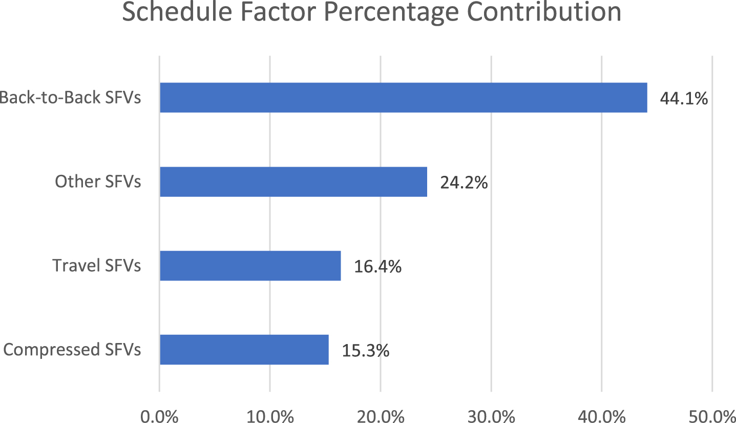
The visiting team playing a back-to-back game (SFV8) makes the largest contribution to both the impact measure (38.3%) and the impact and imbalance measure (27%). The home team playing a back-to-back game (SFV2) has the third highest impact on the impact measure (9.7%) and the second most impact for the impact and imbalance measure (10.7%), but this is less than half the impact of the visiting team playing back-to-back as both the effect on each game and the frequency are much lower. The visiting team playing a compressed schedule of three or more games in a week (SFV13) makes the second largest contribution to the impact measure (24%) and the third largest to the impact and imbalance measure (9.7%). Looking at the impact and imbalance measure, as shown in Fig. 1, we see that the back-to-back variables (SFVs 2, 8, 19, 20), travel variables (SFVs 14, 16, 17), and compressed schedule variables (SFVs 13, 15) account for 44.1%, 16.4%, and 15.3% of the total imbalance, respectively. Furthermore, the imbalance and impact measure shows that the total scheduling effects on the visiting team are larger (59.3%) than on the home team (40.7%). This is consistent with our earlier observation that the schedule factor of back-to-back games has more effect when it is the visiting team than when it is the home team, as well as the fact that more SFVs are associated with the visiting team than with the home team. In addition, it seems intuitive that schedule factors would compound the natural fatigue from being on the road.
Fig. 1
Impact and imbalance measure: SFVs’ % contributions. Other SFVs are as follows: Visitor travel > 1000 miles if back-to-back or > 2000 miles if not (SFV 14), Home travel at least 1 time zone W to E from game 1 day ago (SFV 16), Home travel at least 2 time zones W to E from game 2 days ago (SFV 17).
2.4Measures of schedule inequity
Each measure of schedule inequity is based on some characterization of team success across an entire season. For example, the first measure we developed is based on the expected value of the number of wins. The first step for each measure was to estimate each team’s team success value in two different ways:
a) Using the actual schedule
b) Using the reference “22 schedule”
Subtracting b) from a) yields a measure of the scheduling effects on that team. A negative (positive) value indicates that the team’s schedule was more disadvantageous (advantageous) than the reference 22 schedule. Since each negative effect on one team has a positive effect on the opponent, the sum of effects across all teams is always 0. Although our expository example compared two specific teams (Charlotte and Toronto), comparing each team to the reference 22 schedule avoids the need to make every possible pairwise team comparison.
The first characterization of team success was the expected value of the number of wins. This is an analytical characterization that was computed by summing the home team win probabilities (the model predicted values) across all home games for a team in a season and the visiting team win probabilities (1 –the model predicted values) across all the visiting games for that team in the same season.
This first measure of the effect of the schedule on team success reflects the fact that each SFV has a larger effect on a team’s probability of winning if the game is expected to be competitive. This means that the cumulative effects tend to be lower for the highest quality and lowest quality teams because they play less competitive games on average. Also, as aforementioned, the SFVs have a more significant overall impact on the visiting team than the home team. This means that good (but not the best) teams tend to get hurt the most by the schedule factors because their visiting games are more competitive than their home games. Conversely, weak (but not the worst) teams tend to benefit the most.
Our second measure of the effect of the schedule on team success is also based on using the expected number of wins as the team success characterization but with an important change: it depends not on the quality of the teams but only on the schedule itself. To construct such a measure, we first computed the effect of each factor on the probability of a home team winning each game in which that factor was present (by subtracting the win probability with the factor from the win probability without the factor) and averaged across all such games. We then re-computed part a) using the average (rather than the actual) effect of each SFV on every game it was present. Part b) did not change; therefore, the result is the estimated effect of the schedule on the expected number of wins for each team (compared to the 22 schedule) if the effects of each factor on each game were the same (the average effect value), independent of the teams playing. Two teams with the same schedule (SFVs present the same number of times) have the same estimated effect with this approach, regardless of the teams’ quality.
The first two measures of the effect of the schedule on team success were obtained analytically:
1. Expected number of wins
2. Expected number of wins using the average SFV effects
The remaining measures required the use of Monte Carlo simulation. These simulation-based measures were obtained for five additional characterizations of team success:
3. Probability of being NBA champion
4. Probability of being conference champion
5. Probability of making the playoffs
6. League rank
7. Conference rank
Table 3
Individual team measures 2009–10
| Team | Expected wins | Expected wins (Avg. var. effect) | League champ. prob. | Conf. champ. prob. | Playoff prob. | League rank | Conference rank |
| Atlanta | –0.7885 | –0.1590 | –0.0018 | –0.0044 | 0.0000 | 0.3206 | 0.1670 |
| Boston | –0.2229 | –0.2140 | –0.0004 | –0.0006 | 0.0000 | 0.0702 | 0.0710 |
| Charlotte | 0.5158 | 0.4090 | 0.0001 | 0.0001 | 0.0402 | –0.3677 | –0.1180 |
| Chicago | 0.3055 | 0.2640 | 0.0001 | 0.0000 | 0.0188 | –0.0940 | –0.0021 |
| Cleveland | –0.1046 | 0.4180 | 0.0037 | 0.0046 | 0.0000 | –0.1142 | –0.0459 |
| Dallas | –0.2131 | –0.2550 | 0.0011 | 0.0017 | –0.0023 | –0.1912 | –0.1817 |
| Denver | –0.3478 | –0.0350 | –0.0005 | 0.0009 | 0.0036 | 0.1057 | 0.0251 |
| Detroit | 0.2093 | –0.1260 | 0.0000 | 0.0000 | –0.0012 | 0.0310 | –0.0470 |
| Golden State | 0.3947 | –0.1110 | 0.0000 | 0.0000 | 0.0000 | –0.0432 | 0.0449 |
| Houston | –0.1993 | –0.1750 | 0.0000 | 0.0002 | –0.0035 | 0.2024 | 0.0230 |
| Indiana | –0.2330 | –0.5060 | 0.0000 | 0.0000 | –0.0129 | 0.2253 | 0.1169 |
| LA Clippers | 0.8159 | 0.3710 | 0.0000 | 0.0000 | 0.0000 | –0.2710 | –0.0647 |
| LA Lakers | –1.0571 | –0.5200 | –0.0037 | –0.0046 | 0.0000 | 0.4165 | 0.2276 |
| Memphis | 0.0406 | –0.0450 | 0.0000 | 0.0001 | 0.0071 | 0.1638 | 0.0418 |
| Miami Heat | 0.6701 | 0.6250 | 0.0004 | 0.0001 | 0.0083 | –0.5868 | –0.2088 |
| Milwaukee | 0.7326 | 0.6140 | 0.0001 | 0.0005 | 0.0188 | –0.5184 | –0.1785 |
| Minnesota | 0.5653 | 0.2630 | 0.0000 | 0.0000 | 0.0000 | –0.0334 | –0.0021 |
| New Jersey | 0.1577 | –0.1710 | 0.0000 | 0.0000 | 0.0000 | 0.0267 | 0.0000 |
| New Orleans | 0.2247 | 0.1130 | 0.0000 | 0.0000 | 0.0070 | –0.0648 | –0.0480 |
| New York | 0.2475 | –0.1470 | 0.0000 | 0.0000 | 0.0035 | 0.0144 | –0.0303 |
| Oklahoma City | –0.2311 | –0.1790 | –0.0004 | –0.0001 | 0.0023 | 0.0277 | –0.0480 |
| Orlando | –0.3895 | 0.1190 | 0.0006 | 0.0002 | 0.0000 | –0.0164 | 0.0271 |
| Philadelphia | –0.2437 | –0.0420 | 0.0000 | 0.0000 | –0.0012 | 0.2374 | 0.0783 |
| Phoenix | –0.1120 | 0.1890 | 0.0010 | 0.0032 | –0.0047 | –0.0913 | –0.0532 |
| Portland | –0.4159 | –0.3000 | –0.0002 | –0.0008 | –0.0129 | 0.1869 | 0.0647 |
| Sacramento | 0.5640 | –0.0080 | 0.0000 | 0.0000 | 0.0000 | –0.1098 | –0.0052 |
| San Antonio | 0.1591 | 0.4550 | 0.0004 | 0.0008 | 0.0140 | –0.3186 | –0.2538 |
| Toronto | –0.5509 | –0.5670 | 0.0000 | –0.0001 | –0.0717 | 0.3994 | 0.2410 |
| Utah | –0.8119 | –0.3260 | –0.0004 | –0.0015 | –0.0105 | 0.4207 | 0.2330 |
| Washington | 0.3184 | 0.0430 | 0.0000 | 0.0000 | 0.0000 | –0.0355 | –0.0835 |
Similar to the analytical measures, we simulated each season in two different ways. We began by simulating the seasons using the predicted win probabilities for each game from the model using the actual schedule for the season. Next, we simulated the reference 22 schedule. Finally, we estimated the effects of the SFVs by subtracting the team success measure simulated with the actual schedule from that based on the reference 22 schedule. We simulated each season 1000 times to estimate measures 5, 6, and 7 and, for each simulated regular season, we simulated (starting with the playoff seeds from the regular-season simulations) the playoffs 100 times and used the 100 playoff simulations from each of the 1000 regular-season simulations to estimate measures 3 and 4.
The simulations of both the regular seasons and the playoffs essentially consist of simulating which team wins each game and keeping track of the results. To simulate which team wins each game, the probability that the home team wins (from the statistical model applied to the SFVs present in that game) is compared to a random number (a value randomly generated from the probability distribution that is uniform between 0 and 1). If the home team win probability exceeds the random number, the home team wins that simulated game. If not, the visiting team wins.
We present the results for an example season as the results for each team for each season cannot be demonstrated due to space considerations. Table 3 shows the seven measures for each team for the 2009–10 season. This season corresponds to the season of our Charlotte-Toronto example and the reader can find the values referenced in that example in this table and note that among all teams Charlotte’s playoff probabilities are the most positively affected and Toronto’s are the most negatively affected.
Although it was convenient to compare any two teams using the table (as we did in our example), we wanted summary measures to characterize the level of schedule inequity across the entire league for each season. Therefore, once the effects on each team were computed for each success characterization, two summary measures of schedule inequity were computed for each season for each of the seven team success measures. The first summary measure was obtained by computing the average absolute value of the effects on individual teams. The second measure was computed by subtracting the effect on the most disadvantaged team (the most negative value) from the effect on the most advantaged team (the most positive value). For ease of exposition in the remaining study, we refer to the average absolute value and range of effects using AAV1 and RE1 for the first team success measure, AAV2 and RE2 for the second team success measure, and so on. For example, for 2009–10, AAV1 is the average of the absolute values of the numbers in Column 1 of Table 3 and RE1 is the most negative value in Column 1 subtracted from the most positive value in Column 1 of Table 3. Similarly, for 2009–10, AAV2-AAV6 and RE2-RE6 are obtained in the same manner using Columns 2–6 of Table 3.
Table 4
Average absolute value (AAV) results by NBA season
| Expected wins AAV1 | Expected wins (Avg. var. effect) AAV2 | League champ. prob. AAV3 | Conf. champ. prob. AAV4 | Playoff prob. AAV5 | League rank AAV6 | Conference rank AAV7 | |
| 2000 | 0.3744 | 0.1964 | 0.00024 | 0.00063 | 0.00489 | 0.1449 | 0.0694 |
| 2001 | 0.4141 | 0.1997 | 0.00030 | 0.00067 | 0.00895 | 0.1744 | 0.0947 |
| 2002 | 0.3517 | 0.2124 | 0.00036 | 0.00075 | 0.00787 | 0.1450 | 0.0756 |
| 2003 | 0.4590 | 0.2774 | 0.00032 | 0.00070 | 0.01215 | 0.2035 | 0.1106 |
| 2004 | 0.3578 | 0.2024 | 0.00106 | 0.00111 | 0.00889 | 0.1733 | 0.0880 |
| 2005 | 0.4742 | 0.2827 | 0.00029 | 0.00035 | 0.01593 | 0.2298 | 0.1179 |
| 2006 | 0.3334 | 0.2472 | 0.00013 | 0.00066 | 0.01342 | 0.2353 | 0.1202 |
| 2007 | 0.3589 | 0.2453 | 0.00035 | 0.00095 | 0.00798 | 0.1868 | 0.1087 |
| 2008 | 0.3742 | 0.2447 | 0.00047 | 0.00077 | 0.00943 | 0.1666 | 0.1120 |
| 2009 | 0.3948 | 0.2590 | 0.00048 | 0.00080 | 0.00825 | 0.1902 | 0.0911 |
| 2010 | 0.3581 | 0.2306 | 0.00030 | 0.00036 | 0.00761 | 0.1399 | 0.0721 |
| 2011 | 0.2604 | 0.1792 | 0.00027 | 0.00058 | 0.00523 | 0.1506 | 0.0723 |
| 2012 | 0.4550 | 0.1886 | 0.00054 | 0.00143 | 0.00689 | 0.1696 | 0.0930 |
| 2013 | 0.3160 | 0.2183 | 0.00038 | 0.00062 | 0.00677 | 0.1745 | 0.0893 |
| 2014 | 0.3580 | 0.2235 | 0.00007 | 0.00026 | 0.00953 | 0.1629 | 0.0748 |
| 2015 | 0.3688 | 0.2039 | 0.00040 | 0.00067 | 0.00723 | 0.1458 | 0.0736 |
| 2016 | 0.2601 | 0.1764 | 0.00005 | 0.00022 | 0.00710 | 0.1276 | 0.0619 |
| 2017 | 0.2606 | 0.1810 | 0.00009 | 0.00022 | 0.00613 | 0.1606 | 0.0766 |
| 2018 | 0.2993 | 0.1701 | 0.00024 | 0.00053 | 0.00683 | 0.1659 | 0.0867 |
| Avg. | 0.3627 | 0.2178 | 0.00033 | 0.00065 | 0.00848 | 0.1709 | 0.0889 |
Table 5
Range of effects results by NBA season
| Expected wins RE1 | Expected wins (Avg. var. effect) RE2 | League champ. prob. RE3 | Conf. champ. prob. RE4 | Playoff prob. RE5 | League rank RE6 | Conference rank RE7 | |
| 2000 | 2.1370 | 1.1770 | 0.0024 | 0.0074 | 0.0433 | 1.1921 | 0.5206 |
| 2001 | 1.7750 | 1.1850 | 0.0042 | 0.0058 | 0.0751 | 1.0520 | 0.5604 |
| 2002 | 1.8310 | 0.9440 | 0.0059 | 0.0084 | 0.0751 | 0.7113 | 0.3694 |
| 2003 | 1.8990 | 1.2150 | 0.0046 | 0.0094 | 0.1133 | 1.1151 | 0.5754 |
| 2004 | 1.8740 | 1.3320 | 0.0269 | 0.0240 | 0.0906 | 1.1074 | 0.5295 |
| 2005 | 2.1950 | 1.5840 | 0.0068 | 0.0061 | 0.1501 | 1.7127 | 0.8173 |
| 2006 | 1.9180 | 1.3690 | 0.0020 | 0.0109 | 0.1281 | 1.4467 | 0.7672 |
| 2007 | 2.1780 | 1.2970 | 0.0060 | 0.0164 | 0.0711 | 0.9841 | 0.5940 |
| 2008 | 2.2570 | 1.0360 | 0.0117 | 0.0138 | 0.0844 | 0.8189 | 0.6344 |
| 2009 | 1.8730 | 1.1920 | 0.0074 | 0.0092 | 0.1119 | 1.0075 | 0.4948 |
| 2010 | 1.8760 | 1.1750 | 0.0067 | 0.0056 | 0.0749 | 0.9824 | 0.4558 |
| 2011 | 1.5480 | 0.9340 | 0.0057 | 0.0111 | 0.0541 | 0.7015 | 0.3773 |
| 2012 | 2.0090 | 0.9660 | 0.0123 | 0.0298 | 0.0734 | 0.9353 | 0.4923 |
| 2013 | 1.8100 | 1.2070 | 0.0045 | 0.0073 | 0.0727 | 0.8537 | 0.4108 |
| 2014 | 1.8060 | 0.9290 | 0.0008 | 0.0042 | 0.0928 | 0.8787 | 0.5277 |
| 2015 | 2.2370 | 1.1250 | 0.0118 | 0.0124 | 0.0618 | 0.8442 | 0.5220 |
| 2016 | 1.3050 | 0.8670 | 0.0007 | 0.0021 | 0.0649 | 0.7008 | 0.3204 |
| 2017 | 1.5550 | 1.0500 | 0.0009 | 0.0021 | 0.0612 | 0.9483 | 0.5312 |
| 2018 | 1.4730 | 1.0040 | 0.0023 | 0.0049 | 0.0697 | 0.8223 | 0.4550 |
| Avg. | 1.8714 | 1.1362 | 0.0065 | 0.0100 | 0.0825 | 0.9903 | 0.5240 |
3Results
3.1Measures of schedule inequity: Numerical results
Table 4 shows the average absolute values for all measures (AAV1-AAV7) for each season. The range results (RE1-RE7) are provided in Table 5.
The average effects on wins (AAV1-AAV2) and ranks (AAV6-AAV7) seem relatively modest. The corresponding range effects (RE1-RE2 and RE6-RE7) were substantial. This indicates that individual game advantages and disadvantages largely cancel each other out for many teams, but some teams are significantly advantaged or disadvantaged each year. Although we think that a range of effects on expected wins between one and two games in a season due to schedule factors is significant—given how valuable a win or two can be sometimes—it is probably easier to judge the significance of the effects by looking at the probability-based measures for league champion, conference champion, and making the playoffs (AAV3-AAV5 and RE3-E5). It should be noted that, for all three probability-based measures, the effect on most teams each year is close to 0, affecting AAV3-AAV5. Only the highest quality teams have a significant chance of winning the league or conference championships; these teams also play less competitive games on average, so individual game effects are generally smaller. Thus, it is not surprising that AAV3 and AAV4 are small. It is encouraging that the ranges of effects RE3 and RE4 are modest, although much larger than the corresponding average absolute value effects. Although the ranges of effects are not negligible, it does seem that schedule inequities do not play a significant role in deciding who wins it all.
Table 6
Distribution of team values summary measures
| Expected wins RE1 | Expected wins (Avg. var. effect) RE2 | League champ. prob. RE3 | Conf. champ. prob. RE4 | Playoff prob. RE5 | League rank RE6 | Conference rank RE7 | |
| Std. dev./AAV | 1.255 | 1.274 | 2.461 | 2.214 | 1.779 | 1.330 | 1.342 |
| IQR/range | .332 | .329 | .017 | .023 | .071 | .266 | 0.267 |
| % zero values | 0 | 0.3 | 36.3 | 29.6 | 32.0 | 0 | 0.4 |
Table 7
Average conference rank of most affected teams
| Average division rank of team affected most: | Wins | League champ. prob. | Conf. champ. prob. | Playoff prob. | League rank | Conference rank |
| Negatively | 3.4 | 2.6 | 2.9 | 7.8 | 7.3 | 7.3 |
| Positively | 12.4 | 2.5 | 2.7 | 8.2 | 6.1 | 6.1 |
The effects on the probability of making the playoffs (AAV5 and RE5) are the most interesting and significant measures. In our expository example, we saw that the schedule effects increased the probability of making the playoffs by .0402 for Charlotte and decreased the probability by .0717 for Toronto in 2009–10. The absolute value of each of these measures was included in the computation of the AAV5 value of .00825 for that season. We can see that the values of both teams are much larger than the average. As noted, the reason is that the average includes a lot of near-zero values since high-quality teams make the playoffs regardless of schedule inequities and low-quality teams do not—it is mostly the teams in contention for the last playoff position that are affected.
Note that this is the case not only because making the playoffs or not can often be affected due to a win or two but also because the teams that are contending for the last playoff spot play more competitive games on average than very high- or low-quality teams, so schedule effects are larger on more of the games they play. The RE5 value for the 2009–10 season is .1119, which comes from Charlotte and Toronto since they were the teams most advantaged and disadvantaged in that season. The average value of RE5 across all seasons (last row, Table 4) was .0825. This implied that, on average, across all the years we considered, the percentage chance of two teams making the playoffs was affected by an 8.25% differential solely by scheduling factors unrelated to the teams they played. This is especially significant considering the importance of making the playoffs from competitive and economic viewpoints.
The construction of schedule inequity measures AAV1-AAV7 and RE1-RE7 is the schedule inequity season summary measures we recommend and have focused on. However, as noted and observed for the example season 2009–10 in Table 3, some teams were affected marginally or nonsignificantly, whereas others were significantly affected either positively or negatively. We explored these observations with some further analysis to assess the spread of the team measures and the characteristics of the most affected teams.
Note that the average value of the individual team measures across all teams is 0 for all measures since what benefits one team hurts their opponent by the same amount. Thus, AAV1-AAV7 are the same as the mean absolute deviation (MAD) (a widely used measure of spread) for each team measure. Moreover, the range measures RE1-RE7 are the obvious measures of spread, although, similar to AAV1-AAV7, we view them mostly from the standpoint of inequity in the sense that any team affected by the schedule much more negatively than any other team is a strong indication of inequity. For additional insights into the spread of effects beyond MAD and range, Table 6 shows the (average across all seasons) standard deviation, in terms of its ratio to the MAD and the interquartile range (IQR), in terms of its ratio to the range, and the percent of team values that were 0. We have presented ratios for ease of comparison to the well-known normal distribution (bell curve). The standard deviation to MAD ratio of the normal distribution is 1.255. Although the normal distribution has an infinite range, we can compare with the IQR to total range ratios of .320 and .224 for the normal distribution truncated at 2 and 3 standard deviations, respectively, and to the ratio of .5 for the uniform distribution (evenly distributed across the entire range). Furthermore, the table shows the percent of team values that were 0 for each measure. The results for all the probability-based measures show a significant percent of 0 values that drives small IQRs (compared to the full range) and the large values for some teams lead to large standard deviations (compared to the MAD) with values in both cases very different from the bell curve. For the win-based measures, both spread summary metrics are very similar to those for the bell curve and the metrics for the rank-based measures indicate a somewhat narrower IQR compared to the range that leads to slightly higher standard deviation to MAD ratios.
Table 7 characterizes which teams were most affected by the schedule for each measure.
Table 8
Scheduling inequity trend results (excluding the 2011–12 season)
| Expected wins (1) | Expected wins (Avg. var. effect) (2) | League champ. prob. (3) | Conf. champ. prob (4) | Playoff prob. (5) | League rank (6) | Conference rank (7) | |
| Average absolute | –.0059 (.014) | –.0026 (.064) | –.000012 (.220) | –.000018 (.173) | –.00017 (.156) | –.0016 (.194) | –.0011 (.131) |
| value | |||||||
| Range of | –.0211 (.052) | –.0152 (.041) | –.00024 (.389) | –.00024 (.447) | –.0012 (.280) | –.0208 (.046) | –.0075 (.149) |
| effects |
*Slopes are shown with p-values in parentheses.
Scheduling variables mostly affect the league and championship probabilities of teams with conference rankings of 2.5–2.9. This indicates that high-quality (but not the best) teams are most negatively affected when it comes to wins because the schedule variables disadvantage visiting teams and affect competitive games more, as previously discussed in the impact and imbalance measure in Table 2. Therefore, high-quality teams’ home games are affected less positively than their away games are negatively affected. The best quality teams are negatively affected for the same reason, but their games are less competitive and, therefore, less affected. Similarly, low-quality (but not the worst) teams are most positively impacted but in the opposite direction because their home games are more competitive. League and conference championship chances are most affected for high-quality (but not the best) teams that have some chance of winning the championship but are not so superior that the impact of schedule factors is trivial.
Scheduling variables mostly affect the playoff probability and the league and conference rank of teams with conference rankings of 6.1–8.2. Playoff probabilities are most affected for teams contending for the last playoff position, and ranks are most affected by middle-of-the-road quality teams that play the most competitive games on average.
We also examined trends over time. The estimated slopes of the trend lines for each of the measures, AAV1-AAV7 and RE1-RE7, are shown in Table 8. The top number in each cell is the slope, and the bottom number within parentheses is the p-value for testing that the slope is not zero. All results exclude the lockout-shortened 2011–12 season.
All the estimated slopes were negative. The p-values for the probability-based measures are not as small as those for the win-based and rank-based measures. League and conference champion probabilities tend to be affected quite a bit by whether there are one or two outstanding teams and effects on playoff probabilities tend to be affected by how many teams are vying for the last one or two playoff positions each year. This year-to-year variability makes it understandable that the p-values for these measures are not as small as those for the other measures subject to less noise. However, the overall impression of all the trend results is that schedule inequity declined.
Fig. 2
Schedule inequity over time: Range Effects (RE).
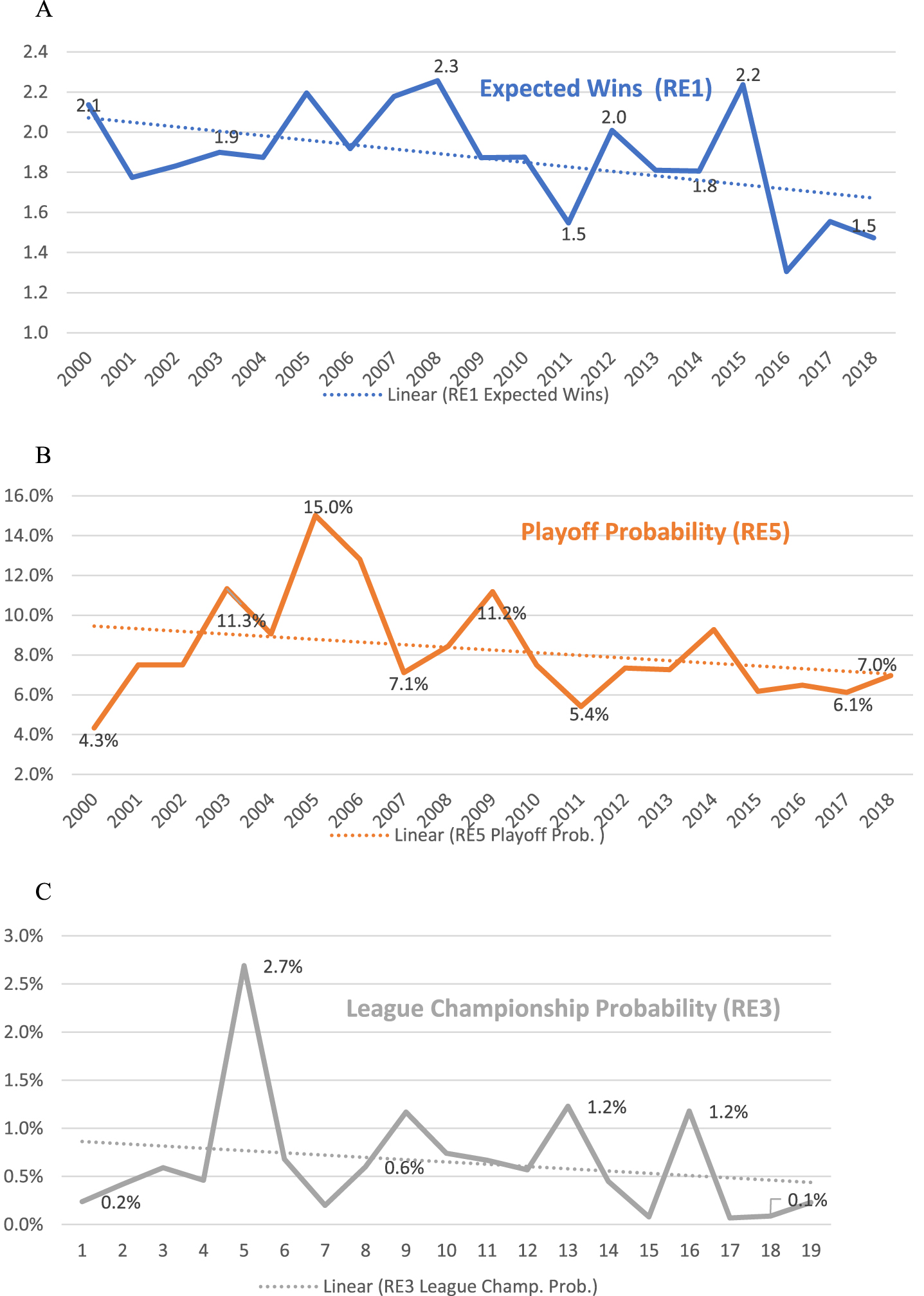
This reduction in schedule inequity over time is illustrated in Figs. 2A, 2B, and 2C. Figure 2A plots the trend line for the range of effects on the expected number of wins for each team (RE1), Fig. 2B plots the probability of making the playoffs (RE5), and Figure 2C plots the probability of being the NBA champion (RE3). The figures show a definite downward trend in all three measures, especially in RE3 (Fig. 2C), and significant variability in RE5 (Fig. 2B). As we have noted, independent of SFVs, teams’ chances of making the playoffs are affected by how many teams are in contention to make the playoffs, and teams’ chances of winning the NBA championship are affected by the existence (or not) of one or two dominant teams, which can change a great deal from year to year. In addition, RE3 (Fig. 2C) is significantly lower than RE5 (Fig. 2B), as noted in our earlier discussion in Table 4.
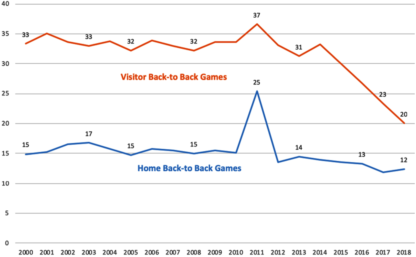
A major contributor to this clear downward trend in schedule inequity was the NBA reducing the number of back-to-back games—the single largest contributor to schedule inequity—played by teams. Fig. 3 shows the percentage of games where the visiting and home teams played back-to-back, separately. We have included the lockout-shortened 2011–12 season to demonstrate the dramatic effect of a compressed time frame. Ignoring that data point, we see that the percentage of home and visitor back-to-back games steadily decreased during the time frame, and the percentage of visitor back-to-back games dropped significantly in the last four seasons. The slope of the regression trend line, excluding the 2011 season, is –.195 % per year for home back-to-back games (p < .0001) and –.513 % per year for visitor back-to-back games (p-value.0005).
Fig. 3
Percentage of back-to-back games.
3.2Alternatives for minimizing schedule inequity
We believe that the ability to do retrospective analyses on an ongoing basis similar to what we just presented will be very useful. The approach would be very similar for prospectively evaluating any proposed schedule for an upcoming season with the exception that the team quality measures that combine with the SFV’s to determine the game win probabilities are not known prior to the season. We will discuss this point later in this section.
To incorporate the measures in prospective generation of schedules would be a complex undertaking and would require extensive data on factors such as arena availability. It would also need to incorporate potentially complex scheduling algorithms that fall in the realm of sports timetabling. This is well beyond the scope of this study, and we leave it for future research. We were, however, able to conduct some broad-brush experimentation that provides insights into how our measures might be best utilized in prospective schedule development that would properly consider schedule inequity.
Table 9
Schedule-adjustment impact on average schedule inequity measures
| Adjustment level | Expected wins (1) | Expected wins (Avg. var. effect) (2) | League champ. prob. (3) | Conf. champ. prob. (4) | Playoff prob. (5) | League rank (6) | Conference rank (7) | |
| Wins | 25% | 14.6 | 11.5 | 30.3 | 26.2 | 11.8 | 15.3 | 15.6 |
| 50% | 34.5 | 11.4 | 45.7 | 45.5 | 23.3 | 36.1 | 36.8 | |
| 75% | 67.1 | –20.0 | 65.6 | 64.1 | 41.3 | 62.1 | 60.7 | |
| Wins | 25% | 8.1 | 15.7 | 11.4 | 12.1 | 11.3 | 13.0 | 13.4 |
| Average | 50% | 16.3 | 38.1 | 11.4 | 12.1 | 25.3 | 27.6 | 26.3 |
| Effect | 75% | 25.0 | 68.9 | 20.0 | 25.4 | 39.9 | 44.8 | 42.2 |
| Random var. | 25% | 3.3 | –7.5 | 22.9 | 13.6 | –8.1 | –3.2 | 0.2 |
| Frequency | 50% | 20.6 | –8.7 | 25.7 | 15.2 | –1.4 | 2.2 | 4.4 |
| Reduction | 75% | 44.9 | 16.7 | 48.6 | 45.5 | 18.8 | 28.9 | 29.8 |
| Balanced var. | 25% | 23.6 | 16.5 | 20.0 | 22.4 | 17.2 | 19.7 | 21.3 |
| Frequency | 50% | 38.2 | 20.2 | 36.4 | 31.7 | 21.2 | 27.9 | 27.6 |
| Reduction | 75% | 49.4 | 25.5 | 50.0 | 48.5 | 27.6 | 33.5 | 35.0 |
Table 10
Schedule-adjustment impact on range inequity measures
| Adjustment level | Expected wins (1) | Expected wins (Avg. var. effect) (2) | League champ. prob. (3) | Conf. champ. prob. (4) | Playoff prob. (5) | League rank (6) | Conference rank (7) | |
| Wins | 25% | 29.8 | 5.4 | 36.6 | 33.7 | 16.5 | 19.6 | 17.8 |
| 50% | 51.4 | –4.6 | 52.0 | 51.7 | 31.5 | 41.4 | 40.7 | |
| 75% | 76.0 | –55.7 | 66.4 | 65.2 | 42.8 | 62.7 | 58.6 | |
| Wins | 25% | 9.5 | 30.5 | 9.3 | 12.9 | 15.8 | 21.6 | 18 |
| Average | 50% | 14.3 | 53.3 | 6.5 | 8.2 | 32.0 | 35.2 | 30.4 |
| Effect | 75% | 20.6 | 75.5 | 10.9 | 17.4 | 45.0 | 50.1 | 47.3 |
| Random var. | 25% | 12.4 | –8.6 | 32.1 | 20.6 | –11.7 | –4.3 | –0.9 |
| Frequency | 50% | 19.9 | –7.5 | 33.9 | 25.5 | –11.7 | 0.1 | 3.4 |
| Reduction | 75% | 43.5 | 15.6 | 56.5 | 55.5 | 11.1 | 26.2 | 23.2 |
| Balanced var. | 25% | 24.5 | 13.5 | 18.0 | 20.1 | 16.3 | 18.7 | 19.6 |
| Frequency | 50% | 41.3 | 19.0 | 34.0 | 33.7 | 27.3 | 29.9 | 30.0 |
| Reduction | 75% | 46.6 | 21.5 | 58.3 | 58.0 | 30.1 | 32.3 | 31.6 |
We adjusted the actual league schedules each year using four different approaches. The first two were based on the idea that schedule makers could look for teams with expected win effects that were most advantaged and disadvantaged by SFVs and focus adjustments on those teams. For these approaches, we switched all SFVs involved in two games in a pairwise fashion so that neither the frequency of SFV occurrences in total nor the frequency with which each SFV occurred in combination with other SFVs changed. The most advantaged or disadvantaged team was always involved in the switch. Moreover, the specific game to switch and the game to switch it with were chosen for maximal impact on the gap between the most advantaged and disadvantaged teams. In both the first and second approaches, these pairwise switches were based on the expected win effect. In the second approach, the average variable effects independent of team quality were used. In both cases, we continued the switches until the gap between the most advantaged and most disadvantaged teams (RE1 and RE2, respectively) was reduced by 25%, 50%, and 75%.
Our third and fourth schedule-adjustment approaches involved reducing the occurrence of SFVs. The third approach was to reduce occurrences across games randomly. To do so, we assigned to each SFV occurrence a probability of being eliminated from each game. The fourth approach was to balance the reduction in the occurrence of SFVs across teams. We examined 25%, 50%, and 75% random reductions and the same for balanced reductions.
Tables 9 and 10 present the results of our schedule-adjustment experiments. The adjustment strategies are listed on the side in the order described above. The schedule inequity measures are listed at the top. Each cell contains, in order, the percentage reduction in the inequity measure realized (a negative means it increased) when the schedule-adjustment approach was implemented at the 25%, 50%, and 75% levels. Table 9 shows the effect on the average schedule inequity measures and Table 10 on the range inequity measures. All simulation results are based on the same simulation strategy as the original measures (1000 replications of each season with 100 playoff replications for each season replication).
Comparing the first two approaches, we see that correcting imbalances is more effective when based on the SFV effects on the expected win of individual games (Column 1) rather than on the expected wins using the average effect (Column 2) of the SFVs. However, the former approach requires knowing the relative team strengths (the control variables in the statistical model) ex-ante. Earlier in this section, we mentioned this same issue with prospectively evaluating any potential schedule. One could make assumptions about team quality (such as they would be the same as the previous season). Individual teams might be interested in evaluating their schedules to try to find ways to improve them by adjusting factors they influence such as arena availability using this approach, but this would likely be problematic for league-wide efforts. As described earlier, teams were affected unevenly based on their quality, and schedule adjustments to punish (or help) them could be considered unfair if they were based on team quality rather than exclusively on the schedule they face. The second (expected win using average effect) approach does not require that we know the relative team strengths and involves adjustments based strictly on the SFVs. This approach is quite effective in reducing inequity concerning playoff probabilities. The reductions achieved were essentially identical to those achieved using the first approach for this measure. This is important as we believe that playoff probability is likely the most important measure of schedule inequity to try to improve.
We also note that the first approach often increases schedule inequity with respect to the average win effect, whereas the second approach decreases schedule inequity using the win measure. Overall, we conclude that utilizing the average effect of the SFVs (the second approach) is preferable both for incorporating into schedule generation approaches and prospectively evaluating any potential schedule. It does not require the knowledge of the relative team strengths, uniformly reduces schedule inequity, performs almost identically with the first approach on the playoff probability measure (the most critical measure), and has the advantage of being philosophically fairer than the first approach.
When comparing the third and fourth approaches (which involve reducing the occurrences), we note that random reduction often increases schedule inequity, and balanced reduction substantially outperforms random reduction at the 25% level; the approaches converge as further reductions are made—the two are identical at a 100% reduction. Note that deep reductions in the frequencies across the board (such as at the 50% and 75% levels) would likely require a significant change in the total number of games, the length of the season, or both. It seems more likely that the reductions would be limited to levels (such as 25%) where it would be important to try to reduce the occurrences in a balanced fashion.
3.3Future research
The most obvious extension of this approach is to apply it to the National Hockey League (NHL), which has a schedule similar to that of the NBA. The approach would require minor modifications due to the NHL’s point system rather than wins and losses. We treated only schedule variables in our analysis and limited the role of each team’s opponents to that of the control variables. For sports with unbalanced schedules (such as MLB and NFL), it might be interesting to assess scheduling inequity in terms of the teams played.
A particularly interesting area for future investigation would be to examine whether an association exists between the frequency of injuries and travel schedules or other schedule factors. Baker (2020) noted that the “bubble” environment used by the NBA in late 2020 appears to have reduced injuries and improved the quality of play. Since the NBA is widely regarded as a “star” league, the loss of key players in the league might affect attendance, viewership, or league ranking. Although this may not seem directly related to schedule inequity, we note that teams that face schedules associated with injury risks would indeed be placed at a competitive disadvantage if injuries to key players occurred.
4Conclusions
Assessing schedule inequity requires (1) a comprehensive model of the relative effects of schedule factors on game outcomes, (2) an approach for assessing these effects on each team across an entire season, and (3) a characterization of the imbalances (inequities) of these effects across the entire league. Our study contributes to the schedule inequity literature by providing an approach for accomplishing these three tasks. The reference 22 schedule and the importance of treating not only the schedule factors faced by each team but also by its opponents are vital contributions that enable these tasks to be effectively accomplished.
When we applied our approach to the NBA, we found that scheduling inequity has historically been significant but not severe. In the 19 years studied, we found that the most significant inequity was the effect of the schedule variables on the probability of making the playoffs, with an average range of effects of .0825 between the most advantaged and most disadvantaged teams. The economic consequences of making the playoffs are substantial, so this result has practical and theoretical importance.
In addition, we found that the NBA reduced scheduling inequity across the time frame. In particular, the NBA significantly reduced the number of back-to-back games (and their effect on inequity), especially in the last four seasons. This has been crucial for achieving schedule inequity reduction, as back-to-back games are the single most significant scheduling factor, accounting for 38% of our impact and imbalance measures.
We identified many other variables that have an impact on schedule inequity. Although adjusting schedules considering all the variables involved is a huge undertaking that requires all the data the NBA utilizes (such as arena availability), we examined alternative adjustments that provided some important insights that can help inform future research on sports timetabling. We showed that an adjustment using only average variable effects and the frequency of imbalances among teams is philosophically fair and reasonably effective. Efforts to reduce schedule inequity are most effective when considering both imbalances and raw frequencies but addressing imbalances is the most important.
Acknowledgments
We would like to thank James Lambrinos and several anonymous referees for invaluable comments that greatly improved the exposition of the paper.
Declaration of interest
The authors report that there are no competing interests to declare.
References
1 | Ashman, T. , Bowman, R.A. , & Lambrinos, J. , (2010) . The role of fatigue in NBA wagering markets: The surprising “home disadvantage situation”, Journal of Sports Economics, 11: (6): 602–613. |
2 | Baker, K. 2020, September 23. Less travel is causing the NBA to see better basketball, Axios. Available from:https://www.axios.com/nba-bubble-play-quality-travel-a1a48cc5-8760-48c5-8417-1d846aabf0fb.html. Accessed9/23/2021 |
3 | Bean, J.C. , & Birge, J.R. , (1980) . Reducing travelling costs and player fatigue in the National Basketball Association, INFORMS Journal on Applied Analytics, 10: , 98–102. |
4 | Duran, G. , Duran, S. , Marenco, J. , Mascialino, F. , & Rey, P.A. , (2019) . Scheduling Argentina’s professional basketball leagues: A variation on the Travelling Tournament Problem, European Journal of Operational Research, 275: ((3)), 1126–1138. |
5 | Entine, O.A. , & Small, D.A. , (2008) . The role of rest in the NBA home-court advantage, Journal of Quantitative Analysis in Sports, 4: (2), 1–9. |
6 | Goossens, D. , Yi, X. , & Bulck, D. (2020) . Fairness trade-offs in sports timetabling, In C. Ley & Dominicy, Y. (eds.) Science meets sports: When statistics are more than numbers. Newcastle upon Tyne, England: Cambridge Scholars Publisher, pp. 213–244. Available from: http://ebookcentral.proquest.com/lib/uleth/detail.action?docID=6370348 |
7 | Gough, C. , 2020. Total Revenue of the National Basketball Association 2001–2019, Statista.com. https://www.statista.com/statistics/193467/total-league-revenue-of-the-nba-since-2005/ |
8 | Hanley, J.A. , & McNeil, B.J. , (1982) . The meaning and use of the areaunder a receiver operating characteristic (ROC) curve, Radiology, Radiology 143: , 29–36. |
9 | Henz, M. , (2001) . Scheduling a major college basketballconference—Revisited, Operations Research, 49: (1), 163–168. |
10 | Huyghe, T. , Scanlan, A. , Dalbo, V. , & Calleja-Gonzalez, J. , (2018) . The negative influence of air travel on health and performance in the National Basketball Association: A narrative review, Sports, 6: (3), 89. Available from: https://doi.org/10.3390/sports6030089 |
11 | Karwan, M. , Kurt, M. , Pandey, N.K. , & Cunningham, K. , 2015. Alleviating competitive imbalance in NFL schedules: An integer-programming approach. In 9th Annual MIT Sloan Sports Analytics Conference, Boston, MA. |
12 | Kelly, Y.J. , (2010) . The myth of scheduling bias with back-to-back games in the NBA, Journal of Sports Economics, 11: ((1)), 100–105. |
13 | Murray, T.J. , (2018) . Examining the relationship between scheduling and the outcomes of regular season games in the National Football League, Journal of Sports Economics, 19: (5), 696–724. |
14 | Roy, J. , & Forest, G. , (2018) . Greater circadian disadvantage during evening games for the National Basketball Association (NBA), National Hockey League (NHL) and National Football League (NFL) teams travelling westward, Journal of Sleep Research, 27: (1), 86–89. |
15 | Schaefer, R. , 2020. Report: NBA could lose “nearly $ million” in ticket revenue without games, nbcsports.com. Available from: https://www.nbcsports.com/chicago/bulls/report-nba-could-lose-nearly-500-million-ticket-revenue-without-games. [12 March 2020]. |
16 | Van Voorhis, T. , (2002) . Highly constrained college basketball scheduling, The Journal of the Operational Research Society, 53: ((6)), 603–609. |
17 | Van Voorhis, T. , (2005) . College basketball scheduling with travel swings, Computers & Industrial Engineering, 48: (2), 163–172. |
18 | Wright, M.B. , (2006) . Scheduling fixtures for Basketball New Zealand, Computers & Operations Research, 33: (7), 1875–1893. Available from: https://doi.org/10.1016/j.cor.2004.09.024 |
19 | Yang, F.C. , 2017. NBA sports game scheduling problem and GA-based Solver, In 2017 International Conference on Industrial Engineering, Management Science and Application (ICIMSA). IEEE, pp. 1–5. Available from: https://doi.org/10.1109/ICIMSA.2017.7985598 |
Notes
1 Our complete model of schedule factors includes 20 variables (SFVs), which are listed and described in Table 1 in Section 2. The remaining variables had limited differential effect on these two teams (Table 3); comparing any two teams in any season in a similar manner involved different combinations of the SFVs having the largest effects.
2 Note that this was only counted when the game being played was not back-to-back, so it is separate from the effect in the previous item.
3 A similar pattern has been observed in the scheduling of bye weeks for NFL games (Karwan et al., 2015; Murray, 2018).
4 Bean and Birge (1980) reported that travel distances affect game outcomes. Roy and Forest (2018) stated that the number of time zones crossed and playing in the afternoon or evening affect game outcomes.
5 Duran et al. (2019) developed a software for the Argentine basketball league that solved the timetabling to minimize travel length in the first round; then allowed the user to enter preferences for minimizing back-to-back games and for fairness in the distribution of scheduling factors in the second round. Other examples are Wright (2006) for New Zealand and Henz (2001) and Van Voorhis (2002, 2005) for NCAA conferences.
6 The reference schedule can be thought of as a sparse 2-day rest schedule.
7 We could have just used dummy variables for the two teams that played and for the home court advantage. However, having dummy variables for the home team and away team allowed different effects for each team at home and away, improving the fit. Although the coefficients of these control variables are quite interesting, they are not instructive for schedule inequity and are far too numerous to present; therefore, we have not included them here. We also note that the overall model fit is statistically significant with a p-value below.0001 just using the control variables, so the decisions on which schedule variables to include in the model were based on their marginal effect on the fit as described above.
8 The area under the receiver operating characteristic (ROC) curve is a common measure of ability to discriminate between two outcomes, win or lose in our case (see, for example, Hanley & McNeil, 1982).
9 We did a sensitivity analysis, first deleting variables SFV17– SFV20 and then the first 12 variables with p-values >.05. We reported these results later, but our conclusions were not sensitive to whether these variables were included.


