
How to schedule the Volleyball Nations League
Abstract
The Volleyball Nations League is the elite annual international competition within volleyball, with the sixteen best nations per gender contesting the trophy in a tournament that spans over 6 weeks. The first five weeks contain a single round robin tournament, where matches are played in different venues across the globe. As a consequence, each team follows an intensive travel plan, where it happens quite often that there is a large discrepancy between travel burdens of opposing teams. This is considered a disadvantage for the team that travelled more. We analyse this problem, and find that it is closely related to the well-known Social Golfer Problem: we name the resulting problem the Traveling Social Golfer Problem (TSGP). We propose a decomposition approach for the TSGP, leading to the so-called Venue Assignment Problem and the Nation Assignment Problem. We prove that a solution to the Venue Assignment problem determines the amount of unfairness, and we also prove that any solution of the Venue Assignment problem can be extended to a solution to the Nation Assignment problem satisfying the so-called home-venue property. Using integer programming methods, we find, for real-life instances, the fairest schedules with respect to the difference in travel distance.
Prologue
It is the beginning of June 2018 when the Italian men volleyball team go undefeated in the first round of the inaugural Volleyball Nations League. They played their three first-round matches in Kraljevo, Serbia, and for the next round of three matches they have to travel, via Belgrade, Rome, Buenos Aires, to reach the next venue in San Juan, Argentina, after more than 24 hours of traveling. Playing only a few days after this trip, their momentum seems lost and they lose two out of their three games, all played within a week, upon which they immediately need to fly to Japan for the third round.
Ultimately, the Italian team had to travel literally across the globe within a time span of four weeks, playing matches against the best volleyball teams in the world. Even though they started off with three victories, they ended eighth and did not qualify for the final stages. In comparison, the French team played all their matches within Europe and emerged as winner of the main event. Later that year however, during the World Championship, the Italian team outperformed the French team.
1Introduction
The above example is just one of many that highlights how travel times, and specifically disparity in travel times, influence results in the Volleyball Nations League (VNL). It is well established within the scientific literature that extensive travelling has a negative impact on sport performance. Although we do not intend to survey the literature on this subject, this finding is reported for various sports ranging from rugby (Lo et al. (2020)) to baseball (Song et al. (2017), and Winter et al. (2009)) and from basketball (Huyghe et al. (2018)) to triathletes (Stevens et al. (2018)); see also the references contained in these papers. We close this paragraph by two quotes: one from an interview with Anne Buijs, professional volleyball player(see Volkskrant (2021)): “It is quite an advantage to play all VNL matches at the same location. In the original schedule we would have travelled from Serbia to Canada to Korea, which makes the schedule very hard for us.”, and one from Samuels (2012) who concludes: “Jet lag and travel fatigue are considered by high-performance athletic support teams to be a substantial source of disturbance to athletes.” This phenomenon is illustrated in the prologue of this paper, and serves as its motivation.
The Volleyball Nations League is a tournament organized every year by the FIVB (Fédération Internationale de Volleyball), for both men and women (see https://www.volleyball.world/en/vnl/2021). This tournament was first organized in 2018 to replace the World League/World Grand Prix as annual volleyball tournament. There are 16 teams participating in the tournament which consists of multiple phases. In the first phase, lasting for five weeks, all 16 teams play a single round robin, i.e., each team meets each other team once. The best 6 teams then qualify for the second phase, where out of two groups of three, four teams emerge to play cross finals. Our interest is exclusively on the first phase.
In the first phase of the VNL tournament, teams play in rounds. In each round, each team is in a group consisting of 4 teams, and each team in a group plays a match against its three fellow group members. After 5 rounds, each of the 16 teams has played all the other teams exactly once, and a ranking is made based on the results in this single round robin tournament. All 6 matches in a single group are held at the same venue, however, every round has its 4 groups played out in different venues. As it is a disadvantage to have traveled more than your opponent going into a match, our main interest lies in minimizing a measure that captures the imbalance in travel times between opposing teams.
A priori, it is not clear how a round robin schedule that can be decomposed in groups is obtained. In fact, finding a schedule that fits this VNL-format is related to the so-called Social Golfer Problem (SGP). In this problem we are given gp golfers and w rounds (where g, p, w are positive integers), and the SGP-question is whether it is possible to let the gp golfers play in g groups of p golfers in each of the w rounds, in such a way that every pair of golfers plays in the same group in at most one round, see Triska & Musliu (2012), Liu et al. (2019), Dotú & van Hentenryck (2005). This question is far from innocent: only for restricted sets of values for g, p, w the answer to this question is known. For instance, when g = p = w - 1, solutions are known to exist when g is a prime power - and no other solution to these type of instances has been found, nor has it been proven that these are the only instances for which a solution can exist (Harvey & Winterer (2005)).
Of course, in the context of the Volleyball Nations League, each golfer corresponds to a team (and groups remain groups and rounds remain rounds). Since the Volleyball Nations League has g = p = 4 and w = 5, it follows that the answer to the SGP-question is affirmative, and hence a schedule for the VNL that consists of 5 rounds, each round consisting of 4 groups, is known to exist. In this paper, we introduce the Traveling Social Golfer Problem (TSGP), as a generalization of the SGP; the TSGP allows us to take fairness, as measured by the difference in travel times between opposing teams, into account. Recent other variations of the SGP are discussed in Miller et al. (2021) and Lester (2021).
A well-known problem related to the TSGP that also focusses on distances is the Travelling Tournament Problem (TTP), see Easton et al. (2003) for a precise description. In contrast to our problem, in the TTP pairs of teams meet in the venue of one of the two opposing teams. Moreover, the objective in the TTP is to minimize total travel distance; difference in travel time between opposing teams is not considered in the TTP. We refer to Goerigk & Westphal (2016) and Durán et al. (2019) for an overview concerning the TTP.
A number of studies has been devoted to the scheduling of national volleyball leagues where mainly for cost reasons, the objective is to minimize total travel time. We mention Bonomo et al. (2012) who model the Argentine national volleyball league as an instance of the Traveling Tournament Problem, and Cocchi et al. (2018) who investigate the Italian volleyball league. Further, Raknes & Pettersen (2018) study the Norwegian Volleyball League; one of their models, motivated by a cost-objective, is devoted to minimizing total travel distance in that league. These leagues are organized in the format of a Double Round Robin, and as such differ from the VNL.
2The Traveling Social Golfer Problem (TSGP)
2.1Definition of the TSGP
As described in Section 1, the Social Golfer Problem is a well known combinatorial question, where the task is to schedule golfers in groups of size p over multiple rounds, such that no golfer plays with another golfer in the same group twice. In the Traveling Social Golfer Problem (TSGP), all groups have to play at (different) venues, where the objective is to create a schedule that minimizes the unfairness arising from golfers having different travel times between the venues.
In order to give a precise formulation of the TSGP, we use the following notation to describe the input:
• N: the number of teams,
• k: a group size,
• V: the set of venues,
• d (v, w): a distance between each pair of venues v, w ∈ V, and
• cv: a multiplicity for each v ∈ V.
Furthermore, we use the following notation to describe a solution:
• R: a set of rounds,
•
• vr (t): the venue of the group in which team t ∈ {1, …, N} plays in round r ∈ R.
Finally, we measure the value of a schedule S by its unfairness u (S) as follows:
(1)
Let us elaborate on this expression. For every group
Example 2.1. A tournament with N = 4, teams 1, 2, 3, 4, is organized over three rounds, and groups of size k = 2. There are four venues, V = {A, B, C, D}, with multiplicities cA = cD = 2 and cB = cC = 1. Distances between venues are d (A, B) = d (A, C) = d (B, D) = d (C, D) =1 and d (A, D) = d (B, C) =2.
Consider the schedule S depicted in Table 1.
Table 1
A schedule S for the instance in Example 2.1
| group | venue | group | venue | |
| round 1 |
| A |
| D |
| round 2 |
| A |
| B |
| round 3 |
| D |
| C |
Thus, according to (1), the unfairness of this schedule S equals:
We state the following optimization problem that we call the (N, k)-Traveling Social Golfer Problem, or (N, k)-TSGP for short.
Problem 2.1. (N, k)-TSGP
Input. A number of teams
Output. A schedule S consisting of |R| rounds minimizing u (S) such that:
• there is an equi-partitioning of N teams in groups
• an allocation of groups to venues that results in venues vr (t) (r ∈ R, t = 1, …, N) such that venue v ∈ V acts cv times as a host for a group.
It is clear that, depending on the input, a feasible schedule to (N, k)-TSGP need not exist; in fact, it is not difficult to find instances where there is no schedule S that satisfies all the constraints. Indeed, as the schedule asks for a partitioning of the N teams in groups of size k in each round, we immediately see that N should be a multiple of k, or N ≡ k0. In addition, as the schedule should correspond to a single round robin tournament, and as all teams play k - 1 matches per round, we conclude that N - 1 should be a multiple of k - 1, or (N - 1) ≡ k-10. Thus, a solution of the (N, k)-TSGP can only exist if there is an integral ρ such that N = k · ((k - 1) ρ + 1).
The above are necessary conditions that need to be satisfied. In fact, the (N, k)-TSGP can only have a solution that satisfies the single round robin format, if the corresponding instance of the SGP is solvable. In general, solutions of the SGP are known to exist when N = k2 and k is a prime power. Thus, for the Volleyball Nations League, the underlying N = 16, k = 4-SGP problem will be solvable. In the remainder of the paper, we assume that N = k2 and |R| = k + 1; this ensures that the above necessary conditions are fulfilled (and observe that the VNL case arises when k = 4).
2.2Decomposing the TSGP into Venue Assignment and Nation Assignment
The problem of solving an instance of (N = k2, k) - TSGP can be decomposed into two phases:
• Venue Assignment. In the first phase, we specify, for each round r ∈ R, which venues act as a host. Let Ur ⊂ V, with |Ur| = k, r = 1, …, k + 1 be the set of venues that act as hosts in round r.
• Nation Assignment. In the second phase, we decide upon the composition of the groups, i.e., we choose the sets
By going through these two phases, we find a schedule S. It is crucial to observe that the unfairness of S, i.e., u (S), follows directly from the venue assignment when N = k2. We record this observation formally.
Theorem 2.1. For each schedule S of a given instance of (N = k2, k) - TSGP, u (S) is determined only by the Venue Assignment, for each integer k ≥ 2.
Proof. We claim that for each schedule S:
The latter equality follows from the fact that, independent of the composition of the groups, the k teams that play in a group in some round, will not meet again in a next round, and hence these k teams will travel to each of the k distinct venues in the next round. □
Theorem 2.1 allows us to compute the unfairness of a schedule S, u (S), without specifying the schedule S. As a consequence, it becomes much easier in practice to find schedules for which u (S) is minimum. Or, rephrasing Theorem 2.1, finding a Venue Assignment suffices to know the unfairness of any schedule compatible with the Venue Assignment. In fact, a similar statement can be made with respect to the total travel time (see Section 5).
3The complexity of Venue Assignment
In this section, we formally establish the complexity of Venue Assignment. Given that feasible schedules to the (N = k2, k)-TSGP exist, Theorem 2.1 implies that our task of finding an optimal solution to (N, k)-TSGP is reduced to finding an optimal venue assignment. Clearly, this is related to the differences in traveled distance between two opposing teams, which in turn follows from the venues that are selected in each round.
In an extreme case, if only a single venue v is given (with multiplicity cv = k (k + 1)), then all matches in all groups in all rounds are played in the same venue, and there is no travel distance. However, in general, the set of venues V and their pairwise distances, are instrumental in finding good venue assignments. Of course, we assume that ∑v∈Vcv = k (k + 1). We now give a formal description.
Problem 3.1. Venue Assignment (VA)
Input. A value
Output. For r ∈ {1, …, k + 1}, subsets Ur ⊂ V with |Ur| = k, such that ∀v ∈ V, cv = | {r : v ∈ Ur} | that minimizes:
(2)
To establish the hardness of Venue Assignment, we use the following decision problem.
Problem 3.2. Longest Hamiltonian Path on a Complete Graph (LHP)
Input. A complete graph G = (H, E), |H| = n with nonnegative, symmetric weights w (h1, h2) for each h1, h2 ∈ H, and an integer B.
Question. Does there exist a Hamiltonian Path (hi1, …, hin) in G such that
LHP is well-known to be NP-complete.
Theorem 3.1. Venue-Assignment is NP-Hard.
Proof. We prove this statement by a reduction from Longest Hamiltonian Path on a Complete Graph.
Given an instance of LHP, with vertex set H = {h1, …, hn} and weights
We choose k : = n - 1. Further, the set of venues V consists of V = V1 ∪ V2, where V1 : = H and |V2| : = n - 2. For each v ∈ V1, cv : =1 and for each v ∈ V2, cv : = n. Let
(3)
Notice that the resulting distances satisfy the triangle inequality when the instance of LHP does. Finally, we set K : = k2 · 2D - B, and ask whether there exists a venue assignment with unfairness at most K. We have now specified an instance of the decision version of VA.
Let us argue that if there exists a solution to VA with unfairness at most K, LHP is a yes-instance, and vice versa.
To find a solution to any instance of VA, we need to find Ur ⊂ V for each r ∈ {1, …, k + 1} such that ∀v ∈ V, cv = | {r : v ∈ Ur} |. As we know that for all v ∈ V2, cv = k + 1, we see that any feasible solution must have V2 ⊂ Ur for each round r. Moreover, as cv = 1 for v ∈ V1, we get that any feasible solution must schedule every venue v ∈ V1 exactly once. Thus, any feasible solution to VA consists of Ur = V2 ∪ vir with vir ∈ V1 and
(4)
Let us now suppose that the instance of LHP is a yes-instance, implying the existence of a Hamiltonian Path such that
(5)
(6)
(7)
(8)
Finally, suppose there exists a schedule S whose unfairness is bounded by K, we obtain:
(9)
(10)
Thus, solving this instance of the decision version of VA is equivalent to solving the corresponding instance of LHP, which implies that VA is NP-Hard. □
4The VNL in practice: about the home-venue-property
Motivated by the current practice in the VNL, we incorporate the following issue in our problem formulation: each venue has a team that considers this venue as its home-venue. Next, in any feasible schedule for the VNL it must be the case that when a venue is hosting a group, the group must contain the team for which this venue is the home-venue. And in case there are multiple venues that are the home-venue of the same team, it is a fact that those venues are never a host of a group in the same round. Thus, each venue is a home venue to a single team; however, a team can have multiple home venues. In the context of the VNL, this property specifies that each venue always hosts a group that contains the national team; this team can be regarded as the home playing team, or host nation. As an aside, it is interesting to note here that Alexandros et al. (2012) find the presence of (a significant) home advantage in volleyball matches played in Italian and Greek national leagues.
We will refer to solutions having the property that the venue hosting a group is the home-venue for some member of the group, as the home-venue property. A relevant question now becomes:
Do feasible schedules satisfying the home-venue property exist?
In fact, solving the Venue Assignment problem does not automatically lead to a schedule that satisfies the home-venue property. In other words, it is not true that, when given an assignment of venues to rounds, a schedule is guaranteed to exist such that every venue is a home venue. Then, in such a case, a venue hosts a group of teams, none of which plays home. Example 4.1 shows how a feasible solution of the Venue-Assignment problem cannot be extended to a solution having the home-venue property.
Example 4.1. Let N = 4 be the number of teams with group size k = 2, and let V be the set of home venues. All countries t have a venue vt ∈ V, where for countries t = 1, 2, their venue has a multiplicity of 2 and the other venues have a multiplicity of 1, i.e., cv1 = cv2 = 2 and cv3 = cv4 = 1. Solving the corresponding instance of Venue-Assignment can result in a solution as is given in Table 2.
Table 2
A venue-assignment that does not satisfy the home-venue property
| Group | Round 1 | Round 2 | Round 3 |
| 1 | v1 | v1 | v3 |
| 2 | v2 | v2 | v4 |
The venue assignment in Table 2 clearly satisfies the given multiplicities. However, it is impossible to schedule match (t1, t2) in any round when restricting teams to play at their home venue whenever it is scheduled in a round. Moreover, venue assignments satisfying the given multiplicities yielding a feasible schedule do exist for the given example.
Thus, we see that solving the Venue-Assignment alone is not necessarily the same as solving the VNL-problem in practice.
However, and perhaps surprisingly, the following theorem shows that for the particular dimensions of the VNL (N = 16, k = 4), a Venue-Assignment can always be extended to a solution for the Volleyball Nations League.
Theorem 4.1. Let N = 16 be the number of teams and k = 4 the group size. Let V be the set of venues, with corresponding multiplicities cv (v ∈ V) such that each team has at least one home venue, and all venues need to be scheduled at least once (never with two venues of the same team hosting simultaneously), i.e., cv ≥ 1 for each v ∈ V, and ∑v∈Vcv = 20. Then any solution of the corresponding Venue-Assignment instance, can be extended to a feasible solution of the VNL-instance satisfying the home-venue property.
Proof. We organize the proof as follows. First, we specify the groups (called our ‘blueprint’). Second, we provide a partial designation of home venues. Then we consider the possibilities that exist for the vector cv, and for each of these possibilities, we consider the set of distributions over the rounds. Finally, we outline how, for each of these distributions, we can arrive at a solution that satisfies the home-venue property.
Consider Table 3, where column “Ri” stands for Round i, i = 1, …, 5, and where each number from {1, …, 16} stands for a team. We refer to this composition of groups as a ‘blueprint’, and we will argue that, for any possible set of multiplicities, and for any distribution of these multiplicities over the rounds, this blueprint can be turned into a venue assignment satisfying the home-venue property, and hence into a nation assignment.
Table 3
Blueprint that specifies the composition of the groups
| R1 | R2 | R3 | R4 | R5 |
| 1, 5, 9, 13 | 1, 6, 11, 16 | 1, 4, 10, 15 | 1, 3, 12, 14 | 1, 2, 7, 8 |
| 2, 6, 10, 14 | 2, 5, 12, 15 | 2, 3, 13, 16 | 2, 4, 9, 11 | 3, 4, 5, 6 |
| 3, 7, 11, 15 | 3, 8, 9, 10 | 6, 7, 9, 12 | 5, 7, 10, 16 | 10, 11, 12, 13 |
| 4, 8, 12, 16 | 4, 7, 13, 14 | 5, 8, 11, 14 | 6, 8, 13, 15 | 9, 14, 15, 16 |
Of course, Table 3 does not constitute a feasible solution, as it has not been specified for each group which team plays at its home-venue. This clearly depends on the multiplicities; in Table 4, we provide a partial specification of the teams that play at their home-venue.
Table 4
Partial and provisional designation of teams that act as host
| R1 | R2 | R3 | R4 | R5 |
| 1 | · | · | · | · |
| 2 | 12 | 16 | 11 | 6 |
| 3 | 10 | 9 | 5 | 13 |
| 4 | 7 | 8 | 15 | 14 |
In fact, Table 4 provides an initial assignment such that each team is the host in exactly 1 group, i.e., each of the numbers 1, …, 16 occurs once.
We will now identify all possibilities for cv, the vector of multiplicities. Without loss of generality, we can assume that the entries in this vector are non-increasing. As stipulated in Theorem 4.1, we have cv ≥ 1 for each v ∈ V, and ∑v∈Vcv = 20, which implies that there exist 5 distinct possibilities for the first four entries of cv, namely:
(11)
It is important to realize that, for each of these possibilities, the distribution of the multiplicities over the rounds may differ, and that each of these distributions should be considered separately. As an example, consider the case where (c1, c2, c3, c4) = (3, 3, 1, 1). One possible solution of the Venue Assignment problem is that there are three rounds where the venues of both team 1 and team 2 are host. Another possible solution of the Venue Assignment problem is that in rounds 1, 2, 3, the venue of team 1 is host, whereas in rounds 3, 4, 5 the venue of team 2 is host. We refer to each such solution as a distribution. We call two distributions distinct when no permutation of the rounds maps one distribution to the other.
Given a particular choice for (c1, c2, c3, c4), it is not immediately clear how many pairwise distinct distributions exist. Let D (c1, c2, c3, c4) denote the set of pairwise distinct distributions compatible with (c1, c2, c3, c4). By a case analysis, we claim that |D (5, 1, 1, 1) |=1, |D (4, 2, 1, 1) |=2, |D (3, 3, 1, 1) |=3, |D (3, 2, 2, 1) |=11, and |D (2, 2, 2, 2) |=17. In fact, Table 5 displays the sets D (c1, c2, c3, c4).
Table 5
Extending the blueprint to a feasible schedule satisfying the home-venue property
| (c1, c2, c3, c4) | Multiplicity distribution | Teams to label | Altered Venues |
| over rounds (R1, …, R5), | |||
| i.e., D (c1, c2, c3, c4) | |||
| (5, 1, 1, 1) | (A, A, A, A, A) | A : 1 | |
| (4, 2, 1, 1) | (AB, A, A, A, B) | A : 1, B : 2 | |
| (AB, AB, A, A, -) | A : 1, B : 4 | R5 : 7 | |
| (3, 3, 1, 1) | (AB, A, A, B, B) | A : 1, B : 2 | R1 : 11, R4 : 3 |
| (AB, AB, A, B, -) | A : 1, B : 2 | R3 : 11, R4 : 12, R5 : 8 | |
| (AB, AB, AB, - , -) | A : 1, B : 2 | R1 : 16, R2 : 4, R4 : 12, R5 : 7 | |
| (3, 2, 2, 1) | (ABC, ABC, A, - , -) | A : 1, B : 2, C : 4 | R4 : 12, R5 : 7 |
| (ABC, AB, AC, - , -) | A : 1, B : 7, C : 8/ | R1 : 6, R4 : 3, R5 : 2, 4 | |
| (ABC, AB, A, C, -) | A : 1, B : 4, C : 3 | R5 : 7 | |
| (AB, AB, AC, C, -) | A : 1, B : 2, C : 12 | R2 : 14, R5 : 7, 9 | |
| (ABC, A, A, BC, -) | A : 1, B : 14, C : 11 | R4 : 6, R5 : 2, 3, 15 | |
| (ABC, A, A, B, C) | A : 1, B : 3, C : 2 | ||
| (AB, AC, A, BC, -) | A : 1, B : 2, C : 12 | R3 : 11, R5 : 8 | |
| (AB, AC, A, B, C) | A : 1, B : 3, C : 7 | ||
| (AB, AB, A, C, C) | A : 1, B : 4, C : 14 | R5 : 7 | |
| (AB, A, A, BC, C) | A : 1, B : 4, C : 14 | R3 : 11, R5 : 8 | |
| (A, A, A, BC, BC) | A : 1, B : 7, C : 14 | R2 : 5, 13, R5 : 12 | |
| (2, 2, 2, 2) | (ABCD, ABCD, - , - , -) | A : 1, B : 2, C : 3, D : 4 | R3 : 10, R4 : 12, R5 : 7 |
| (ABCD, ABC, D, - , -) | A : 1, B : 2, C : 3, D : 4 | R3 : 5, R4 : 10, 12, R5 : 8 | |
| (ABC, ABC, D, D, -) | A : 1, B : 2, C : 4, D : 15 | R4 : 12, R5 : 7 | |
| (ABCD, AB, CD, - , -) | A : 1, B : 2, C : 3, D : 4 | R3 : 5, R4 : 16, 12, R5 : 8 | |
| (ABCD, AB, C, D, -) | A : 1, B : 2, C : 4, D : 3 | R2 : 13, R5 : 7, 12 | |
| (ABC, ABD, CD, - , -) | A : 1, B : 2, C : 4, D : 8 | R2 : 13, R4 : 12, R5 : 7, 10 | |
| (ABC, ABD, C, D, -) | A : 1, B : 10, C : 4, D : 5 | R4 : 12, R5 : 2 | |
| (ABC, AB, CD, D, -) | A : 1, B : 2, C : 4, D : 11 | R4 : 12, R5 : 8 | |
| (ABC, AB, C, D, D) | A : 1, B : 3, C : 8, D : 14 | R2 : 4, R3 : 10, R5 : 7 | |
| (AB, AB, CD, CD, -) | A : 1, B : 4, C : 15, D : 16 | R2 : 5, R4 : 12, R5 : 7 | |
| (AB, AB, CD, C, D) | A : 1, B : 2, C : 15, D : 8 | R4 : 12 | |
| (ABCD, A, B, C, D) | A : 1, B : 4, C : 3, D : 2 | ||
| (ABC, AD, BD, C, -) | A : 1, B : 4, C : 3, D : 8 | R1 : 10, R5 : 2 | |
| (ABC, AD, B, C, D) | A : 1, B : 4, C : 3, D : 7 | ||
| (AB, AC, BD, CD, -) | A : 1, B : 4, C : 12, D : 11 | R5 : 8 | |
| (AB, AC, BC, D, D) | A : 1, B : 16, C : 4, D : 14 | R5 : 7 | |
| (AB, AC, BD, C, D) | A : 1, B : 4, C : 12, D : 8 |
We now describe how Table 5 can be read such that it provides a feasible solution satisfying the home-venue property for each distribution. To do so, we use the labels A, B, C, D for those teams whose home venues have a multiplicity higher than 1.
Each entry of Table 5 should be interpreted in the following way:
• Use the group composition from the blueprint in Table 3 and the partial venue assignment from Table 4 as a start. Notice that the latter may be altered; the former will not change.
• The second column in Table 5 gives the set D (c1, c2, c3, c4). Each of these entries indicates which labeled teams are hosts in round R1 to R5.
• The third column assigns a specific team to each label. As a consequence, this may induce a change to the partial venue assignment specified in Table 4. Indeed, the labeled team hosts a group in the rounds where it is supposed to be host according to its distribution specified in the second column.
• By exercising the previous step, some teams might lose their current group to host. In the fourth column “Altered Venues” additional changes to the schedule are denoted, where for every round altered compared to Table 4, the new hosting teams are given.
In this way, Table 5 gives, for every possible venue assignment, a schedule that satisfies the home-venue property, thereby completing the proof. □
Thus, Table 5 can be read as an instruction of how to find a feasible schedule satisfying the home-venue property for any solution of the Venue Assignment problem.
As an example, consider the distribution (ABC, AB, AC, - , -) which is an element of D (3, 2, 2, 1). The corresponding entries in the third column of Table 5 imply that in R1, teams 1, 7 and 8 act as host. Next the fourth column corresponding to this distribution, contains “R1 : 6”, implying that team 6 also acts as host in R1. Continuing in this way, it follows that teams 1, 12, 10, and 7 act as hosts in R2, teams 1, 16, 9, and 8 act as hosts in R3, teams 3, 11, 5, and 15 act as hosts in R4, and teams 2, 4, 13, and 14 act as hosts in R5. It is interesting to observe that in each of the schedules needed in the proof of Theorem 4.1, the composition of the groups as specified in the blueprint from Table 3 is identical.
Lastly, we like to point out that a nation might have multiple venues where it can/must host. In the proof of the previous theorem, we assumed every nation to have one venue with a specific multiplicity. When there are multiple venues, when calculating the travel distance it matters which one is used to host a group. To address this, we solve the Venue Assignment on the complete set of all venues, with the restriction that venues from the same nation cannot host in the same round. For the Nation Assignment however, it does not matter which venues are used specifically - in this stage, we only assign nations to groups, in such a way that a host nation will be scheduled to play in its own venue(s). Hence, when solving the Nation Assignment using the blueprint, we may assume that every nation has exactly one venue.
5Solving real-life instances of the VNL
In Section 5.1, we give an integer programming formulation of the Venue-Assignment Problem. Section 5.2 presents the outcomes.
5.1An Integer Programming Formulation
Let xv,r be the binary variables that indicate whether venue v ∈ V hosts a group in round r ∈ {1, …, 5} = R. Further, we need real variables sv,w,r (capturing distances between venues v and w acting as host in rounds r and r + 1), mv,r (capturing the largest distance traveled to venue v in round r), and Kv,r (capturing the difference in travel distance to venue v in round r). Let
(12)
(13)
(14)
(15)
(16)
(17)
(18)
(19)
(20)
First, observe that (12) captures the objective function, minimizing u = ∑v,rKv,r. Next, constraints (13) ensure that in every round, k venues are host; constraints (14) ensure that every venue hosts as often as required; constraints (15) ensure that two venues that should not host simultaneously, will not host simultaneously. Auxiliary variables sv,w,r are at least as large as dv,w, the distance traveled between venues w, v in rounds r - 1 and r if these venues host in the respective rounds, by constraints (16), but never larger than dv,w by constraints (17). The variables mv,r equal the maximum distances traveled to venue v in round r (can equal zero 0 if v does not host in round r), as defined by (18), and Kv,r resembles the difference in traveled distances towards v in round r compared to the maximum travel distance, where the terms -D · (1 - xw,r-1) in (19) nullify any influence caused by distances between a venue that does not host in round r - 1.
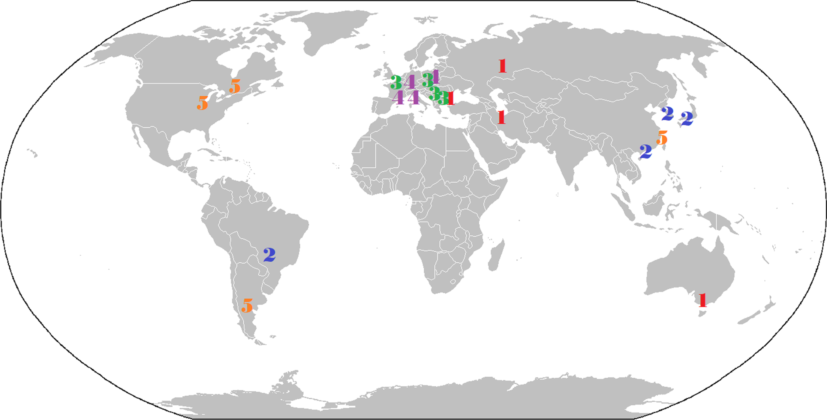
Fig. 1
Optimal venues per round, VNL Men 2018.
5.2Results
As instances of VNL satisfy the conditions of Theorem 4.1, we can proceed applying the integer programming formulation (12)–(20) for the Venue-Assignment to the known instances of the Volleyball Nations League, and compare our solution to that of the schedules used in practice. Formulation (12)-(20) is implemented in Python 3 using Gurobi 9.0. All computations have been done on a laptop with an Intel Core i7-7700HQ CPU 2.8-GHz processor and 32 GB RAM. The distances between venues are obtained via https://www.distancecalculator.net/, and are divided by 100 and rounded down. The four instances that we analyse are the Women’s and Men’s tournaments of 2018 and 2019. All values resulting from solving (12)-(20) are mentioned to be optimal by the solver and are found within approximately 2 hours of computation time.
In Table 6 we give the unfairness corresponding to the optimal venue assignment, u (Sopt), and we give the unfairness that corresponds to the venue assignments used in practice, u (Sreal). Also we give the total travel distance for the two corresponding solutions, d (Sopt) and d (Sreal), where the distance is given in units of 100 km. The final column gives the computation time in seconds.
Table 6
Unfairness of real life Sreal and optimal Sopt, and their total travel distance
| Instance | u (Sopt) | u (Sreal) | d (Sopt) | d (Sreal) | Computation time (s) |
| M2018 | 233 | 1366 | 4272 | 4806 | 5105s |
| W2018 | 381 | 1541 | 4956 | 4169 | 1036s |
| M2019 | 347 | 1239 | 5237 | 4657 | 7230s |
| W2019 | 491 | 1288 | 4214 | 3708 | 4650s |
As is imminent from Table 6, the fairness of the schedules used in the Volleyball Nations League can be much improved in comparison to the schedules that have been used. Moreover, these improvements in fairness do not come at the expense of the total travel distance; indeed, total travel distance is similar for our schedules when compared to the real life schedules.
We now discuss our schedules in more detail. In Table 7, the optimal schedule for the 2018 Men’s tournament is shown, and the corresponding venue assignment is also visualized in Fig. 1 –the output for the other instances is given in Appendix A. For comparison, the schedule used in practice is shown in Table 8. In Tables 9–11 optimal venue assignments are shown for Men and Womens tournaments in 2018, 2019.
Table 7
Optimal venue assignment for Men’s VNL 2018, with European venues in bold
| Round 1 | Round 2 | Round 3 | Round 4 | Round 5 |
| Melbourne (AUS) | Goiânia (BRA) | Katowicze (POL) | Aix-en-Prov. (FRA) | Hoffman Est. (USA) |
| Tehran (IRA) | Jiangmen (CHN) | Kraljevo (SRB) | Lodz (POL) | Ningbo (CHN) |
| Ufa (RUS) | Osaka (JPN) | Rouen (FRA) | Ludwigsb. (GER) | Ottawa (CAN) |
| Varna (BUL) | Seoul (KOR) | Sofia (BUL) | Modena (ITA) | San Juan (ARG) |
Table 8
Real-life venue assignment for Men’s VNL 2018, with European venues in bold
| Round 1 | Round 2 | Round 3 | Round 4 | Round 5 |
| Rouen (FRA) | Goiânia (BRA) | Ottawa (CAN) | Seoul (KOR) | Melbourne (AUS) |
| Ningbo (CHN) | Sofia (BUL) | Osaka (JPN) | Ludwigsb. (GER) | Jiagmen (CHN) |
| Katowicze (POL) | Lodz (POL) | Ufa (RUS) | Hoffman Est. (USA) | Tehran (IRA) |
| Kraljevo (SRB) | San Juan (ARG) | Aix-en-Prov. (FRA) | Varna (BUL) | Modena (ITA) |
In Fig. 1 we see that the optimal schedule creates two specific European rounds, where all groups are played within Europe, and two rounds without any group in Europe. In contrast with that, the schedule that was used in practice had both European and non-European venues in every round –thus leading to a high amount of unfairness.
We point out that, as the unfairness in travel times (as well as total traveled distance) is completely determined by the venue assignment (see Theorem 2.1), any nation assignment is equally good with respect to these objectives. Thus, apart from satisfying the underlying SGP and assigning teams to their designated home venues, there is complete freedom to optimize the nations assignment to whatever other objectives the organizers see fit; this can be done without compromising on the original objectives.
To arrive at a solution from Table 7 one would still need to assign the labels to the teams in accordance with the home venue property. In this tournament, there are 4 countries who host twice - (2, 2, 2, 2) - and the resulting optimal distribution is a permutation of the rounds of (ABC, AB, C, D, D) given in Table 5.
6Conclusion
We have introduced the Travelling Social Golfer Problem (TSGP), generalizing the well-known Social Golfer Problem, to model the scheduling of the Volleyball Nations League. The TSGP allows us to model the unfairness of a schedule that focusses on minimizing the differences in travel time between opposing teams. We show that this problem can be decomposed into two subproblems, Venue Assignment and Nation Assignment, and we argue that solving the Venue Assignment determines the amount of unfairness. We describe the home-venue property that is present in real-life solutions, and we show that, for the specific dimensions of the VNL, such solutions always exist. Finally, we model the problem as an integer program, and solve the real-life instances of 2018 and 2019. The results show that large improvements in fairness are possible, without increasing total travel time.
References
1 | Alexandros, L. , Panagiotis, K. , & Miltiades, K. , (2012) , The existence of home advantage in volleyball, International Journal of Performance Analysis in Sport 12: , 272–281. |
2 | Bonomo, F. , Cardemil, A. , Durán, G. , Marenco, J. , & Sabán, D. , (2012) , An application of the traveling tournament problem: TheArgentine volleyball league, Interfaces 42: , 245–259. |
3 | Cocchi, G. , Galligari, A. , Nicolino, F. , Piccialli, V. , Schoen, F. , & Sciandrone, M. , (2018) , Scheduling the Italian national volleyballtournament, Interfaces 48: , 271–284. |
4 | Dotú, I. , & van Hentenryck, P. , 2005, Scheduling social golfers locally, Proceedings of CPAIOR’05, LNCS 3524, pages 155–167. |
5 | Durán, G. , Durán, S. , Marenco, J. , Mascialino, F. , & Rey, P. , (2019) , Scheduling Argentina’s professional basket ball leagues: Avariation on the travelling tournament problem, European Journal of Operational Research 275: , 1126–1138. |
6 | Easton, K. , Nemhauser, G. , & Trick, M. , (2003) , Solving the travelling tournament problem: A combined integer programming and constraint programming approach, Lecture Notes in Computer Science 2740: , 100–109. |
7 | Goerigk, M. , & Westphal, S. , (2016) , A combined local search and integer programming approach to the traveling tournament problem, Annals of Operations Research 239: , 343–354. |
8 | Harvey, W. , & Winterer, T. , 2005, Solving the MOLR and social golfers problems, in P. van Beek, ed., Principles and Practice of Constraint Programming – CP 2005, Springer Berlin Heidelberg, Berlin, Heidelberg, pp. 286–300. |
9 | Huyghe, T. , Scanlan, A. , Dalbo, V. , & Calleja-González, J. , (2018) , The negative inuence of air travel on health and performancein the national basketball association: A narrative review, Sports 6: , 89. |
10 | Lester, M.M. , (2021) , Scheduling reach mahjong tournaments using pseudoboolean constraints, Proceedings of the International Conference on Theory and Applications of Satisábility Testing (SAT2021), edited by C.-M. Li and F. Manyá, Lecture Notes in Computer Science 12831: , 349–358. |
11 | Liu, K. , Löffler, S. , & Hofstedt, P. , 2019, Solving the social golfers problems by constraint programming in sequential and parallel, Proceedings of the 11th International Conference on Agents and Artificial Intelligence (ICAART 2019), pages 29–39. |
12 | Lo, M. , Aughey, R.J. , Stewart, A.M. , Gill, N. , & McDonald, B. , 2020, The road goes ever on and on-a socio-physiological analysis of travel-related issues in super rugby, Journal of Sports Sciences. |
13 | Miller, A. , Barr, M. , Kavanagh, W. , Valkov, I. , & Purchase, H.C. , (2021) , Breakout gruop allocation schedules and the social golferproblem with adjacent group sizes, Symmetry 13: . |
14 | Raknes, M. , & Pettersen, K.H. , 2018, Optimizing sports scheduling: Mathematical and constraint programming to minimize traveled distance with benchmark from the norwegian professional volleyball league, Master Thesis, Norwegian Business School. |
15 | Samuels, C. , (2012) , Jet lag and travel fatigue: A comprehensive management plan for sport medicine physicians and high-performance support teams, Clinical Journal of Sport Medicine, 22: , 2012. |
16 | Song, A. , Severini, T. , & Allada, R. , (2017) , How jet lag impairs major baseball performance, Proceedings of National Academy of Science 114: , 1407–1412. |
17 | Stevens, C. , Thornton, H. , Fowler, P. , Esh, C. , & Taylor, L. , (2018) , Longhaul northeast travel disrupts sleep and induces perceived fatigue in endurance athletes, Frontiers in Physiology 20: . |
18 | Triska, M. , & Musliu, N. , (2012) , An effective greedy heuristic for the social golfer problem, Annals of Operations Research 194: , 413–425. |
19 | Volkskrant 2021, Aanvoerder Anne Buijs wijst jonkies de weg, see http://www.volkskrant.nl/sport/aanvoerder-anne-buijs-wijst-jonkies-de-weg-soms-zelfs-naar-het-strand-van-riminibe4c406e/ (in Dutch). |
20 | Winter, W.C. , Hammond, W.R. , Green, N.H. , Zhang, Z. , & Bliwise, D.L. , (2009) , Measuring circadian advantage in major league baseball:A -year retrospective study, International Journal of Sports Physiology and Performance 4: , 394–401. |
Appendices
Appendix A. Optimal solutions to VNL-instances
Table 9
A venue assignment for Women’s VNL 2018 with minimum unfairness u (S) =381
| Round 1 | Round 2 | Round 3 | Round 4 | Round 5 |
| Bangkok (THA) | Eboli (ITA) | Jiangmen (CHN) | Apeldoorn (NED) | Ankara (TUR) |
| Barneri (ITA) | Rotterdam (NED) | Naklon (THA) | Bydgozcz (POL) | Yekaterinburg (RUS) |
| Hong Kong | Stuttgart (GER) | Suweo (KOR) | Kraljevo (SRB) | Lincoln (USA) |
| Santa Fe (ARG) | Walbrzyck (POL) | Toyota (JPN) | Ningbo (CHN) | Macau (CHN) |
Table 10
A venue assignment for Men’s VNL 2019 with minimum unfairness u (S) =347
| Round 1 | Round 2 | Round 3 | Round 4 | Round 5 |
| Katowicze (POL) | Ardabi (IRN) | Cuiaba (BRA) | Cannes (FRA) | Brasilia (BRA) |
| Novi Sad (SRB) | Brisbane (AUS) | Jiangmen (CHN) | Gondomas (POR) | Hofman Est. (USA) |
| Plovdiv (BUL) | Ufa (RUS) | Mendoza (ARG) | Leipzig (GER) | Ningbo (CHN) |
| Urmia (IRN) | Varna (BUL) | Tokyo (JPN) | Milan (ITA) | Ottawa (CAN) |
Table 11
A venue assignment for Women’s VNL 2019 with minimum unfairness u (S) =491
| Round 1 | Round 2 | Round 3 | Round 4 | Round 5 |
| Ankara (TUR) | Boryeong (KOR) | Bangkok (THA) | Apeldoorn (NED) | Ankara (TUR) |
| Macau (CHN) | Yekaterinburg (RUS) | Brasilia (BRA) | Conegliano (ITA) | Belgrade (SRB) |
| Opole (POL) | Ningbo (CHN) | Jiangmen (CHN) | Kortrijk (BEL) | Hong Kong |
| Ruse (BUL) | Tokyo (JPN) | Lincoln (USA) | Stuttgart (GER) | Perugia (ITA) |


