
Modeling joint survival probabilities of runs scored and balls faced in limited overs cricket using copulas
Abstract
In limited overs cricket, the goal of a batsman is to score a maximum number of runs within a limited number of balls. Therefore, the number of runs scored and the number of balls faced are the two key statistics used to evaluate the performance of a batsman. In cricket, as the batsmen play as pairs, having longer partnerships is also key to building strong innings. Moreover, having a steady opening partnership is extremely important as a team aims to build such a stronger innings. In this study, we have shown a way to evaluate the performance of opening partnerships in Twenty20 (T20) cricket and the performance of individual batsmen in One Day International Cricket (ODI) by modeling the joint distribution of runs scored and balls faced using copula functions. The joint survival probabilities derived from this approach are then used to evaluate the batting performance of opening partnerships and individual batsmen for different stages of the innings. Results of the study have shown that cricket managers and team officials can use the proposed method in selecting appropriate partnership pairs and individual batsmen in an efficient manner for specific situations in the match.
1Introduction
Cricket is one of the popular sports in the world, particularly among commonwealth countries. It is a field game that consists of 11 players on each team, which has three main formats that are categorized based on the length of the game: Test cricket, One Day International (ODI) cricket, and Twenty20 (T20) cricket. In this study, we focus on ODI (in which each team gets 50 overs to bat) and T20 (in which each team gets 20 overs to bat). A typical ODI match lasts about nine hours, while a T20 match lasts about three hours. Due to the shorter time span, T20 format is becoming popular among cricket fans around the world.
In cricket, batsmen play as pairs; hence having longer partnerships is a key factor to build the momentum of the game. The goal of the batsmen is to score runs by consuming a low number of balls while protecting the wicket. Therefore, one can use the two variables, the number of balls faced and the runs scored, to model the performance of batsmen. This approach can be used to model the performance of individual batsmen as well as the performance of the partnerships. While partnership at any stage is important, it is extremely important to have a stronger opening partnership as a team plans to accumulate a competitive total (runs). Accordingly, the focus of this paper is divided into two cases: the first is to model the opening partnership scores and the second is to model the runs scored by individual players. Here we used ODI data for opening partnership modeling and T20 data for individual player batting modeling. For the game of cricket, several studies in the literature have discussed the partnership performance. Negative binomial distribution had been used by Scarf et al. (2011) to fit partnership scores and innings scores in test cricket. Valero & Swartz (2012) investigated the importance of partnerships in Test cricket and ODI cricket by comparing the performance of opening batsmen with their “synergistic” partners to the performance of these batsmen with alternative partners. A logistic regression model was applied by Talukdar (2020) to investigate whether the performance of opening partnership influences the outcome of T20 matches along with several other explanatory variables. In their paper, Bhattacharjee et al. (2018) discussed a measure to quantify the batting performance of partnerships based on 2016 T20 world cup data. Furthermore, Swartz et al. (2009) showed how the ODI cricket scores can be simulated using historical ODI data. Moreover, a generalized class of geometric distributions were proposed by Das (2011) as a model for the runs scored by individual batsmen in cricket. It appears that determining the joint distribution of the performance variables of batsmen is an insightful way to understand the overall performance of batsmen. Copula functions have been widely used in the statistical literature to model multivariate distributions. In sports statistics, McHale & Scarf (2007) applied copula functions and Poisson-related marginal distributions to fit soccer data from the English Premier League. From this approach, they highlighted the negative dependency between discrete pairs of shots-for and shots-against. In their paper, Tavassolipour et al. (2013) developed a method to detect and summarize events such as goal, corner foul, offside, and non-highlights in soccer video data using Bayesian network and Farlie-Gumbel-Morgenstern family of copulas. To detect the abnormal variation of batting averages and earned run averages of Major League Baseball (MLB) from 1998 to 2016 seasons, Kim et al. (2019) applied control charts and explored the directional dependence and tail dependence of average run lengths using Markov statistical process control and copula functions. In addition, Boshnakov et al. (2017) proposed a forecasting model using Weibull inter-arrival time count process and copula to obtain the bivariate distribution of number of goals scored at home and away in soccer.
However, to the best of our knowledge, copula functions have not been applied in cricket yet. In cricket, the runs scored and balls faced are generally correlated (positively). In this study, we have used copula functions to obtain the bivariate distribution of runs scored and balls faced by individual batsmen as well as by the opening partnerships. Moreover, these bivariate distributions were used to evaluate the performance of those batsmen or partnerships. For example, using the bivariate distribution, we were able to evaluate the probability of scoring more than 50 runs and staying in the wicket for more than 50 balls. Thereby, those estimated probabilities were then used for ranking partnerships and individual batsmen where the higher the probability for such cases is better the partnership or batsmen would be.
The rest of this paper is organized as follows. In Section 1, we provide an introduction to copula functions and their properties. In the same section, we discuss the types of copula functions that we considered in this study. The proposed method to obtain bivariate distribution and its parameter estimation procedure is explained in Section 3. In Section 4, we apply the proposed method to cricket batting data related to individual batsmen and partnerships. Section 4 is dedicated for discussions and conclusions.
1.1Data sets
1.1.1Partnership data
To evaluate the joint distribution between runs scored and balls faced, we selected 17 ODI opening partnerships across different teams. With the selection of partnerships, following restrictions were applied:
1 batting average of the partnership is above 35;
2 total runs scored is above 1000; and
3 none of the two players have retired from ODI cricket before the year 2010.
Table 1 shows the summary statistics of the 17 ODI partnerships we selected following above criteria. For each partnership, total number of innings played along with the total number of runs scored, batting average for the partnership, and number of not-outs were recorded. In addition, number of outs for each player and their respective individual batting averages (within the partnership) are also shown. As can be seen, Amla and de Kock played the highest number of partnership innings with 93 innings and 4199 total number of runs. Dhawan and Rahane recorded the highest partnership average of 67.88 in 17 innings. Furthermore, Rahane has the highest individual batting average of 33.06 in a partnership. The second highest partnership average has been recorded by Bairstow and Roy who have played 41 innings together with an average of 58.63.
Table 1
Descriptive summary of partnerships
| Partner Combined Statistics | Individual Player Statistics | |||||||
| Partners (Player 1 and Player 2) | Innings | Total | Avg. | Notouts | Outs: Player 1 | Outs: Player 2 | Avg. Player 1 | Avg. Player 2 |
| Amla H M and de Kock Q | 93 | 4199 | 45.15 | 2 | 45 | 46 | 20.38 | 22.72 |
| Bairstow J M and Roy J J | 41 | 2404 | 58.63 | 0 | 15 | 26 | 25.49 | 30.85 |
| Cook A N and Bell I R | 38 | 1584 | 41.68 | 2 | 19 | 17 | 18.76 | 19.89 |
| Dhawan S and Rahane A M | 17 | 1154 | 67.88 | 0 | 11 | 6 | 31.71 | 33.06 |
| Dilshan T M and Perera M D K | 38 | 1418 | 37.32 | 1 | 8 | 29 | 15.84 | 19.45 |
| Fakhar Z and Imam-ul-haq | 34 | 1710 | 50.29 | 0 | 20 | 14 | 25.74 | 21.00 |
| Haddin B J and Watson S R | 28 | 1282 | 45.79 | 0 | 16 | 12 | 18.07 | 25.54 |
| Jayawardene D P M and Dilshan T M | 24 | 1123 | 46.79 | 1 | 14 | 9 | 21.67 | 21.67 |
| McCullum B B and Ryder J D | 22 | 1069 | 48.59 | 1 | 10 | 11 | 22.59 | 23.64 |
| McCullum and Guptill M J | 47 | 1904 | 40.51 | 2 | 33 | 12 | 21.68 | 15.83 |
| Sharma R G and Dhawan S | 107 | 4808 | 44.93 | 1 | 52 | 54 | 19.95 | 22.51 |
| Smith G C and Amla H M | 48 | 1946 | 40.54 | 0 | 33 | 15 | 17.10 | 21.56 |
| Sarkar S and Iqbal T | 35 | 1440 | 41.14 | 0 | 20 | 15 | 21.20 | 17.00 |
| Tendulkar S R and Sehwag V | 93 | 3912 | 42.06 | 0 | 32 | 61 | 17.01 | 21.59 |
| Tharanga W U and Dilshan T M | 70 | 2881 | 41.16 | 0 | 37 | 33 | 17.11 | 20.90 |
| Warner D A and Finch A J | 68 | 3342 | 49.15 | 0 | 32 | 35 | 21.70 | 21.33 |
| Shewag V and Gambhir G | 38 | 1870 | 49.21 | 1 | 20 | 17 | 25.58 | 19.26 |
1.1.2Individual batting data
For the individual player batting performance modeling, top twenty batsmen in ICC T20 ranking as of July 2020 were used. Descriptive statistics of the data set are given in Table 2. As can be seen, batting averages for the top twenty T20 batsmen were distributed from 16.64 to 38.71. Babar Azam had the highest average of 38.71 and also the highest average for the number of balls faced per an innings, which was 30.21. Furthermore, Lokesh Rahul(38.45) and Hazratullah(38.00) recorded the second and the third highest batting averages, respectively. Note that in this study, the averages were calculated based on the innings played regardless the player was out or not out. Strike rate for these 20 players were distributed from 98.11 to 160.00. Glen Maxwell had recorded the highest strike rate of 160.00, and Colin Munro (156.44) and Aaron Finch(155.88) had the second and third strike rate, respectively.
Table 2
Descriptive summary of individual batting performance
| Player (Rank) | Max Runs | Max Balls | Average Runs | Average Balls | Strike Rate | Innings Played |
| Babar Azam (1) | 97 | 58 | 38.71 | 30.21 | 128.14 | 38 |
| Lokesh Rahul (2) | 110 | 56 | 38.45 | 26.32 | 146.10 | 38 |
| Aaron Finch (3) | 172 | 76 | 32.61 | 20.92 | 155.88 | 61 |
| Colin Munro (4) | 109 | 58 | 28.26 | 18.07 | 156.44 | 61 |
| Dawid Malan (5) | 50 | 37 | 16.64 | 16.96 | 98.11 | 28 |
| Glen Maxwell (6) | 145 | 65 | 29.19 | 18.24 | 160.00 | 54 |
| Eoin Morgan (7) | 91 | 51 | 24.86 | 18.08 | 137.49 | 86 |
| Hazratullah (8) | 162 | 62 | 38.00 | 24.47 | 155.31 | 15 |
| Evin Lewis (9) | 125 | 62 | 30.13 | 19.39 | 155.41 | 31 |
| Virat Kohli (10) | 94 | 61 | 35.93 | 26.59 | 135.13 | 76 |
| Rohit Sharma (11) | 118 | 66 | 28.01 | 20.18 | 138.79 | 99 |
| Martin Guptil (12) | 105 | 69 | 29.84 | 22.16 | 134.61 | 85 |
| Jason Roy (13) | 78 | 45 | 24.57 | 16.66 | 147.51 | 35 |
| Quinton de Kock (14) | 79 | 52 | 28.51 | 20.95 | 136.07 | 43 |
| D’Arcy Short (15) | 76 | 53 | 29.60 | 24.50 | 120.82 | 20 |
| Kane Williamson (16) | 95 | 60 | 28.71 | 22.93 | 125.19 | 58 |
| George Munsey (17) | 127 | 56 | 27.42 | 17.78 | 154.22 | 36 |
| David Warner (18) | 100 | 62 | 27.94 | 19.89 | 140.48 | 79 |
| Reeza Hendricks (19) | 74 | 52 | 26.39 | 21.91 | 120.44 | 23 |
| Paul Stirling (20) | 95 | 58 | 27.95 | 20.07 | 139.28 | 76 |
2Copula functions
Copula functions are used to link one-dimensional marginal distributions to a multivariate distribution (see, for example, Nelsen 1999, Balakrishnan & Lai 2009). In copula functions, the marginal distributions are uniform on [0,1]. Since we expect to obtain the joint distribution of runs scored and balls faced by a batsman or a partnership of batsmen, in this study, we focus on two-dimensional copulas which allow to obtain the bivariate joint distribution of two random variables.
Suppose u, v ∈ [0, 1], then the two-dimensional copula is denoted as C (u, v) ∈ [0, 1] 2 and it has following properties:
1. For every u, v ∈ [0, 1]
(1)
2. If 0 ≤ u1 ≤ u2 ≤ 1 and 0 ≤ v1 ≤ v2 ≤ 1 then
(2)
Sklar’s Theorem is one of the fundamental theorems in copula literature which provides the baseline to obtain the joint distribution of random variables using their marginal Cumulative Distribution Functions(CDF).
Theorem 1. [Sklar’s Theorem] Let H be a joint distribution function with marginal distribution functions F and G. Then, there exists a copula C (. , .) such that for all x, y ∈ (- ∞ , ∞) (Sklar 1959, Nelsen 1999)
(3)
C (. , .) is unique if F and G are continuous; otherwise, C (. , .) is uniquely determined on the (Range of F × Range of G). If C is a copula, and F and G are marginal distribution functions, then the function H defined by Equation (3) is a joint distribution functions with marginals F and G.
The joint Probability Density Function(PDF) of X and Y, h, can be derived from the joint distribution H as
(4)
2.1Archimedean copulas
Copula functions can be constructed using different methods such as inversion method, geometric method and algebraic method. Based on the copula construction methods, there are several families of copulas: Gaussian copula, Student’s t copula, Archimedean copula and extreme value copula. From those copula families, the Archimedean copulas have been gained more attention in many applications because they can be used to model multivariate joint distribution with one or few parameters. Moreover, Archimedean copulas are easy to construct and flexible to use. Frank copula, which is in Archimedean copula family, has been extensively used in the literature due to its symmetric properties and ability to estimate the joint distribution only by estimating one parameter. Thereby, in this study, we used Frank copula to model the joint distribution of runs scored and balls faced. The Frank copula (Frank 1979) function is given by
(5)
3Method
As mentioned in the previous sections, in this study, we expect to obtain the joint distributions of runs scored and balls faced by a batsman or within a partnership of two batsmen. Suppose X and Y are random variables that correspond to runs scored and balls faced, respectively. Let FX (x ; θx) and fX (x ; θx) denote the CDF and PDF of X, and similarly, FY (y ; θy) and fY (y ; θy) denote the CDF and PDF of Y. Here θx and θy are the vector of parameters of the corresponding distribution of X and Y, respectively. Moreover, suppose we consider a Frank copula function C (FX (x ; θx) , FY (y ; θy)) with a parameter ξ. Let (xi, yi) , i = 1, 2, …, m are sample bivariate data (i.e., runs scored and balls faced) of a batsman or a partnership for m innings. Thus, by using Equation (4), we can use the maximum likelihood estimation method to estimate the model parameters θx, θy, and ξ as follows:
(6)
If the number of parameters to be estimated is large, the inference function for margin (IFM) method proposed by Joe & Xu (1996) can be used to obtain the MLEs. However, for this study, we directly optimize the likelihood function without using the IFM because we consider two parameter marginal distributions; thus, there are only five parameters to be estimated.
Suppose the parameter estimates for θx, θy, and ξ are hθx, hθy, and
(7)
(8)
In general, runs scored and balls faced are right-skewed distributions. After performing Kolmogorov-Smirnov goodness-of-fit test for runs scored and balls faced for partnership data and individual batting performance data with different distributions such as gamma, Weibull and exponential, we found gamma distribution to be the most suitable distribution generally for all the cases. Therefore, in this study, we assume the marginal distributions of both runs scored and balls faced follow gamma distributions (particularly, X ∼ Gamma (αx, βx) and Y ∼ Gamma (αy, βy).) Thus, we estimated parameters {αx, βx, αy, βy, ξ} from maximum likelihood approach using gamma marginals and Frank copula. Since gamma distribution has the support (0, ∞), we imputed zero runs or zero balls faced with 0.01. It is important to note that copula functions have the flexibility to choose any continuous distribution as marginals depending on the goodness-of-fit of the data.
4Results
In this section, we demonstrate and discuss the results obtained for the ODI opening batting partnership performance and for the T20 individual player batting performance based on the copula approach described in Section 3.
4.1Opening partnerships modeling
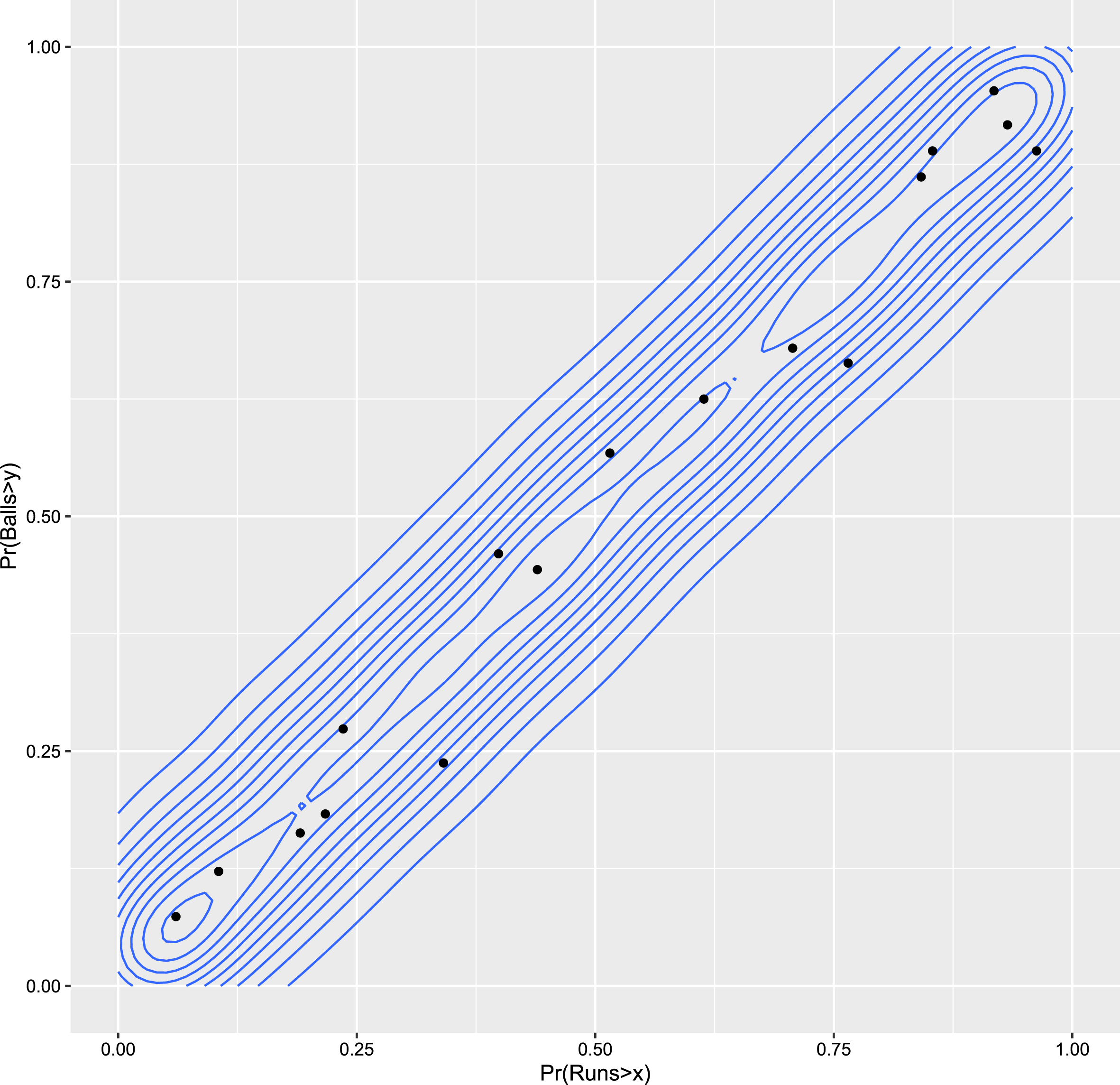
As described in the previous sections, for the 17 ODI opening partnerships shown in Table 1, the joint survival distribution of runs scored and balls faced is modeled using gamma marginals and the Frank copula. The parameter estimates of this model are derived by maximizing the likelihood function in Equation (6). For example, the MLEs for the bivariate joint distribution for the opening partnership pair Dhawan S and Rahane A M are
Fig. 1
Contour plot for the joint survival probability distribution obtained using gamma marginals and Frank copula for the partnership between Dhawan D and Rahane A M.
For the purpose of exploring the performance of partnerships, we define five different stages of the game of which we believe crucial for evaluating partnerships. For each case, we have estimated the joint survival probability for scoring more than specific number of runs and facing more than specific number of balls.
1 Case 1: Survive scoring more than 45 runs and facing more than 30 balls (Table 3)
2 Case 2: Survive scoring more than 50 runs and facing more than 60 balls (Table 3)
3 Case 3: Survive scoring more than 60 runs and facing more than 60 balls (Table 4)
4 Case 4: Survive scoring more than 75 runs and facing more than 60 balls (Table 4)
5 Case 5: Survive scoring more than 100 runs and facing more than 90 balls (Table 5)
Table 3
Marginal and joint survival probabilities for runs scored and balls faced of partnerships case 1 and case 2
| Case 1 | Case 2 | |||||||
| Partnership | P(R > 45) | P(B > 30) | P(R > 45, B > 30) | Rank | P(R > 50) | P(B > 60) | P(R > 50, B > 60) | Rank |
| Amla H M and de Kock Q | 0.4117 | 0.5983 | 0.4114 | 5 | 0.3777 | 0.3526 | 0.3359 | 5 |
| Bairstow J M and Roy J J | 0.4522 | 0.5811 | 0.4508 | 3 | 0.4278 | 0.3656 | 0.3584 | 3 |
| Cook A N and Bell I R | 0.3630 | 0.5749 | 0.3626 | 11 | 0.3300 | 0.3286 | 0.2988 | 8 |
| Dhawan S and Rahane A M | 0.5415 | 0.7369 | 0.5415 | 1 | 0.5090 | 0.5144 | 0.4914 | 1 |
| Dilshan T M and Perera M D K | 0.3153 | 0.4234 | 0.3094 | 17 | 0.2851 | 0.1857 | 0.1790 | 17 |
| Fakhar Z and Imam-ul-haq | 0.4629 | 0.6700 | 0.4627 | 2 | 0.4351 | 0.4544 | 0.4180 | 2 |
| Haddin B J and Watson S R | 0.3724 | 0.5778 | 0.3713 | 9 | 0.3364 | 0.2904 | 0.2716 | 10 |
| Jayawardene D P M and Dilshan T M | 0.4389 | 0.6305 | 0.4364 | 4 | 0.3974 | 0.3265 | 0.3102 | 6 |
| McCullum B B and Ryder J D | 0.3800 | 0.5433 | 0.3768 | 8 | 0.3515 | 0.2766 | 0.2630 | 12 |
| McCullum and Guptill M J | 0.3297 | 0.4332 | 0.3203 | 16 | 0.3001 | 0.1890 | 0.1809 | 16 |
| Sharma R G and Dhawan S | 0.4115 | 0.6220 | 0.4110 | 6 | 0.3784 | 0.3594 | 0.3363 | 4 |
| Smith G C and Amla H M | 0.3433 | 0.5407 | 0.3429 | 14 | 0.3082 | 0.2927 | 0.2705 | 11 |
| Sarkar S and Iqbal T | 0.3324 | 0.5209 | 0.3316 | 15 | 0.3000 | 0.2684 | 0.2499 | 14 |
| Tendulkar S R and Sehwag V | 0.3731 | 0.5075 | 0.3705 | 10 | 0.3413 | 0.2587 | 0.2512 | 13 |
| Tharanga W U and Dilshan T M | 0.3600 | 0.5207 | 0.3586 | 13 | 0.3312 | 0.2926 | 0.2761 | 9 |
| Warner D A and Finch A J | 0.3995 | 0.5618 | 0.3988 | 7 | 0.3673 | 0.3187 | 0.3082 | 7 |
| Shewag V and Gambhir G | 0.3634 | 0.5305 | 0.3620 | 12 | 0.3282 | 0.2496 | 0.2413 | 15 |
Table 4
Marginal and joint survival probabilities for runs scored and balls faced of partnerships case 3 and case 4
| Case 3 | Case 4 | |||||||
| Partnership | P(R > 60) | P(B > 60) | P(R > 60, B > 60) | Rank | P(R > 75) | P(B > 60) | P(R > 75, B > 60) | Rank |
| Amla H M and de Kock Q | 0.3185 | 0.3526 | 0.3047 | 4 | 0.2477 | 0.3526 | 0.2450 | 5 |
| Bairstow J M and Roy J J | 0.3846 | 0.3656 | 0.3470 | 3 | 0.3304 | 0.3656 | 0.3172 | 3 |
| Cook A N and Bell I R | 0.2736 | 0.3286 | 0.2625 | 8 | 0.2076 | 0.3286 | 0.2049 | 10 |
| Dhawan S and Rahane A M | 0.4502 | 0.5144 | 0.4471 | 1 | 0.3753 | 0.5144 | 0.3750 | 1 |
| Dilshan T M and Perera M D K | 0.2340 | 0.1857 | 0.1692 | 17 | 0.1753 | 0.1857 | 0.1455 | 17 |
| Fakhar Z and Imam-ul-haq | 0.3857 | 0.4544 | 0.3805 | 2 | 0.3242 | 0.4544 | 0.3231 | 2 |
| Haddin B J and Watson S R | 0.2749 | 0.2904 | 0.2452 | 11 | 0.2037 | 0.2904 | 0.1942 | 12 |
| Jayawardene D P M and Dilshan T M | 0.3252 | 0.3265 | 0.2840 | 7 | 0.2400 | 0.3265 | 0.2272 | 7 |
| McCullum B B and Ryder J D | 0.3020 | 0.2766 | 0.2484 | 10 | 0.2424 | 0.2766 | 0.2176 | 8 |
| McCullum and Guptill M J | 0.2496 | 0.1890 | 0.1715 | 16 | 0.1909 | 0.1890 | 0.1502 | 16 |
| Sharma R G and Dhawan S | 0.3209 | 0.3594 | 0.3045 | 5 | 0.2517 | 0.3594 | 0.2476 | 4 |
| Smith G C and Amla H M | 0.2488 | 0.2927 | 0.2361 | 13 | 0.1811 | 0.2927 | 0.1783 | 14 |
| Sarkar S and Iqbal T | 0.2452 | 0.2684 | 0.2238 | 15 | 0.1822 | 0.2684 | 0.1759 | 15 |
| Tendulkar S R and Sehwag V | 0.2863 | 0.2587 | 0.2380 | 12 | 0.2214 | 0.2587 | 0.2040 | 11 |
| Tharanga W U and Dilshan T M | 0.2815 | 0.2926 | 0.2549 | 9 | 0.2223 | 0.2926 | 0.2133 | 9 |
| Warner D A and Finch A J | 0.3114 | 0.3187 | 0.2870 | 6 | 0.2444 | 0.3187 | 0.2385 | 6 |
| Shewag V and Gambhir G | 0.2682 | 0.2496 | 0.2251 | 14 | 0.1988 | 0.2496 | 0.1849 | 13 |
Table 5
Marginal and joint survival probabilities for runs scored and balls faced of partnerships case 5
| Case 5 | ||||
| Partnership | P(R > 100) | P(B > 90) | P(R > 100, B > 90) | Rank |
| Amla H M and de Kock Q | 0.1640 | 0.2071 | 0.1528 | 4 |
| Bairstow J M and Roy J J | 0.2604 | 0.2340 | 0.2181 | 3 |
| Cook A N and Bell I R | 0.1324 | 0.1876 | 0.1218 | 8 |
| Dhawan S and Rahane A M | 0.2783 | 0.3533 | 0.2762 | 1 |
| Dilshan T M and Perera M D K | 0.1099 | 0.0820 | 0.0625 | 17 |
| Fakhar Z and Imam-ul-haq | 0.2456 | 0.3091 | 0.2396 | 2 |
| Haddin B J and Watson S R | 0.1241 | 0.1404 | 0.0968 | 13 |
| Jayawardene D P M and Dilshan T M | 0.1437 | 0.1589 | 0.1114 | 10 |
| McCullum B B and Ryder J D | 0.1705 | 0.1385 | 0.1145 | 9 |
| McCullum and Guptill M J | 0.1239 | 0.0826 | 0.0638 | 16 |
| Sharma R G and Dhawan S | 0.1693 | 0.2035 | 0.1520 | 5 |
| Smith G C and Amla H M | 0.1074 | 0.1585 | 0.0971 | 12 |
| Sarkar S and Iqbal T | 0.1124 | 0.1380 | 0.0932 | 14 |
| Tendulkar S R and Sehwag V | 0.1458 | 0.1320 | 0.1070 | 11 |
| Tharanga W U and Dilshan T M | 0.1522 | 0.1672 | 0.1279 | 7 |
| Warner D A and Finch A J | 0.1648 | 0.1812 | 0.1446 | 6 |
| Shewag V and Gambhir G | 0.1215 | 0.1138 | 0.0865 | 15 |
Case 1 represents surviving in the innings to score more than 45 runs and facing more than 30 balls (5 overs), which can be considered as minimum reasonable performance by an opening pair. Results of this case are shown in Table 3. The partnership pair Dhawan S and Rahane A M has been ranked the top in the list in terms of the joint survival probability (0.54).
Case 2, case 3, and case 4 can be considered as well-founded partnerships in ODI cricket as these last more than 60 balls (10 overs) with decent scores of 50 runs, 60 runs, and 75 runs, respectively. Moreover, the strengths of the effectiveness of these partnerships increase as it moves from case 2 through case 4. In ODI cricket, it is a known strategy for the bowling team to put all their efforts to dismiss at least one partner (if not both) of the opening pair during the first 10 overs (powerplay). On the other hand, inability to accomplish that may be considered a weakness of the bowling team, which consequently lowers the bowlers’ confidence. Given that, case 4 provides more confidence to the other top order and to the middle order batsmen as they continue to build the innings to go for a higher total. Case 5 represents scoring more than 100 runs and batting more than 15 overs (90 balls), which gives an impressive foundation to the innings of the batting team.
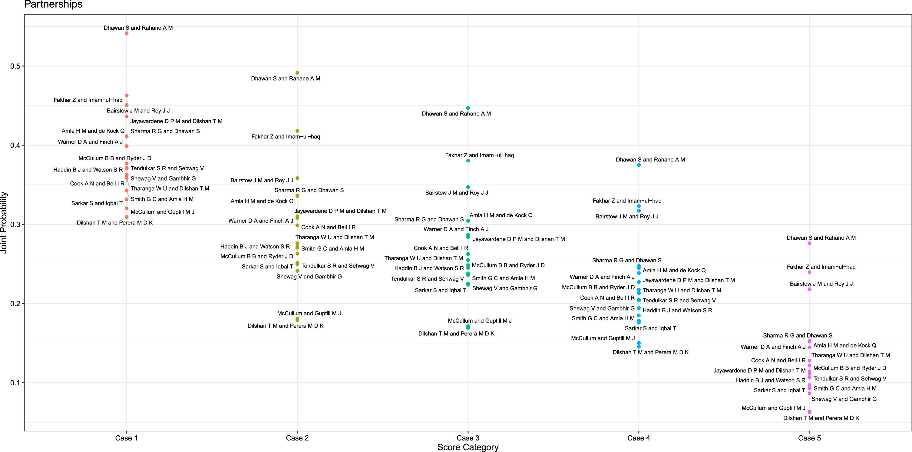
It is interesting to notice that Dhawan S & Rahane A M have the highest joint survival probability in all five cases. Also note that the second and the third highest joint probabilities for surviving in all five cases are recorded by the same partnership pairs: Fakhar Z & Imam-ul-haq, and Bairstow J M & Roy J J, respectively. These results indicate that these two pairs are consistently better than the other partnership pairs considered in this study. Graphical representation of the above cases for all the partnerships considered in this study is shown in Fig. 2. Note that the probabilities are steadily decreasing as the cases move from case 1 to case 5; this is because of moving from case 1 to case 5 the chance of surviving for an opening pair goes down.
Fig. 2
Joint probabilities of partnerships for different cases.
4.2Individual T20 batting performance
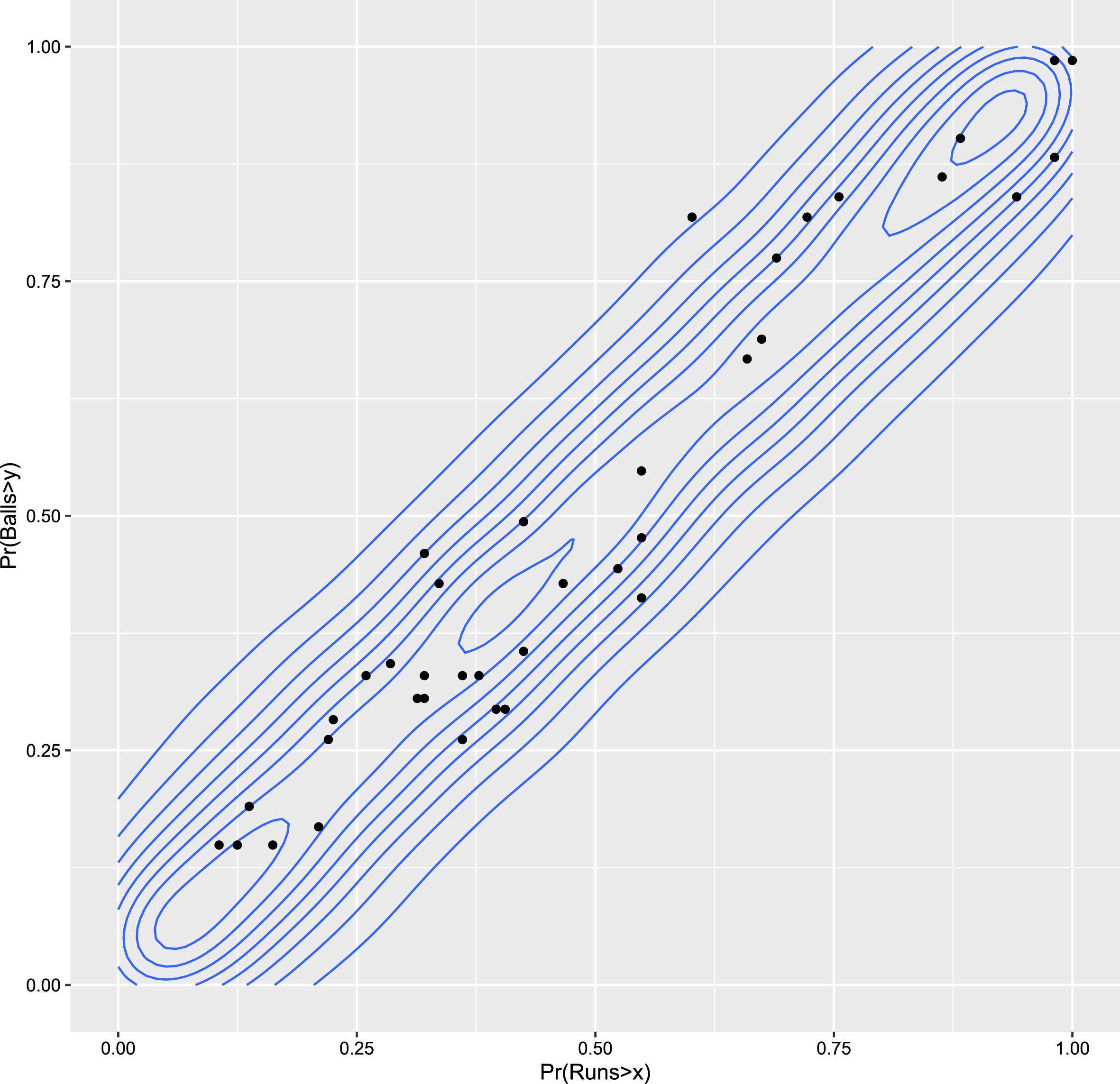
Similar to the partnership analysis, the runs scored and balls faced by T20 batsmen in Table 2 were modeled using gamma marginals and Frank copula. The parameters of the model were estimated by maximizing the likelihood function in Equation (6). For example, the MLEs for the Pakistan top order batsman, Babar Azam were
Fig. 3
Contour plot for the joint survival probability distribution obtained using gamma marginals and Frank copula for T20 batsman Babar Azam.
To evaluate the individual batting performance using the joint survival distribution, we considered 13 different cases based on different stages of the innings. We used the notation (r, b) to represent the case scoring more than r runs by surviving more than b balls. For example, the notation (20,30) indicates the case of scoring more than 20 runs while surviving more than 30 balls. The thirteen different cases for individual batting performance and their respective joint probabilities are shown in Fig. 4.
Fig. 4
Individual player performance.
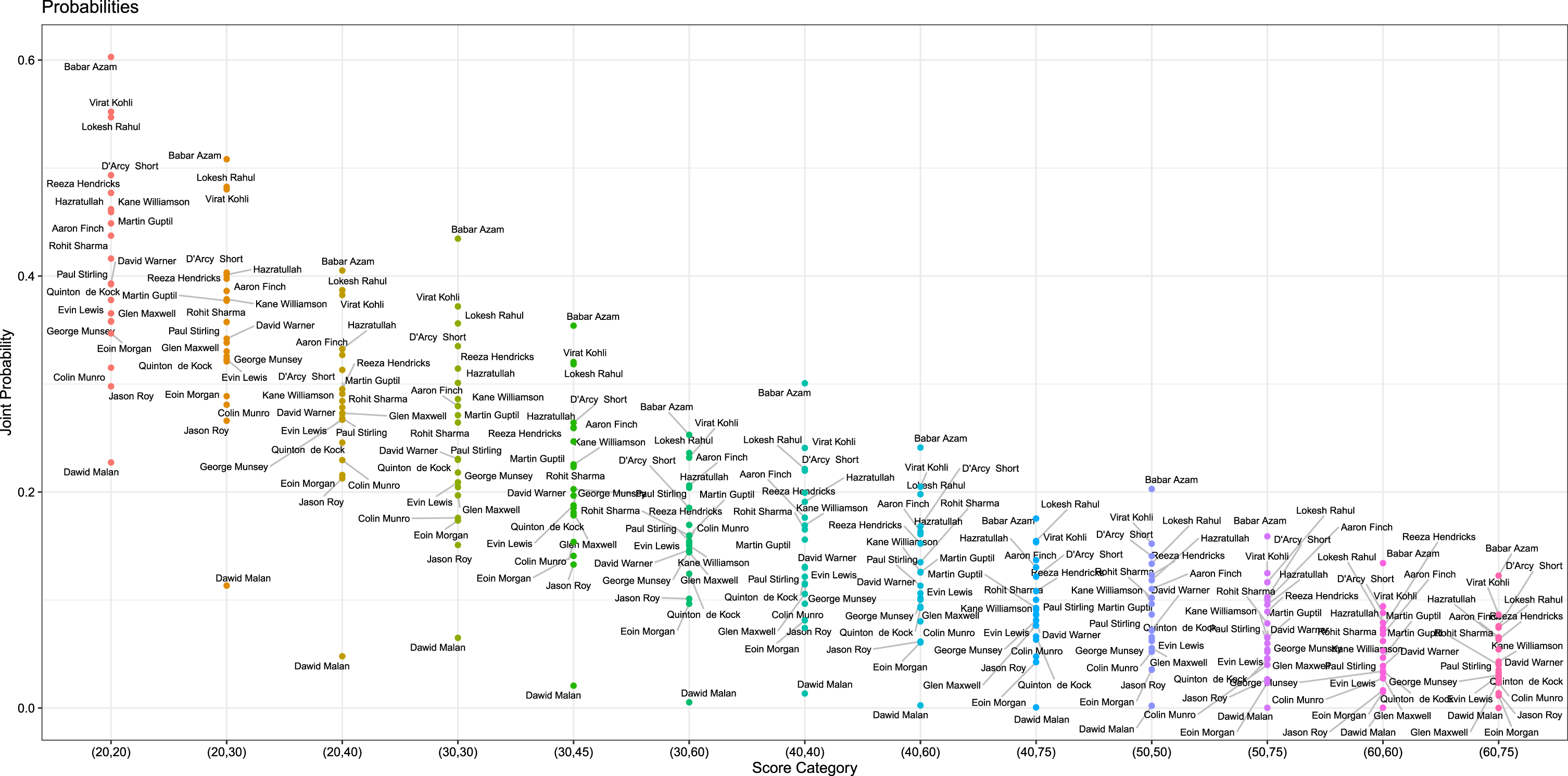
Pakistan top order batsman Babar Azam had the highest joint survival probability in all thirteen categories. Interestingly, according to the ICC T20 batsmen ranking as of July 2020, Babar Azam was also the top ranking T20 batsman. Another interesting observation is that Virat Kohli who was the 10th ranking (based on ICC ranking) batsman has been occupying the number 2 rank in 9 cases and number 3 rank in 4 cases in the joint survival probability list for the thirteen cases. Lokesh Rahul who was the second ranking (based on ICC ranking) batsman in our data set, has been occupying ranks number 2 in 4 cases, rank number 3 in 6 cases, and rank number 4 in 3 cases in our joint survival probability ranking. In this study, we particularly focused on the batsman’s ability to survive in different conditions in the game than evaluating the aggressiveness of scoring runs. Nevertheless, the results in the study fairly match with the ICC T20 batsmen ranking, which indicates that the ICC batsmen ranking system is an effective tool to evaluate the performance of batsmen in cricket.
5Conclusions
Copula applications are common in the fields such as finance and reliability engineering; nevertheless, in sports literature, copula applications are limited. In this article, we have shown the effectiveness of copula methods as an application to the game of cricket. As the main contribution of this study, we were able to model the bivariate joint distribution of the number of runs scored and the number of balls faced using copula functions for the partnerships in ODI cricket and individual batsmen in T20 cricket. Furthermore, these bivariate distributions were used to rank the batting performance of the opening partnerships as well as the batting performance of individual T20 batsmen for different stages in the game.
Based on the joint survival probability estimates, the partnership pair, Dhawan S & Rahane A M, have been ranked the top in all the five partnership cases considered in this study. The second and the third highest joint survival probabilities in all five cases were recorded by the partnership pairs: Fakhar Z & Imam-ul-haq, and Bairstow J M & Roy J J, respectively. These results indicated that above three partnership pairs were consistently better than the other partnership pairs considered in this study.
Babar Azam, who is number one in the ICC T20 batsmen ranking, has been ranked first based on the joint survival probability approach. Furthermore, Virat Kohli and Lokesh Rahul were ranked as the next two highest ranking T20 batsmen with respect to the thirteen joint survival probability cases we considered. It is important to note that the probability based ranking method proposed in this study closely complies with the ICC batting ranking. Nevertheless, there are some noticeable deviations between the two ranking approaches, for example, Virat Kohli is in the tenth place in the ICC ranking; however, he has been ranked as the second or the third from joint survival probability approach.
We believe that the results of this paper would be useful for team managers. In particular, they can use the proposed method to select the best opening pair or individual batsmen from a pool of players for a given match. Furthermore, in this study, copula applications are shown to be a useful tool to evaluate player performance in the game of cricket, and thus, this article may bring attention to the area and open up opportunities for future research. As a future extension, we are expecting to apply a similar approach to evaluate the bowling performance in cricket. In addition, another interesting future research would be to expand for multivariate approach considering other performance indicators such as the number of fours, number of sixes, and number of dot balls.
References
1 | Balakrishnan, N. , & Lai, C. D. , (2009) . Continuous Bivariate Distributions, Springer Science & Business Media, New York, NY. |
2 | Bhattacharjee, D. , Lemmer, H. H. , Saikia, H. , & Mukherjee, D. , (2018) . Measuring performance of batting partners in limited overs cricket, South African Journal for Research in Sport, Physical Education and Recreation 40: , 1–12. |
3 | Boshnakov, G. , Kharrat, T. , & McHale, I. G. , (2017) . A bivariate Weibull count model for forecasting association football scores, International Journal of Forecasting 33: , 458–466. |
4 | Clayton, D. G. , (1978) . A model for association in bivariate life tables and its application in epidemiological studies of familial tendency in chronic disease incidence, Biometrika 65: , 141–151. |
5 | Das, S. , 2011. On generalized geometric distributions: Application to modeling scores in cricket and improved estimation of batting average in light of notout innings, IIM Bangalore Research Paper. |
6 | Frank, M. J. , (1979) . On the simultaneous associativity of F(x, y) and x + y - F(x, y), Aequationes Mathematicae 19: , 194–226. |
7 | Gumbel, E. J. , (1960) . Distributions des valeurs extremes en plusiers dimensions, Publ Inst Statist Univ Paris 9: , 171–173. |
8 | Joe, H. , & Xu, J. J. , (1996) . The estimation method of inference functions for margins for multivariate models, Technical report, University of British Columbia, Department of Statistics. |
9 | Kim, J.-M. , Baik, J. , & Reller, M. , 2019. Control charts of mean and variance using copula markov SPC and conditional distribution by copula, Communications in Statistics-Simulation and Computation pp. 1-18. |
10 | McHale, I. , & Scarf, P. , (2007) . Modelling soccer matches using bivariate discrete distributions with general dependence structure, Statistica Neerlandica 61: , 432–445. |
11 | Nelsen, R. B. , (1999) . An Introduction to Copulas, Springer-Verlag New York, Inc., New York, NY. |
12 | RCore Team, 2018. R: A Language and Environment for Statistical Computing, R Foundation for Statistical Computing, Vienna, Austria. URL: https://www.R-project.org/ |
13 | Scarf, P. , Shi, X. , & Akhtar, S. , (2011) . On the distribution of runs scored and batting strategy in test cricket, Journal of the Royal Statistical Society: Series A (Statistics in Society) 174: , 471–497. |
14 | Sklar, M. , (1959) . Fonctions de repartition an dimensions et leurs marges, Publ Inst Statist Univ Paris 8: , 229–231. |
15 | Swartz, T. B. , Gill, P. S. , & Muthukumarana, S. , (2009) . Modelling and simulation for one-day cricket, Canadian Journal of Statistics 37: , 143–160. |
16 | Talukdar, P. , (2020) . Investigating the role of opening partners while chasing on the outcome of twenty20 cricket matches, Management and Labour Studies 45: , 222–232. |
17 | Tavassolipour, M. , Karimian, M. , & Kasaei, S. , (2013) . Event detection and summarization in soccer videos using Bayesian network and copula, IEEE Transactions on Circuits and Systems for Video Technology 24: , 291–304. |
18 | Valero, J. , & Swartz, T. B. , (2012) . An investigation of synergy between batsmen in opening partnerships, Sri Lankan Journal of Applied Statistics 13: , 87–98. |
Appendices
6 Appendix
6.1 Examples of other Archimedean copula types
6.1.1 Clayton copula
The Clayton copula (Clayton 1978) function is expressed as
(9)
6.1.2 Gumbel copula
The Gumbel copula (Gumbel 1960) function can be obtained as
(10)
6.2 Parameter estimates for partnerships and individual batsmen
Tables 6 and 7 show the parameter estimates for the joint survival distribution obtained using gamma marginals with Frank copula for ODI opening partnerships and T20 individual batsmen, respectively.
Table 6
Parameter estimates for the joint survival distribution obtained from Gamma Marginals and Frank copula for ODI opening partnerships
| Partnerships | αx | βx | αy | βy | ξ |
| Amla H M and de Kock Q | 0.81 | 66.56 | 1.03 | 55.44 | 25.43 |
| Bairstow J M and Roy J J | 0.51 | 154.93 | 0.83 | 74.08 | 25.74 |
| Cook A N and Bell I R | 0.76 | 62.00 | 1.01 | 53.21 | 22.67 |
| Dhawan S and Rahane A M | 0.87 | 90.28 | 1.18 | 71.66 | 34.40 |
| Dilshan T M and Perera M D K | 0.66 | 62.30 | 0.95 | 37.43 | 19.53 |
| Fakhar Z and Imam-ul-haq | 0.62 | 116.66 | 0.97 | 79.48 | 27.20 |
| Haddin B J and Watson S R | 0.88 | 53.03 | 1.31 | 36.83 | 18.68 |
| Jayawardene D P M and Dilshan T M | 1.14 | 46.19 | 1.50 | 34.78 | 16.51 |
| McCullum B B and Ryder J D | 0.60 | 89.26 | 1.13 | 41.19 | 17.49 |
| McCullum and Guptill M J | 0.64 | 68.87 | 0.99 | 36.37 | 16.91 |
| Sharma R G and Dhawan S | 0.77 | 70.72 | 1.18 | 48.69 | 21.90 |
| Smith G C and Amla H M | 0.85 | 50.77 | 1.00 | 48.96 | 23.68 |
| Sarkar S and Iqbal T | 0.74 | 57.82 | 1.02 | 44.68 | 21.91 |
| Tendulkar S R and Sehwag V | 0.72 | 68.62 | 0.99 | 44.71 | 21.27 |
| Tharanga W U and Dilshan T M | 0.61 | 81.54 | 0.86 | 57.38 | 21.73 |
| Warner D A and Finch A J | 0.74 | 72.61 | 0.98 | 53.65 | 24.84 |
| Shewag V and Gambhir G | 0.85 | 54.07 | 1.24 | 35.11 | 21.02 |
Table 7
Parameter estimates for the joint survival distribution obtained from Gamma Marginals and Frank copula for T20 individual batsmen
| Batsman | αx | βx | αy | βy | ξ |
| Babar Azam | 1.06 | 41.33 | 1.63 | 20.32 | 22.16 |
| Virat Kohli | 1.04 | 39.77 | 1.59 | 18.11 | 20.27 |
| D’Arcy Short | 0.83 | 42.43 | 1.36 | 20.27 | 18.87 |
| Lokesh Rahul | 1.03 | 40.87 | 1.72 | 16.07 | 21.26 |
| Aaron Finch | 0.69 | 55.49 | 1.16 | 20.27 | 24.61 |
| Hazratullah | 0.72 | 54.61 | 1.32 | 19.42 | 13.37 |
| Reeza Hendricks | 0.84 | 39.86 | 1.39 | 18.76 | 20.13 |
| Rohit Sharma | 0.75 | 42.51 | 1.11 | 20.54 | 21.39 |
| Kane Williamson | 0.97 | 33.16 | 1.52 | 16.07 | 16.90 |
| Martin Guptil | 0.87 | 37.87 | 1.55 | 15.10 | 17.11 |
| Paul Stirling | 0.65 | 48.81 | 1.33 | 15.68 | 20.43 |
| David Warner | 0.78 | 41.26 | 1.31 | 16.13 | 14.96 |
| George Munsey | 0.70 | 45.88 | 1.18 | 16.34 | 18.57 |
| Evin Lewis | 0.56 | 59.58 | 1.30 | 15.26 | 16.51 |
| Quinton de Kock | 0.83 | 35.27 | 1.27 | 16.09 | 15.89 |
| Glen Maxwell | 0.76 | 42.79 | 1.29 | 14.74 | 18.34 |
| Colin Munro | 0.62 | 46.68 | 1.05 | 16.80 | 15.97 |
| Jason Roy | 0.66 | 40.34 | 1.24 | 13.40 | 17.77 |
| Eoin Morgan | 0.83 | 31.97 | 1.63 | 11.45 | 15.05 |
| Dawid Malan | 1.68 | 9.54 | 2.23 | 7.25 | 10.75 |


