
Misadventures in Monte Carlo
Abstract
Estimating probability is the very core of forecasting. Increasing computing power has enabled researchers to design highly intractable probability models, such that model results are identified through the Monte Carlo method of repeated stochastic simulation. However, confidence in the Monte Carlo identification of the model can be mistaken for accuracy in the underlying model itself. This paper describes simulations in a problem space of topical interest: basketball season forecasting. Monte Carlo simulations are widely used in sports forecasting, since the multitude of possibilities makes direct calculation of playoff probabilities infeasible. Error correlation across games requires due care, as demonstrated with a realistic multilevel basketball model, similar to some in use today. The model is built separately for each of 20 NBA seasons, modeling team strength as a composition of player strength and player allocation of minutes, while also incorporating team persistent effects. Each season is evaluated out-of-time, collectively demonstrating systematic and substantial overconfidence in playoff probabilities, which can be eliminated by incorporating error correlation. This paper focuses on clarifying the use of Monte Carlo simulations for probability calculations in sports.
1Introduction
Estimating probability is the very core of forecasting. Increasing computing power has enabled researchers to design highly intractable probability models, such that the model results are identified through the Monte Carlo method of repeated stochastic simulation. As described in the seminal paper on the topic, “if we assume that the probability of each possible event is given, we can then play a great number of games of chance, with chances corresponding to the assumed probability distributions” (Metropolis and Ulam 1949). Every event in a sequence of trials is determined randomly, with odds determined by estimated probabilities, and then results are tallied. When repeated many times this provides an estimate of the properties of the sequence in question. However, highly confident estimates from the Monte Carlo procedure can be mistaken for accuracy in the underlying probabilities themselves. Issues of this nature have gained significant public prominence most recently through election forecasting, of which Andrew Gelman stated “we ignored correlations in some of our data, thus producing illusory precision in our inferences” (Gelman 2016). This paper describes simulations in another problem space of topical interest: basketball season forecasting.
The question of whether or not a team will make the playoffs is relevant to many people. It is of interest to team personnel who wish to accurately understand their team, to the large sports betting market where significant sums are wagered, to academics who seek to apply statistical methods to these questions, and to the multitude of fans who seek to debate the quality of their teams. In sports forecasting, Monte Carlo simulations are widely used, such as by FiveThirtyEight (Boice 2015), Football Outsiders (Harris 2008), FanGraphs (Agami and Walsh 2013), and Nylon Calculus (Restifo 2016), among others. These models predict each game individually, rather than directly modeling which teams will make the playoffs. Doing so has the advantage of addressing many other quantitative questions about the season, including who will win any particular game. Even with outcome probabilities for every regular season game, the multitude of possibilities makes direct calculation of playoff probabilities infeasible. As such, simulating the season, and doing so many times, provides a reasonable estimate. However, many practitioners fall prey to erroneous use of the Monte Carlo method. In the model setup demonstrated in this paper, uncertainty in our parameters needs to be accounted for when making inferences about the future. This paper explains the theoretical underpinnings of Monte Carlo simulations and basketball models, and then demonstrates the problem in detail by designing a realistic basketball model. This model is similar to some in use today in terms of its multilevel structure, but largely different in its treatment of correlation. The model is built separately ahead of each of 22 NBA seasons and evaluated on each out-of-time, demonstrating systematic and substantial overconfidence in playoff probabilities when it is simulated without accounting for variance.
The model demonstrated in this paper addresses a different problem than most other approaches in preceding papers. Topics that are well-covered in the basketball literature on win probability include attribution of wins to players, evaluating team strength metrics for existing teams or predicting game results using in-season information, and testing the efficiency of market odds.
Manner (2016) uses the first half of an NBA season to predict the subsequent half, and is interested in the effectiveness of quantitative models against market odds. Likewise, Loeffelholz et al. (2009) use the first part of a season to predict the remainder, and compare against expert opinion. Ruiz and Perez-Cruz (2015) use the course of the NCAA season to predict its final tournament. None of those papers need to model minute allocation for previously unobserved team compositions, unlike this paper.
Berri (1999), Ángel Gómez et al. (2008), and Page et al. (2007) are among a literature that examines which in-game statistics best correlate with winning, to decompose which player or team talents are the most crucial. Barrow et al. (2013) compare different methods of team strength, using 20-fold cross validation as their criteria. Štrumbelj and Vrača (2012) use the four factors (team and opponent statistics for shooting, turnovers, rebounding, and free throws) to forecast team win probability. The model developed in this paper does not decompose the attributes of player talent, but instead uses overall player quality to identify the strength of teams.
Vaz de Melo et al. (2012) is similar to this paper in that it predicts the results of an entire season based on data prior to that season. It validates results on the model built across all of its sample, differing from this paper which generates separate models ahead of every season. They build models purely on network effects, with a method that generalizes to any sport. They generate and evaluate an ordering of teams rather than specific probabilities.
This paper contributes to the literature of basketball models by predicting an entire season of play only using data available before a season, composing a multilevel model that models team strength as a composition of player strength and player allocation of minutes, while also incorporating team persistent effects. Much of the prior research relies on in-season information, such that team strength and player allocation are largely already known. This paper is concerned with the accuracy, and not simply the rank-order, of playoff likelihood, and focuses on clarifying the use of Monte Carlo simulations for such calculations in sports.
This topic is approached in this paper through incremental detail in subsequent sections. Section 2 describes the fundamental problem using a coin flip example. Section 3 introduces the issue in sports modeling, describing the types of correlation that can emerge in sports and how other models have approached them. Section 4 structures, builds, and evaluates a reasonable basketball model that provides accurate playoff probabilities when the Monte Carlo procedure is used with variance propagation.
2Classic coin flip demonstration
Suppose we have in our possession a fair coin. When you toss a coin once, it will be heads 100% or 0% of the time, since it will land either heads or tails, respectively. However by the time you have tossed a coin, say, 82 times, you are likely to have seen close to 50% heads. We can quantify with the binomial cumulative distribution function (CDF) that there is nearly an 88% chance that we will observe +/- 5 of the expected average of 41 heads. The more times we flip the coin, the more likely we are to be close to the average value of 50% heads. This is, at its core, the law of large numbers, which clarifies that as more data is available, the resulting average eventually becomes closer to the expected value.
We do not have to derive this coin flip result through a simulation, but simulation will become important in cases where exact distributions are unknown.
This example relies on a perfectly balanced coin. Suppose instead our coin comes from an imprecise coin maker, a mint that tolerates some variation in their coins. The coins are, after all, designed to be used primarily as currency, and their balance is a secondary feature that is probably of little importance—outside of American football, that is.
Let’s suppose that the balance of the coins from this mint follows a normal distribution centred at 50% with a standard deviation of 5%. This means that about 68% of the coins will be between 45% and 55% heads, with 95% of them between 40% and 60%.
These parameters imply that the selected coin is on average fair, but often with some noticeable variation. If we pull a coin from this distribution and flip it 82 times, our expectation for the resulting distribution should be wider than if we used the perfectly fair coin, because we do not know the balance of our coin ahead of time. Some of the time we will get a coin with a near perfect balance of 50%, giving the results we saw earlier. However we will often get a coin with a 48% probability of heads, or 52% probability of heads, or any non-discrete number from this distribution. Crucially, the variation results in error correlation in any given coin flipping session.
If we incorrectly assumed the coin selected will always be fair, with long enough sessions we would incorrectly expect each session to almost always converge to nearly 50% heads and 50% tails. However, if we account for the possibility of an unbalanced coin, we should realize that converging to something other than 50% heads in a given session is very reasonable.
In this scenario we have a mixture distribution, where the outcome of our coin flip is a random variable that is contingent on which coin was selected for flipping, which is another random variable. Similar to our example, mixture models have been explained using the example of a small selection of coins to choose from (Do and Batzoglou 2008; Choudhury 2010).
If we overlay 100,000 simulations of a fair coin with 100,000 simulations of the mixture distribution, we can see the variance differences in Fig. 1.
Fig.1
Difference in sampled distributions
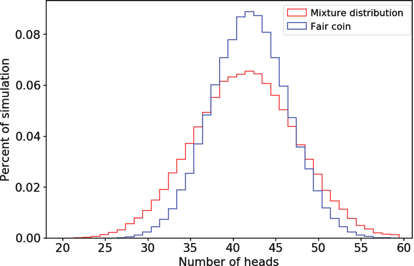
Both are symmetrical, with mean, median, and mode of 41. The mixture distribution is much more dispersed. We are now much less likely to see heads within 41 +/- 5, and much more likely to see extreme values of heads. Our point estimate of the number of heads in a session of 82 coin flips is still 41, but that estimate now has higher variance, visible in much thicker tails and less central mass.
3Application to predictions in professional sports
3.1Intuitive description
Readers with an interest in sports are likely to have deduced the meaning behind 82 coin flips. 82 is the length of a National Basketball Association (NBA) or National Hockey League (NHL) regular season (top professional leagues in their respective sports). Let’s apply our insight about Monte Carlo simulations to a simplified model of the NBA before discussing more realistic cases.
Suppose we wanted to predict playoff probabilities for the Cleveland Cavaliers ahead of the 2016-17 season. Presume they play 82 games against a constant average opponent. For the moment we shall disregard variance in opponent quality, the NBA’s sizable home court advantage, and other factors that result in unequal win probabilities across games. We could believe that the Cleveland Cavaliers are a strong team with a 70% win probability in each game, whereby we expect them to win around 57 games in the season. This is not an implausible estimate of their team quality given that it is the bounty of wins they achieved in the season prior.
However, we cannot be sure that Cleveland will actually be that good. Perhaps they will be better, perhaps they will be worse. The team could suffer unfortunate injuries. If we add a standard deviation of 5% around the team’s per-game win probability, suddenly their win distribution becomes much wider. These two distributions are shown in Fig. 2.
Fig.2
Cleveland win distribution with and without team quality uncertainty.
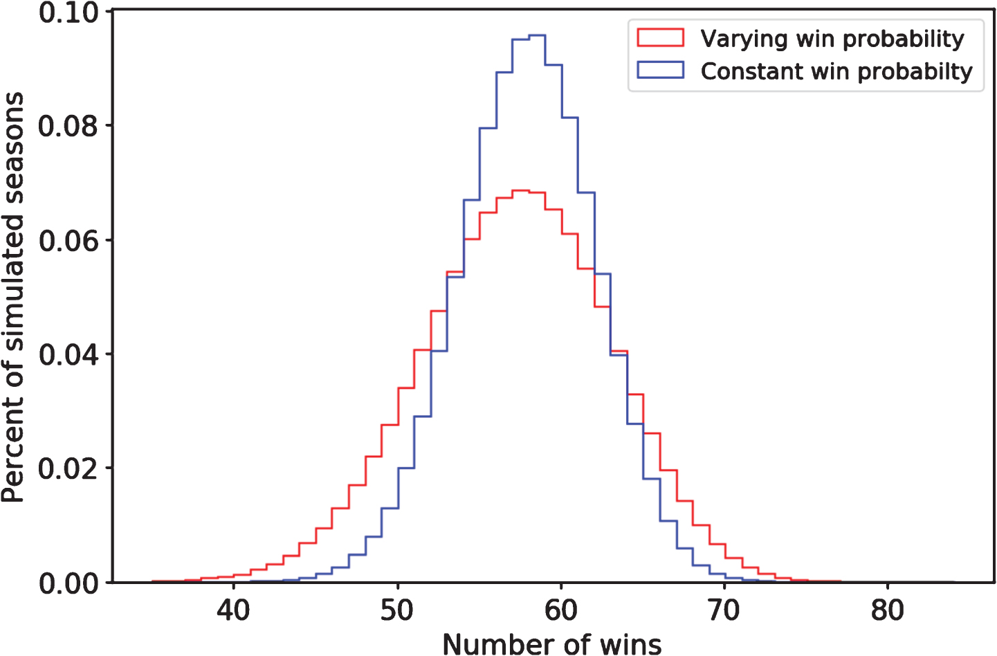
Let’s continue with simplifying assumptions and presume it takes 44 wins to make the playoffs, as it did in the prior year. What is the probability of Cleveland making the playoffs? In both models, on average, we expect the Cavaliers to comfortably make the playoffs, with 57 wins. In the model that does not account for variance, they make the playoffs about 99.9% of the time. In the model with a bit of variance, it’s only about 98.1%. That might not seem like a big difference, but it’s a 15-fold increase in the odds of them missing the playoffs.
In most studies involving mixture distributions, the mixture components and their weights are unobserved, such that a “fundamental statistical problem is to estimate the mixing distribution” (Chen et al. 2008). However, in our study we start by modeling the components and then focus on correct inference when mixing them. In our Cleveland Cavalier example, even if the mixture components are known, if a forecaster makes the mistake of not propagating uncertainty, they will also overestimate the probability of the Cavaliers winning their division, winning the conference, advancing to the NBA finals, etc., just as they will underestimate the probability of weak teams doing any of those. Ultimately, the Cleveland Cavaliers did make the playoffs, as we would predict in either case. Given the high level of predictability in the NBA season, many observations may be needed to identify a calibration problem with playoff predictions.
The point is not to suggest that either playoff probability is correctly calculated, nor that the ratio is correct either. This is a vastly simplified example with arbitrary parameters. The point is that in any Monte Carlo simulation, variance in the underlying probabilities needs to be passed through into the simulation itself, or else we are led to thoroughly implausible claims about distributions. In this paper we are concerned with prediction quality entirely outside of the observed prior data, rather than of model fit on historical data or the specific values of parameters. Parameter error and model error correlation matter because “evidence indicates that substantial size distortions may result if one ignores uncertainty about the regression vector” (West 1996). Fitting the data well in-sample does not guarantee a strong fit on out-of-sample data, particularly when the data has time-dependence. Professional sports is one realm where out-of-time distortions are of particular importance, because of the monetary sums wagered on future performance and the public interest in predicting future team success.
3.2The effect of error correlation on variance
A lack of independence between observations can have drastic consequences for models, including variance mis-estimation for the predictions and the coefficients (Diebold and Mariano 2002; Dunlop 1994). We can apply this insight to basketball models in a simplified example across two games with correlated errors. Using a very simple model of team quality, we will demonstrate how error correlation can lead to increased variance.
In game outcomes, positive correlation could come from many factors, such as injuries, fatigue, or any streakiness associated with player or team performance. Teams could discover an unpredictably talented rookie. A team with substantial roster turnover could find their players complement each other’s skills better or worse than could have been forecasted. Players could be suspended due to events during the season, unknown before the season. A stochastic set of losses could push a team out of playoff contention, leading them to trade away quality players and causing future losses. For all of these reasons, our hypothesis is that correlation is positive. There are also reasons why correlation could be negative, such as losing games galvanizing teams to find ways to win, or winning teams resting players since they are already winning enough games. However, we expect that these are outweighed by the sources of positive correlation. Teams usually have strong incentives to maximize their wins at all points in the season.
Let X1 and X2 be a team’s quality in two distinct games, with X1 preceding X2. X1 has mean μ and a stochastic error term ɛ1 ∼ N (0, σ2). X2 also has mean μ, but with an autoregressive error term ɛ2 = ρɛ1 + ω, where ω has the same N (0, σ2) distribution as ɛ1, and ω and ɛ are independent of each other. In this setup μ is our baseline team quality and ρ is the degree of autocorrelation. If the major factor causing correlated errors is among the leading factors listed previously, such as injury, then we could expect a positive ρ term.
Our expectation of average quality for the team across the two-game season is
However, what is the variance of that team average quality? By the definition:
(1)
We derive:
(2)
If ρ = 0 and there is no autocorrelation, the variance is
If true errors are correlated, but the model setup assumes them to be uncorrelated, then variance can be greatly underestimated.
3.3Properties of Monte Carlo simulations
The Monte Carlo simulator is where we take independent draws from a generating function, with the goal of estimating properties of that function, such as its mean. We can calculate the expected value of a function by repeatedly and randomly sampling from its distribution.
For any random variable X with expected value μ and variance σ2, we can use Chebyshev’s inequality to derive a relevant form of the law of large numbers (as shown in Rey-Bellet 2010):
(3)
As n increases, our probability of being off by any given ɛ decreases, meaning that our estimate of
The Monte Carlo method is particularly useful in scenarios where the function in question is intractable and we cannot directly compute its mean, variance, or other statistical properties. Calculating whether a team will make the playoffs in the NBA is one such example, which depends on the outcome of 1,230 games that have different probabilities and may be conditional on each other. Even if they were independent, we would have 21230 possible permutations, making an exact playoff probability calculation infeasible even if we know accurate probabilities for each game. Repeated simulation can be performed efficiently to arrive at close calculations. It was evident, even in 1949, that “modern computing machines are extremely well suited to perform the procedures described” (Metropolis and Ulam 1949).
Suppose that X here is a sequence of 0 or 1 playoff draws indicating whether a particular team makes the playoffs in a given simulation of our playoff function. In the binary case, variance of each Bernoulli selection is p (1 - p), which is maximized at
(4)
Applying this to our Monte Carlo error formula, when considering probabilities:
(5)
Should we, for example, take 10,000 simulations (n = 10, 000), the probability of being more than 1% (ɛ = 0.01) off in our estimate is no greater than 6.25%. Further, should our team of interest have a playoff probability higher or lower than 50%, according to our playoff generating function, then we are much more likely to converge to under 1% error. While Chebyshev’s inequality defines our limits in any form of Monte Carlo simulation, it is not the only result we can use for binomial probabilities. In many cases we can expect even lower likelihood of deviation, using the central limit theorem, which defines the conditions under which averages of a randomly sampled variable will follow a normal distribution. With some restrictions the binomial distribution can be approximated with a normal distribution (Feller 1945). Either way, regardless of the playoff function used, after a small number of Monte Carlo repetitions we are very likely to observe convergence.
The point is worth repeating: with binary outcomes our Monte Carlo simulation will converge quickly whether or not we have a good model behind it. Running more Monte Carlo simulations should not give us more confidence in our model—it just means that we have discovered the properties of our model with more certainty. The model itself can be entirely wrong.
In other words, the Monte Carlo is a garbage-in-garbage-out estimator.
More formally, if the model predicts X′, which differs from the true value of X, then the Monte Carlo estimator is a biased and inconsistent estimator of X. It is biased because its expected value is X′ instead of X, and it is inconsistent because as we increase the number of simulations, the law of large numbers establishes that we are more likely to converge upon a value of X′ than X.
The fallacy of becoming more confident in our model through more Monte Carlo simulations is compounded when we are incorrectly over-confident in our playoff function. The further away we are from a probability of 50%, that is, the more certain our model is that the team in question will make or miss the playoffs, the lower variance that estimate has, and the more quickly the Monte Carlo simulation will converge. If our model is overly certain, not only do we have that false certainty, but we may be additionally over-confident through a highly precise Monte Carlo estimate.
3.4The implausibility of existing models
This is a problem that is emblematic of how predictions are commonly made in the sports analytics community. Quality models are used as inputs for Monte Carlo simulation, but without accounting for the unavoidable error correlation in those models.
In particular, there have been published simulations that every year suggest that multiple teams (including, of course, the aforementioned 2016-17 Cleveland Cavaliers) have a 100% chance of making the playoffs, with several other teams having over a 99% chance of making the playoffs. Likewise with the weakest teams not making the playoffs, even sometimes in 0% of a large number of simulations. 100% and 0% not only violate civilized concepts of probability given model uncertainty, but they feel incorrect.
The example of the Cleveland Cavaliers is apt because they are carried disproportionately by one of the most dominant players in NBA history, LeBron James. Although they have other very good players, in the absence of James they would perhaps be a marginal playoff team, one that could quite plausibly miss the playoffs if they had other bad luck. What are the odds of an injury to LeBron James causing him to miss most of a season? Certainly greater than 0%. These rather unfortunate events do happen occasionally. Take the 2005-06 Houston Rockets, victims of injuries to both Tracy McGrady and Yao Ming, who fell to 34 wins from 51 the year before. Or the 1996-97 San Antonio Spurs, who went from 59 wins to 20 wins due to the absence of David Robinson, former league Most Valuable Player, for almost the entire season.
In Table 1, the effect of losing a key player is demonstrated. In all cases the teams had substantial decreases in wins compared to their prior season and their subsequent season, due to the absence of at least one dominant player who was part of their roster during all three seasons. Within the injured season, when the player was present in more than a handful of games, the team performed much better in those games than in the rest of the season.
Table 1
Effect of key injuries on team wins
| Year | Team | Player | Prior Year | With Player | Without Player | Next Year |
| 1988-89 | BOS | Larry Bird | 57-25 | 2-4 | 40-36 | 52-30 |
| 1996-97 | SAS | David Robinson | 59-23 | 3-3 | 17-59 | 56-26 |
| 2005-06 | HOU | Tracy McGrady | 53-29 | 27-20 | 7-28 | 52-30 |
| 2009-10 | NOH | Chris Paul | 49-33 | 23-22 | 14-23 | 46-36 |
| 2014-15 | OKC | Kevin Durant | 59-23 | 18-9 | 27-29 | 56-27 |
Not only do some existing models make the mistake of not accounting for error correlation, but it is a serious enough error that their predictions may be unusable for evaluating unlikely scenarios. Their point estimates of wins are generally reasonable, but if anyone was to bet on distributional probabilities, such as chances of making the playoffs, chances of winning the division, or chances of winning the championship, they could be using numbers that are substantially and systematically incorrect.
Some forecasters do not make an adjustment for error correlation, while others are not sufficiently detailed enough for observers to know definitively whether they do or not. Absence of details on how correlation is handled is most likely an indication that the problem was not addressed in the calculations. FanGraphs simply states that to “generate the playoff odds [they] simulate each season 10,000 times” (Agami and Walsh 2013). Football Outsiders provides the detail that the “playoff odds report plays out the season 50,000 times. A random draw assigns each team a win or loss for each game. The probability that a team will be given a win is based on an equation which considers the current Weighted [Defense Adjusted Value over Average] ratings of the two teams as well as home-field advantage” (Harris 2008). At Nylon Calculus (now part of FanSided), Nick Restifo states that he “also simulated the season and resulting draft lottery 10,000 times to estimate the range of wins a team may fall into, the percent chance of netting certain draft picks, and the percent chance of breaking certain records” (Restifo 2016).
FiveThirtyEight, which will be evaluated in more detail in Section 4, provides significantly more detail on how they simulate, and are not only aware of the problem, but devise a strategy to counter it. They update team Elo ratings after each simulated game in a simulated season, such that team strength through the season has path dependence. They claim that this is important, and “matters more than you might think,” backing up this paper’s claim that the effect is very substantial in sports (Boice 2015). Their method has both strengths and weaknesses. It implies that team strength is gained and lost through winning and losing, iteratively through games at a rate defined by the Elo formula. This is different than the scenario where a team should be consistently worse or better than expected through an entire season, due to unexpected minute allocations or significant injury.
4Empirical example: Basketball models
4.1A slightly less simplified model of how wins are currently projected
Playoff projections are a common pastime of fans and analysts alike. Intrinsic to being a sports fan is the willingness to debate your opinions against those of your peers. Casual fans can argue the merits of their teams and the respective likelihood of them making the playoffs. Professional bettors participate in a zero-sum (or negative-sum) field in which it is only sensible to participate if they believe their reasoning to be stronger than that of others. Team managers will ultimately be judged on performance, whether their ex-ante reasoning resulted in ex-post success. Analytical fans and statisticians can test out their methodologies on sports, a realm with defined rules, conclusive outcomes, and suitable randomness. Predicting the collective results of a season, which encompasses the question of which teams make the playoffs, is a metric of how astute our reasoning can be. A common approach to predicting the playoffs is to predict each game in the regular season, across all the teams, and then use Monte Carlo simulations to evaluate how the standings are likely to turn out.
We have strong metrics of player quality, based primarily on prior quality and aging, which correlate well with wins and have season-over-season predictability (as demonstrated in the models in this paper). We also have good accuracy in predicting player minutes. These are the salient features of current strong NBA models (see the discussion at Association for Professional Basketball Research 2016). This is by no means limited to NBA analysis, but it is a particularly demonstrative case. A team’s quality can be represented by the sum of its players’ qualities, weighted by how much time they will play.
If thus we have an accurate prediction of how strong every team is, given knowledge of the schedule we can predict the probability of each team winning any given game, after other key factors such as home court advantage are accounted for. Since the NBA schedule does not follow any sort of studied statistical distribution, nor is it constant year-over-year, we then simulate the season many times. This gives us point estimates for how many games we should expect each team to win.
The problem exists when player quality and minutes played are estimated, and then taken as given for the Monte Carlo simulation. While excellent play and 35 minutes per game were very reasonable expectations for LeBron James for the 2016-17 season, variance is needed around both of these numbers (for example, he ended up playing nearly 38 minutes per game). Yes, when LeBron James does manage to play 35 minutes per game through the season, and to play excellently, the Cavaliers missing the playoffs would be unfathomable. However there are many combinations of poorer play with significant missed time to injury that could make that happen, and absolutely none of those scenarios are accounted for under many current models. Current models establish the probability of Cleveland missing the playoffs due to poor luck that strikes separately for each game, within a framework where we assume that both LeBron James and Kyrie Irving play significant minutes and play well.
In a stochastic model there is variance due to true randomness of the underlying event in question, but there is also variance due to the imprecision with which we can estimate accurately. Monte Carlo simulations, taking player quality and minutes played predictions as fixed, fail to acknowledge that these predictions contain substantial prediction variance. These simulations assume that the models are correct. However, errors in these models propagate into errors across a number of games, since the games are not independent events, and simulations need to be adjusted accordingly.
4.2Designing a multi-level model
Theory without data is boring.
Forecasters build NBA models each year, to predict the immediately upcoming year. We shall do the same, using prior data to predict each season incrementally, updating our model for each season, and always evaluating out-of-time on the season in question.
We can build the NBA model described previously. Victory in a given game depends on the quality of the respective teams, which we can predict based on the quality and minute allocation of their players.
For notation, we will use a hat (or circumflex) over the predicted values in each regression, and use β, γ, and δ as symbols to indicate the coefficients that are fit by the regressions.
For the purpose of this demonstration, we predict player quality as measured by Box Plus/Minus, or BPM (Myers n.d.), which we estimate with linear regression using prior BPM and other factors. Specifically, we model player BPM as a function of their prior year BPM, their average BPM in the prior five years, their age, and their games played (GP) in the prior season.
(6)
Likewise we predict player minutes played (MP) with linear regression where MP is modeled using MP in the prior year, average MP in the prior five years, and player age.
(7)
Collective BPM for any given team is structurally estimated as an average of estimated player quality, weighted by expected minutes played. Rosters are assigned based on the rosters that were present in the first game of every season, which acts as a proxy for what a forecaster would have known immediately prior to the start of the season. While this slightly breaks our out-of-time condition, it may still leave our model at a disadvantage relative to other forecasters, since rosters in the first game may not reflect information about the severity of injuries for any temporarily absent players.
Then the probability of the home team winning a given game is modeled as a logistic regression that uses expected team quality for both teams as inputs, along with several other factors, including prior season ratings of the teams using the Simple Rating System (SRS) as calculated by basketball-reference.com (Lynch 2015). The probability of the home team winning a game is modeled with the following variables: home team predicted BPM weighted by predicted minutes, away team predicted BPM weighted by predicted minutes, home team prior SRS, away team prior SRS, days of rest for the home team, days of rest for the away team, and age of the away team (weighted by minutes in the prior year). H and A are used as subscripts for the home and away teams, respectively.
(8)
The data used for these models comes from the website basketball-reference.com, which contains data on every game played in each season, as well as summary information about each team for each season. Since the website contains unique addresses for each game, and each team for each season, we can precisely trace the history of each team based on the prior list of games. When teams relocate and their identifiers are discontinuous across seasons, such as when the Vancouver Grizzlies moved to Memphis, these are treated as continuations of the same franchise. Rather than identifying these algorithmically, an author-identified set of migratory teams is used to deterministically match pairs of identifiers.
Since the number of teams in the league has increased over time while the games per team has stayed constant through our sample (aside from the lockout-shortened 2011-12 season), the number of players and total games played has increased over time. Our sample size for the BPM and MP regressions has increased from a low of 3,018 players in the 15-year sample ending in the 1994-95 season to a high of 4,135 players in the 2015-16 season. The win model has similarly increased from a low of 11,504 games to a high of 13,800 games in those same samples.
All inputs (aside from rosters in the first game) are calculated based on data from the previous seasons, as if we forecast an entire season immediately before it begins. All regressions are based on a moving window of 15 seasons prior to the season in question, as if we build new models in each off-season to predict the upcoming season. As such, the results demonstrated in the rest of this paper are on out-of-sample validation for each predicted season.
4.3Model evaluation and inference error
These models are generally effective. There is some year-to-year variance in the coefficients, but overall the relationships are consistent, with limited variance and distinctly different from zero. The player strength model has R2 ranging from a low of 0.316 for the regression ending in the 2007-08 season, to a high of 0.447 for the regression ending in the 1996-97 season. The minutes played model has higher R2 values, ranging from 0.496 for the regression ending in 2012-13 to 0.555 for the regression ending in 1997-98. The win model has pseudo-R2 values ranging from 0.07 for the regression ending in 2013-14 to 0.103 for the regression ending in 2000-01.
The coefficients in Tables 2-5 are the models generated for the 15-season build samples ending in each given year, with only the first and last of the 22 models shown here, for brevity. For example, the rows labeled “1995” show regressions using the 15 years from the 1979-80 season through the 1994-95 season, which are then used to generate our predictions for the 1995-96 season. This process is repeated for every year, to the point where the 2016-17 season is predicted using data from the 15 years prior, including the 2015-16 season. Standard errors are provided in parentheses below each coefficient, with most of the values implying highly precise estimates. These models are powerful, but that is not a necessary condition for the point this paper makes about Monte Carlo simulations. Whether the model is very strong or quite weak, if there is error correlation present, then passthrough variance is needed. Logistic and linear models were chosen not because they would be stronger or weaker than other models, but because they could be succinctly explained, such that readers will have high confidence that the models are sensible and simulation problems are due to the simulation process itself.
Table 2
Regression coefficients predicting player BPM in 15-season period ending in year shown
| Period end | Intercept | Lag BPM | Prior average BPM | Age | Lag games played |
| 1995 | 3.0629 | 0.3737 | 0.4219 | -0.1869 | 0.0214 |
| (0.539) | (0.04) | (0.043) | (0.018) | (0.003) | |
| 2016 | 3.2528 | 0.1489 | 0.6359 | -0.1838 | 0.0189 |
| (0.389) | (0.027) | (0.031) | (0.013) | (0.003) |
Table 3
Regression coefficients predicting player MP in 15-season period ending in year shown
| Period end | Intercept | Lag MP | Prior average MP | Age |
| 1995 | 1765.6 | 0.484 | 0.3477 | -57.684 |
| (103) | (0.026) | (0.031) | (3.922) | |
| 2016 | 1506.4 | 0.4354 | 0.3907 | -47.904 |
| (68) | (0.021) | (0.025) | (2.534) |
Table 4
Regression coefficients predicting home team win in 15-season period ending in year shown (Part 1)
| Period end | Intercept | P[Home BPM] | P[Away BPM] | Lag home SRS |
| 1995 | 1.2388 | 0.3618 | -0.332 | 0.0630 |
| (0.447) | (0.044) | (0.048) | (0.008) | |
| 2016 | 1.7321 | 0.4507 | -0.357 | 0.0539 |
| (0.306) | (0.035) | (0.035) | (0.005) |
Table 5
Regression coefficients predicting home team win in 15-season period ending in year shown (Part 2)
| Period end | Lag away SRS | Home rest | Away rest | Away age |
| 1995 | -0.0642 | 0.057 | -0.0758 | -0.021 |
| (0.009) | (0.019) | (0.019) | (0.017) | |
| 2016 | -0.0523 | 0.057 | -0.0569 | -0.0473 |
| (0.006) | (0.017) | (0.017) | (0.011) |
The models are reasonably consistent, with decent predictive accuracy on out-of-time games, as shown in Fig. 3, and are well calibrated, as shown in Fig. 4. Figure 3 shows the receiver operating characteristic (ROC), since this is a commonly understood rank-order metric for binary outcomes. A random model would approximately follow the dashed diagonal line and have an ROC Area Under Curve (AUC) of 0.5, while a perfect model would touch the upper left point in the graph, with an AUC of 1.
Fig.3
Individual games have substantial variance, but are predicted well.
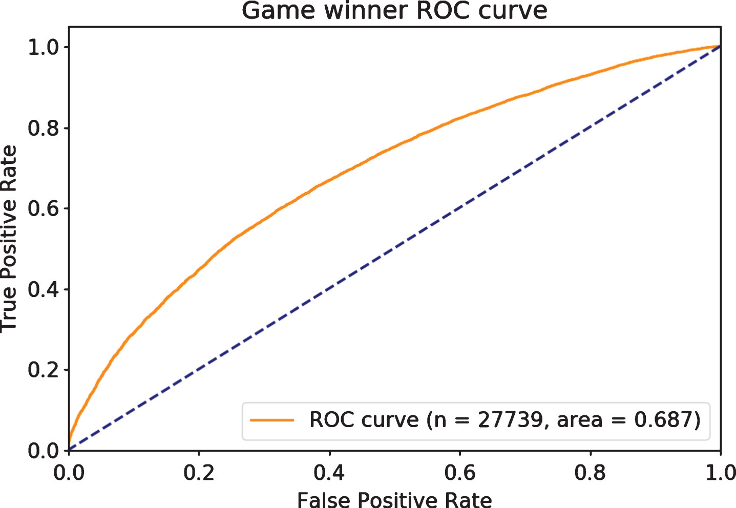
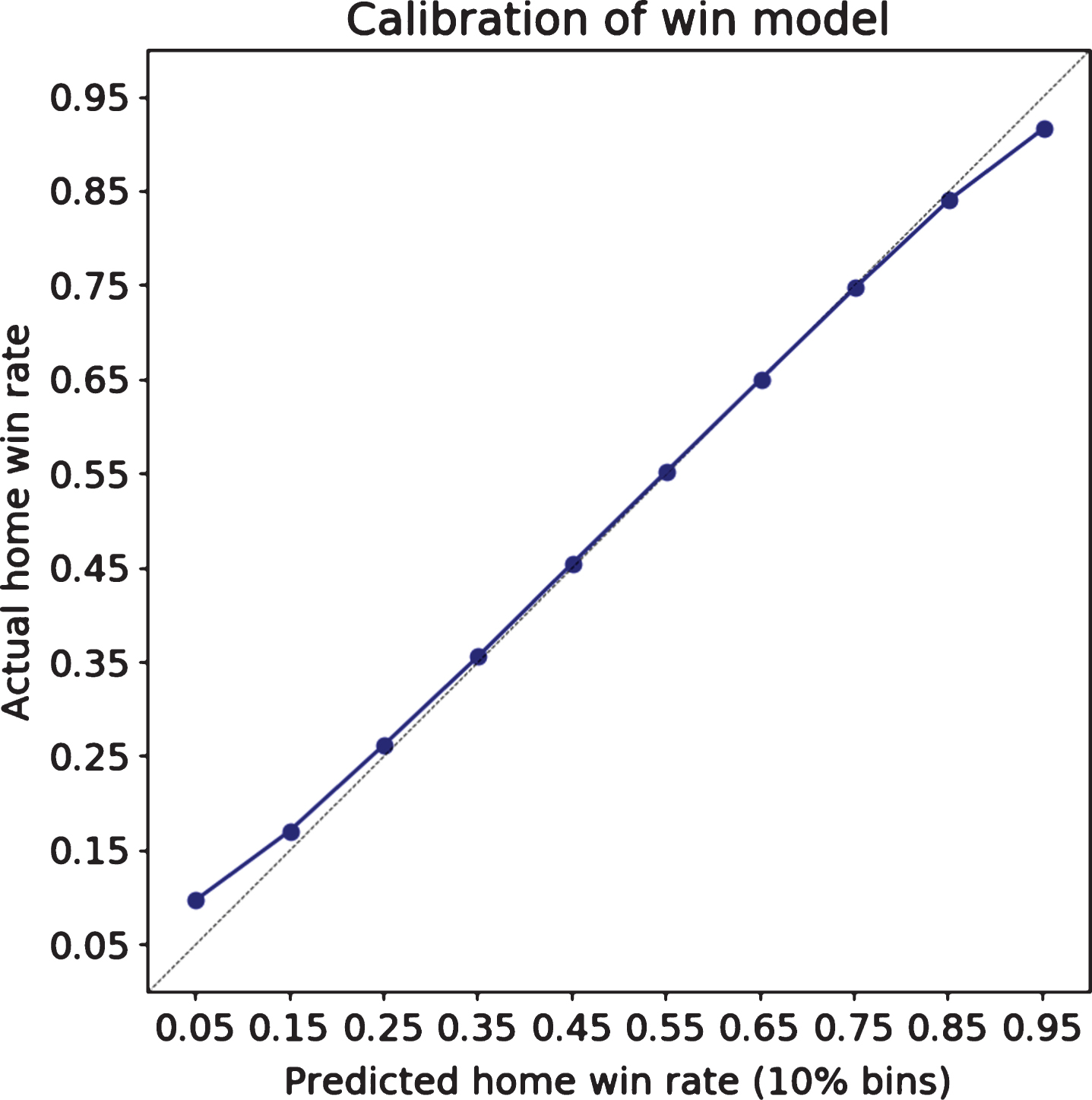
Fig.4
The probability of winning a given game is well-calibrated.
Now that we have reasonable individual game probabilities we can perform Monte Carlo simulations to evaluate the probability of each team making the playoffs for each season.
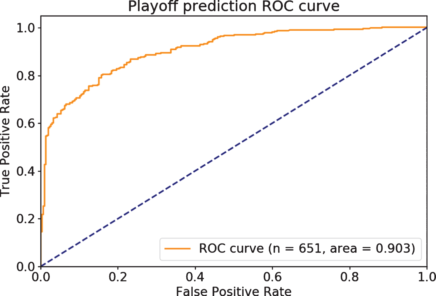
In the popular example of presidential election forecasting, we may never truly know if our models are calibrated correctly, since we only observe an election every four years. However, for basketball predictions we observe up to 30 observations each year. We have sample to statistically evaluate accuracy. Since in any specific season we only have up to 30 teams, and we have 22 years of attempted modeling, we end up with 651 playoff or non-playoff outcomes. For simplicity, rather than incorporate the actual playoff criteria, which has varied over time and includes a system of tiebreakers, we instead evaluate with an approximation. The approximation is whether the team ends up in the top eight teams in their conference by win-loss record. For most teams, this correctly identifies whether they made the playoffs of not. As long as we apply the same criteria to all of our playoff estimation procedures, our comparison is fair.
As shown in Fig. 5, the model very effectively ranks playoff probabilities. For the purpose of trying to predict, before the season even begins, which teams will make the playoffs, this system shows considerable precision.
Fig.5
The rank-ordering accuracy of playoff predictions.
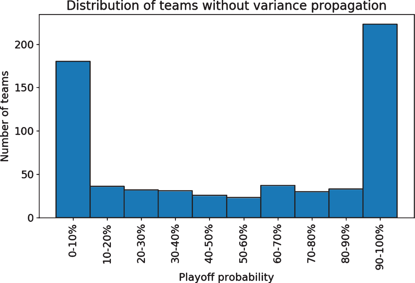
However, the playoff probabilities are very poorly calibrated, meaning that while the simulation ranks the teams correctly, the probabilities it generates are systematically inaccurate. This is despite the win model itself being well calibrated, as shown previously in Fig. 4. Across 10,000 simulations of each season, 47 teams were predicted to make the playoffs all 10,000 times, and 29 were predicted to miss it each of the 10,000 times, giving us Monte Carlo probabilities of 100% and 0%. That implies 76 of the 651 team seasons have certain outcomes, which is a clear canary in the coal mine. Given enough simulations the odds would not be exactly 100% or 0%, but to be so extreme is an indication of a severe problem. For context, in betting markets, ahead of the 2016-17 season no NBA team was given worse than 500-1 odds of winning the championship, and none had worse than 200-1 odds of winning their conference, let alone making the playoffs (Fawkes 2016). In our simulations without accounting for error correlation, 244 of the 651 teams are given odds of below 1% or above 99%. Fig. 6, with the distribution of playoff predictions, shows that only a minority of seasons are given unsure probabilities.
Fig.6
The model offers extremely low or high probabilities for many team seasons.
Our hypothesis is that unpredictable model errors will be correlated within a season, due to multi-game injuries, persistent player quality differences from the model, team streakiness, or other factors. This will lead the model without variance propagation to suffer from outcomes that are too similar across simulations, leading to overconfident playoff predictions. If this is true, then we should see error correlation from our game win model. If teams win (or lose) games they were not predicted to win (or lose), they are more likely to continue to win (or lose) more games than expected, for the reasons explained above. The nature of correlation could take many forms, but at its simplest it could be correlation between adjacent games. Across our out-of-sample game win predictions, home teams have an error correlation of 0.04, while away teams have an error correlation of 0.043, both of which are highly significant, given samples of 27,391 and 27,436, respectively. The counts of home and away pairs need not match, because our series are discontinuous at the end of seasons, and there need not be an equal amount of teams starting the season at home as on the road. Both correlations are positive, fitting our hypothesis. That these correlations are not larger speaks to the multitude of factors affecting games and the substantial randomness involved, two factors key to the entertainment value of sports.
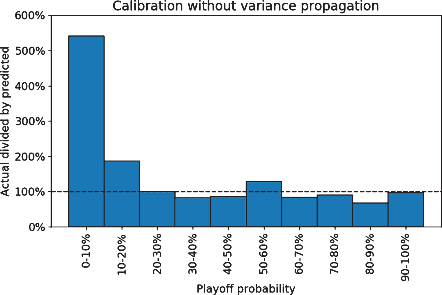
In Fig. 7 we can clearly see that our certainty is misguided. This chart groups team seasons by their playoff likelihoods, and then plots the number of teams making the playoffs versus the average predicted value. A well-calibrated model should be close to the 100% line, where the number of teams making the playoffs matches the amount we would expect based on the estimated probabilities. Instead, the low probability groups below 20% probabilities are all actually drastically underestimated by the Monte Carlo simulation, even by a factor of 5 in the below 10% group. In that group the model predicted under 2% of teams (3.7 of the 180) to make the playoffs, yet 20 (over 11%) did. Likewise, although it is not as obvious due to the scale, all of the high probability groups are overestimated. The Monte Carlo method leads us astray, overly certain that likely events will happen and that unlikely events will not happen.
Fig.7
Playoff probabilities are substantially inaccurate.
4.4Propagation of uncertainty
Depending on our modeling approach, correlation of errors in our first level models may result in unbiased estimates of win probabilities, but variance which is unaccounted for, resulting in incorrect playoff probabilities. If we can instead incorporate error correlation we can reach more plausible estimates.
When calculating probabilities, “stochastic simulation requires that an assumption be made about the distribution of the error terms and the coefficient estimates” (Fair 1986). Studies that do not directly incorporate error variance are implicitly choosing to assume no errors in the first level models, which can be particularly calamitous in cases of hierarchical models such as those demonstrated here. When we simulate we not only need to simulate using the probabilities given by the win model, but also across the values that we use in the player strength and minutes played models.
A simple method for the structure described above is to directly propagate the variance of the player quality and player minute predictions into our team quality metric, and thus into our win predictions. Instead of predicting each player’s quality and minutes and then holding those values constant in every simulation, we let those values vary. In each simulated season we generate stochastic error terms for each player for each of the BPM and MP models, and hold those constant across the season. The distributions “are almost always assumed to be normal, although in principle other assumptions can be made” (Ibid.). When we simulate the season again, we generate new error terms from the same distributions. These error terms are normally distributed, with means of 0 and standard deviations matching the prediction standard errors from the respective regressions.
This is not the only reasonable approach. Bayesian methods have long been used to explicitly structure and identify parameter uncertainty, since “at its core, Bayes’ theorem is a device for accounting for uncertainty” (Allenby et al. 2005). Box and Tiao (1965) directly frames this problem in a Bayesian setting, and Ansari et al. (2000) describes heterogeneity in Bayesian hierarchical models. Bayesian methods provide a strong theoretical base for how to reach posterior distributions for parameters given uncertainty and observed data. However, this paper retains the structure of multilevel regressions with playoff probabilities identified through Monte Carlo simulations. This is closer to the approach used by the sources we cited (Agami and Walsh 2013; Harris 2008; Restifo 2016; Boice 2015).
Our simulation gives us in-season error correlation that could mimic true error correlation. In Section 3.4 we described the situation of teams performing far worse than expectation due to long-lasting injuries that affect most or all of a season. If the forecaster makes predictions before the season, not knowing about upcoming injuries, they may have substantially correlated errors. The errors are not independent if they share a common cause. Simulating with stochastic error terms that are held constant across the season can generate these unlucky situations, which would otherwise never be simulated if each game was independent.
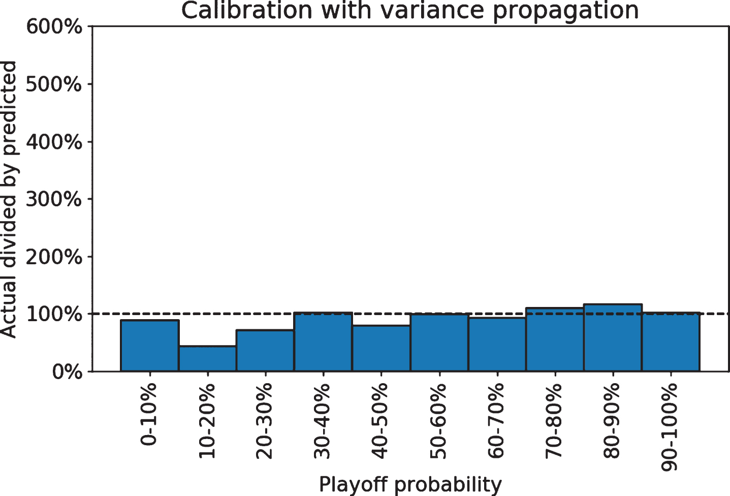
Applying this method we get distinctly less certain playoff predictions (Fig. 8) that are better calibrated and do not show consistent patterns of under- or over-estimation (Fig. 9).
Fig.8
The propagated model offers less certain probabilities.
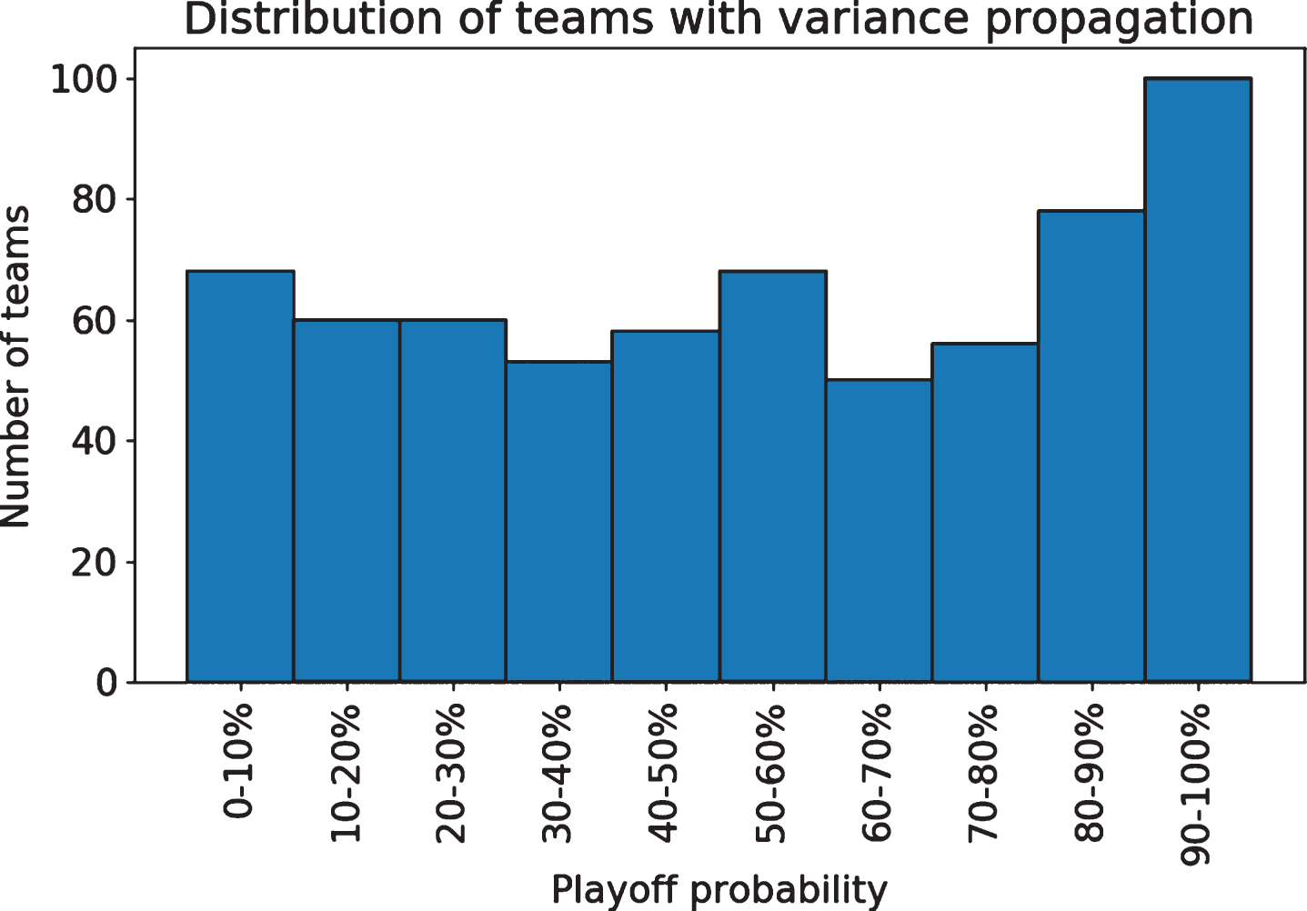
Fig.9
Playoff probabilities with propagation do not show systematic bias.
When evaluating multiple forecast models, the “standard procedure for ex post comparisons is to compute ex post forecasts over a common simulation period, calculate for each model and variable an error measure, and compare the values of the error measure across models” (Fair 1986). Mean squared error (MSE), also known as Brier score in forecast evaluation, is a common and simple metric for probability forecasts (Brier 1950). Overall, the simulation with variance propagation is similar by MSE to the unadjusted simulation, with a MSE of 0.1288 compared to 0.1323. However, the difference is most substantial in the extreme values. We can quantify the calibration differences by looking at the scale of errors in each simulation method, splitting into score ranges to show the dramatic error differences at low and high probabilities. For all of the lowest and highest probability ranges, the model with propagated variance improved on the naive model by having much lower mean squared error, as shown in Table 6.
Table 6
MSE by probability range and simulation method
| Probability | Variance propagated | Variance not propagated |
| (0-10%] | 0.04 | 0.10 |
| (10-20%] | 0.07 | 0.21 |
| (20-30%] | 0.15 | 0.19 |
| (30-40%] | 0.23 | 0.20 |
| (40-50%] | 0.23 | 0.24 |
| (50-60%] | 0.24 | 0.24 |
| (60-70%] | 0.23 | 0.25 |
| (70-80%] | 0.15 | 0.23 |
| (80-90%] | 0.03 | 0.31 |
| (90-100%] | 0.03 | 0.04 |
While we can compare the model against external predictions, we are limited by data availability for other models. Many create predictions before a particular season and do not repeat the process the next year, giving us only one year of out-of-time predictions. We can compare against those published at FiveThirtyEight, where predictions are stored from before and during the 2015-16 and 2016-17 season (Boice et al. 2015; Boice et al. 2016). Two years of data gives us only 60 binary playoff outcomes, with 32 teams making the playoffs, so suitable caution should be taken with deriving any conclusions. However this comparison will still provide a general indication of how confident and accurate the models are. Here we compare against the actual playoff outcomes instead of an approximation, since FiveThirtyEight publishes them as such.
The authors of the FiveThirtyEight model are aware of the error correlation problem, and took steps to ensure some correlation in their season samples by having their team strength metric increase or decrease with each simulated win or loss (Boice 2015). This creates momentum in team strength over a season, which could approximate some of the team quality changes that occur over time.
Even with this correlation strategy, the FiveThirtyEight model offers more certain predictions than our propagated model, with an average absolute deviation from 50% of 28% (i.e. the typical team has 78% or 22% playoff likelihoods) compared to the 26% of our model. The FiveThirtyEight model is not more confident of playoff or non-playoff status for every team, but it is for the majority of them (34 of 60). We can reasonably expect that other models that do not use any variance propagation will be more confident. Team-by-team results are shown in Tables 7 and 8.
Table 7
2015-16 playoff outcomes and probabilities (rounded)
| Team | Playoffs | Wins | FiveThirtyEight | Our Model |
| GSW | 1 | 73 | 98% | 99% |
| SAS | 1 | 67 | 97% | 90% |
| CLE | 1 | 57 | 99% | 94% |
| TOR | 1 | 56 | 78% | 91% |
| OKC | 1 | 55 | 97% | 84% |
| LAC | 1 | 53 | 95% | 90% |
| ATL | 1 | 48 | 85% | 90% |
| BOS | 1 | 48 | 90% | 80% |
| CHO | 1 | 48 | 60% | 58% |
| MIA | 1 | 48 | 48% | 59% |
| IND | 1 | 45 | 50% | 55% |
| DET | 1 | 44 | 45% | 45% |
| POR | 1 | 44 | 23% | 74% |
| DAL | 1 | 42 | 29% | 49% |
| MEM | 1 | 42 | 81% | 69% |
| HOU | 1 | 41 | 88% | 78% |
| CHI | 0 | 42 | 88% | 70% |
| WAS | 0 | 41 | 66% | 52% |
| UTA | 0 | 40 | 65% | 55% |
| ORL | 0 | 35 | 43% | 18% |
| DEN | 0 | 33 | 5% | 7% |
| MIL | 0 | 33 | 34% | 50% |
| SAC | 0 | 33 | 28% | 18% |
| NYK | 0 | 32 | 6% | 3% |
| NOP | 0 | 30 | 62% | 42% |
| MIN | 0 | 29 | 2% | 2% |
| PHO | 0 | 23 | 30% | 26% |
| BRK | 0 | 21 | 3% | 13% |
| LAL | 0 | 17 | 1% | 5% |
| PHI | 0 | 10 | 3% | 9% |
Table 8
2016-17 playoff outcomes and probabilities (rounded)
| Team | Playoffs | Wins | FiveThirtyEight | Our Model |
| GSW | 1 | 67 | 99% | 100% |
| SAS | 1 | 61 | 87% | 99% |
| HOU | 1 | 55 | 68% | 80% |
| BOS | 1 | 53 | 86% | 93% |
| CLE | 1 | 51 | 98% | 98% |
| LAC | 1 | 51 | 78% | 78% |
| TOR | 1 | 51 | 94% | 92% |
| UTA | 1 | 51 | 87% | 79% |
| WAS | 1 | 49 | 52% | 47% |
| OKC | 1 | 47 | 83% | 90% |
| ATL | 1 | 43 | 49% | 82% |
| MEM | 1 | 43 | 21% | 46% |
| IND | 1 | 42 | 46% | 52% |
| MIL | 1 | 42 | 25% | 34% |
| CHI | 1 | 41 | 80% | 53% |
| POR | 1 | 41 | 72% | 52% |
| MIA | 0 | 41 | 28% | 43% |
| DEN | 0 | 40 | 45% | 36% |
| DET | 0 | 37 | 57% | 46% |
| CHO | 0 | 36 | 79% | 58% |
| NOP | 0 | 34 | 21% | 19% |
| DAL | 0 | 33 | 31% | 41% |
| SAC | 0 | 32 | 20% | 28% |
| MIN | 0 | 31 | 72% | 30% |
| NYK | 0 | 31 | 39% | 43% |
| ORL | 0 | 29 | 49% | 34% |
| PHI | 0 | 28 | 15% | 3% |
| LAL | 0 | 26 | 3% | 1% |
| PHO | 0 | 24 | 12% | 8% |
| BRK | 0 | 20 | 3% | 7% |
Note that our model did not predict the 2016-17 Golden State Warriors would make the playoffs in literally 100% of simulations as the rounded table value would indicate, but rather 99.9% of simulations.
The FiveThirtyEight model had a mean squared error of 5.11% and a mean absolute deviation of 30.4%, compared to 4.25% and 25.7% for our model.
Among the predictions that did not succeed, FiveThirtyEight had the 2015-16 Bulls at 88% playoff odds and the Portland Trailblazers at 23%, and the 2016-17 Charlotte Hornets at 79% and the Memphis Grizzlies at 21%. Those Trailblazers and Grizzlies ultimately made the playoffs, while the Bull and Hornets did not. Our model has these teams at 70%, 74%, 58%, and 46%, respectively. While our model likewise classified incorrectly (or unluckily) in three of those cases, it did so to a lesser extent. Our model’s worst outcomes were those Bulls, and the 2016-17 Milwaukee Bucks at 34% —another case where the FiveThirtyEight model was incorrectly more confident, predicting only a 25% playoff chance.
Two seasons is very little to draw conclusions from, and these results are driven by only a handful of unexpected outcomes. Nevertheless, it should give some comfort in the plausibility of the model presented here.
5Conclusion
Playoff predictions in sports are commonly based on Monte Carlo simulations of underlying statistical models, and quite often these are subject to systematic bias. As described in this paper, Monte Carlo simulation unbiasedly estimates team win probabilities based on underlying models. However, playoff probabilities can be biased when the Monte Carlo procedure is applied without accounting for error correlation. These errors exist because the unpredictable variations in player performance and player health are correlated over time and are not, instead, i.i.d. across games within a season. This paper describes the problem in detail and demonstrates it through a plausible empirical model that accurately predicts game outcomes. If we fail to account for error correlation, we may predict extremely high or low playoff probabilities, which are demonstrably mis-calibrated when evaluated against realized outcomes. We can solve our calibration problem with passthrough variance, through which our powerful model will yield playoff probabilities that are not overconfident.
Acknowledgments
I thank Steve Scott, Lawrence Wang, Nelson Bradley, and Ken Tam for thoughtful reviews of drafts, as well as both Frank Meng and Peter Tanner for critical discussions. The data used in this paper was obtained from www.basketball-reference.com.
References
1 | Agami G., & Walsh S., (2013) , FanGraphs playoff odds. http://www.fangraphs.com/coolstandings.aspx?type=4 |
2 | Allenby G.M. , Rossi P.E. , & McCulloch R.E. (2005) , Hierarchical Bayes Models: A Practitioners Guide. https://papers.ssrn.com/sol3/papers.cfm?abstract_id=655541 |
3 | Ángel Gómez M. , Lorenzo A. , Sampaio J. , Ibáñez S.J. , & Ortega E. (2008) , Game-related statistics that discriminated winning and losing teams from the spanish mens professional basketball teams, Collegium Antropologicuml 32: (2). |
4 | Ansari A. , Jedidi K. , & Jagpal S., (2000) , A hierarchical bayesian methodology for treating heterogeneity in structural equation models, Marketing Science 19: , 328–347. |
5 | Association for Professional Basketball Research, 2016, 2016-17 Team Win Projection Contest / Discussion. http://apbr.org/metrics/viewtopic.php?f=2&t=9188 |
6 | Barrow D. , Drayer I. , Elliot P. , Gaut G. , & Osting B., (2013) , Ranking rankings: An empirical comparison of the predictive power of sports ranking methods, Journal of Quantitative Analysis in Sports 9: (2). |
7 | Berri D.J. , (1999) , Who is ‘most valuable’? Measuring the player’s production of wins in the National Basketball Association, Managerial and Decision Economics 20: (8). |
8 | Boice J. , (2015) , How our 2015-16 NBA predictions work. https://fivethirtyeight.com/features/how-our-2015-16-nba-predictions-work/ |
9 | Boice J. , Fischer-Baum R. , & Silver N., (2015) , 2015-16 NBA Predictions (Forecast from Oct 27). https://projects.fivethirtyeight.com/2016-nba-picks/ |
10 | Boice J. , Fischer-Baum R. , & Silver N., (2016) , 2016-17 NBA Predictions (Forecast from Oct 24). https://projects.fivethirtyeight.com/2017-nba-predictions/ |
11 | Box G.E.P. , & Tiao G.C., (1965) , A bayesian approach to the importance of assumptions applied to the comparison of variances, Biometrika 51: (1-2), 153–167. |
12 | Brier G.W. , (1950) , Verification of forecasts expressed in terms of probability, Monthly Weather Review 78: (1-3). |
13 | Chen J. , Tan X. , & Zhang R., (2008) , Inference for normal mixtures in mean and variance, Statistica Sinica 18: (2), 443–465. |
14 | Choudhury T. , (2010) , Learning with Incomplete Data. http://cs. dartmouth.edu/~cs104/CS104 11.04.22.pdf |
15 | Diebold F.X. , & Mariano R.S. (2002) , Comparing Predictive Accuracy, Journal of Business & Economic Statistics 20: (1), 134–144. |
16 | Do C.B. , & Batzoglou S., (2008) , What is the expectation maximization algorithm? Nature Biotechnology 26: (8), 897–899. |
17 | Dunlop D.D. , (1994) , Regression for longitudinal data: A bridge from least squares regression, The American Statistician 48: (4), 299–303. |
18 | Fair R.C. , (1986) , Evaluating the predictive accuracy of models, Handbook of Econometrics 3: , 1979–1995. |
19 | Fawkes B. , (2016) , Full list of 2017 NBA title odds. |
20 | Feller W. , (1945) , On the normal approximation to the binomial distribution, The Annals of Mathematical Statistics 16: (4), 319–329. |
21 | Gelman A. , (2016) , Explanations for that shocking 2%shift. http://andrewgelman.com/2016/11/09/explanations-shocking-2-shift/ |
22 | Harris M., (2008) , DVOA playoff odds report. http://www.footballoutsiders.com/stats/playoffodds |
23 | Loeffelholz B. , Bednar E. , & Bauer K.W., (2009) , Predicting NBA games using neural networks, Journal of Quantitative Analysis in Sports 5: (1). |
24 | Lynch M. , (2015) , SRS Calculation Details. |
25 | Manner H. , (2016) , Modeling and forecasting the outcomes of NBA basketball games, Journal of Quantitative Analysis in Sports 12: (1). |
26 | Metropolis N. , & Ulam S.M., (1949) , The monte carlo method, Journal of the American Statistical Association 44: (247), 335–341. |
27 | Myers D., (n.d.). About Box Plus/Minus (BPM). http://www.basketball-reference.com/about/bpm.html |
28 | Page G.L. , Fellingham G.W. , & Reese C.S. , (2007) , Using box-scores to determine a position’s contribution to winning basketball games, Journal of Quantitative Analysis in Sports 3: (4). |
29 | Restifo N. , (2016) , Hopefully possible win projections 2016-2017. http://nyloncalculus.com/2016/10/03/hopefully-possible-win-projections-2016-2017/ |
30 | Rey-Bellet L. , (2010) , Lecture 17: The Law of Large Numbers and the Monte-Carlo method. http://people.math.umass.edu/~lr7q/ps_files/teaching/math456/lecture17.pdf |
31 | Ruiz F.J.R. , & Perez-Cruz F., (2015) , A generative model for predicting outcomes in college basketball, Journal of Quantitative Analysis in Sports 11: (1). |
32 | Štrumbelj E. , & Vrača P., (2012) , Simulating a basketball match with a homogeneous Markov model and forecasting the outcome, International Journal of Forecasting 28: (2). |
33 | Vaz de Melo P.O.S. , Almeida V.A.F. , Loureiro A.A.F. , & Faloutsos C., (2012) , Forecasting in the NBA and Other Team Sports: Network Effects in Action, ACM Transactions on Knowledge Discovery from Data 6: (3). |
34 | West K.D. , (1996) , Asymptotic inference about predictive ability, Econometrica 64: (5), 1067–1084. |


