
Prediction of pitch type and location in baseball using ensemble model of deep neural networks
Abstract
In the past decade, many data mining researches have been conducted on the sports field. In particular, baseball has become an important subject of data mining due to the wide availability of massive data from games. Many researchers have conducted their studies to predict pitch types, i.e., fastball, cutter, sinker, slider, curveball, changeup, knuckleball, or part of them. In this research, we also develop a system that makes predictions related to pitches in baseball. The major difference between our research and the previous researches is that our system is to predict pitch types and pitch locations at the same time. Pitch location is the place where the pitched ball arrives among the imaginary grids drawn in front of the catcher. Another difference is the number of classes to predict. In the previous researches for predicting pitch types, the number of classes to predict was 2∼7. However, in our research, since we also predict pitch locations, the number of classes to predict is 34. We build our prediction system using ensemble model of deep neural networks. We describe in detail the process of building our prediction system while avoiding overfitting. In addition, the performances of our prediction system in various game situations, such as loss/draw/win, count and baserunners situation, are presented.
1Introduction
In sports, vast amounts of data are generated and collected by season, by game, by team, and by player. The vast amounts of data recorded in this way have been a heavy information overload for owners or managers who have to decide on game strategies and player scouts. It is true that in the past, these decisions have only relied on empirical judgments of some experts including owners, managers or coaches. However, the task of finding meaningful patterns from the vast amounts of data is almost impossible only with the empirical judgment of human experts. Therefore, various data mining techniques are actively being used to make reasonable decisions in the sports field. Needless to say, data mining cannot be a substitute for human experts. By presenting the results of analysis on the vast amounts of data, it helps the human experts to make more creative decisions.
Data mining is a process for exploring and analyzing large amounts of data to discover meaningful patterns and rules (Linoff and Berry, 2011). It has been applied in various fields such as business, science, engineering, healthcare, medicine, biology, genetics, pharmaceuticals and telecommunication. However, data mining is relatively a new technique in the sports field (Schumaker et al., 2010). Using modern information technology, massive data can be collected and analyzed in sports. The importance of data mining is already known by ‘Moneyball’, which was written by Michael Lewis (2003) and made into a movie in 2011. In this book, Billy Beane, an American baseball team manager at Oakland Athletics, shows how a team can be transformed into a strong team by evaluating players in a statistically based way under poor financial conditions. In these days, sports teams are interested in the field of data mining in order to evaluate their competitors and establish new strategies to enhance their competitiveness. The ‘Sports Analytics Conference’ has been held at MIT in USA since 2006 (MIT Sloan, 2022).
In this research, we develop a system that makes predictions related to pitches in professional baseball games. Unlike the previous researches for predicting pitch types only, we also predict pitch locations in addition to pitch types. After building our prediction system, we analyze how its performance changes in various game situations, such as loss/draw/win, count and baserunners situation. This paper is composed as follows. In Section 2, we describe previous researches on pitch type prediction in baseball. Section 3 deals with the collection and preparation of the data used in this research. Section 4 describes in detail how we built our prediction system. Section 5 evaluates the performance of our prediction system. Section 6 concludes this research.
2Pitch type prediction in baseball
Ganeshapillai and Guttag (2012) employed support vector machines (SVM) to predict six types of pitches, i.e., fastball, changeup, slider, curve, forkball and cut fastball. They used Major League Baseball (MLB) data of 359 pitchers who threw at least 300 pitches in both 2008 and 2009 seasons. The data was collected from PITCHf/x, a system developed by Sportvision that tracks the speeds and trajectories of pitched balls (Fast, 2010). The SVM models were trained using the data from 2008 season and tested on the data from 2009 season. However, those six types of pitches were not predicted at the same time by using one multiclass SVM. They built a total of six different SVM models, one for each type. In other words, they predicted fastball or not, changeup or not, slider or not, and so on by using six binary prediction models. The average accuracy of the six models was 65.8%, and the average accuracy of naïve prediction was 61.8%. Naïve prediction means that we simply predict that all predictions are the class that occupies the largest proportion of the data. A baseline for the usefulness of the model is whether it can do better than naïve prediction.
Hamilton et al. (2014) used SVM and k-nearest neighbors (k-NN) to predict only two types of pitches, i.e., fastball or nonfastball. They built their models using the data of 236 pitchers who threw at least 750 pitches in both 2008 and 2009 MLB seasons. Detailed results of eight pitchers were presented. For these eight pitchers, the average number of records collected per pitcher was 2,875. On average, SVM and k-NN showed similar accuracies, 79.8% and 80.9%, respectively. The average accuracy of naïve prediction was 66.0%. In addition, they demonstrated how their model’s accuracy changed in different count situations. The accuracy was higher in batter-favored counts such as 3-0 (3 balls and 0 strikes) and 2-0, and was lower in pitcher-favored counts such as 1-2 and 0-2.
Bock (2015) used the data from three MLB seasons, 2011∼2013. By excluding pitchers having thrown less than 1,000 pitches during the three seasons, he used the data of 402 pitchers to build his model. He first extracted the four pitch types each pitcher threw most frequently. For example, Justin Verlander’s most frequent pitches, in order of frequency, were fastball, changeup, curve and slider. Then he developed four separate binary classifiers using SVM with one-versus-rest strategy. The final decision on pitch type prediction was made according to the most positive magnitude of the decision function output from each classifier. He tested his model on 14 pitchers in the 2013 World Series game between the Boston Red Sox and the St. Louis Cardinals. The accuracy ranged from 50.2% to 69.8%. The average accuracy was 60.9%.
Sidle and Tran (2018) employed multiclass linear discriminant analysis (LDA), multiclass SVM and random forest to predict seven types of pitches, i.e., fastball, cutter, sinker, slider, curveball, changeup and knuckleball. They collected about 1,340,000 records of 287 pitchers who threw at least 500 pitches in both 2014 and 2015 MLB seasons. The average number of records collected per pitcher was 4,682. They used the data obtained from the games in the regular season of September and October 2016 as test data set. The average accuracy on the test data set was 59.1%, and the accuracy of naïve prediction was 52.1%.
In order to win a baseball game, the batter must hit the ball and go on base. The reason we want to predict the pitch in baseball is to give information to the batter so that he can hit the ball. In order for the batter to hit the ball, he needs to know where the ball is coming in, i.e., pitch location. Pitch location is the place where the pitched ball arrives among the imaginary grids drawn in front of the catcher. Prediction of pitch location has not been addressed in the previous researches. Therefore, pitch type predictions in the previous researches did not provide enough information that could be used practically in baseball games. The innovation of our research is to simultaneously predict pitch types and pitch locations.
3Data collection and preparation
A pitcher must throw the pitch that is the most appropriate for the current game situation. The game situations are whether his team is losing, drawing or winning, at which bases the runners are, what the current count is, and who the batter is, etc. However, the pitcher, the catcher and the manager may have different opinions on which pitch is the most appropriate. Therefore, the pitcher does not decide which pitch to throw alone, but by exchanging signs with the catcher, or at the direction of the manager. In other words, pitch decision is a group effort rather than an individual pitcher’s effort.
The prediction system in our research is not intended to predict the capabilities of individual pitchers, but rather to predict the most appropriate pitches determined by group efforts in various game situations. If we can predict the pitch type and pitch location using the data related to the current game situation, we can increase the probability that the batter hits the ball. This is the fundamental idea that motivated us to do this research.
Pitching data is not simply an accumulation of pitches thrown by individual pitchers, but rather an accumulation of pitches determined by group efforts. However, we have no way of knowing what kind of pitches were determined by group efforts until the pitcher actually throws the balls. Though pitch decision is a group effort, actual execution of throwing the ball is the sole responsibility of the pitcher. Therefore, the pitcher must successfully perform the determined pitches. In other words, once the pitch type and pitch location were determined, the pitcher must throw the ball of that type to that location. To do this, the pitcher should have the ability to throw the ball as he intended.
This kind of ability can be described in terms of ‘control’ and ‘command’ (Jenkins, 2011). ‘Control’ is the ability of a pitcher to locate his pitches. ‘Command’ is the ability of a pitcher to make the ball move the way it is intended to move. The pitcher has ‘control’ when the pitches he throws are staying in or out of the strike zone as he wants. In other words, ‘control’ refers to the ability of the pitcher to land the ball at the desired location. The pitcher’s ‘command’ means that his pitches are doing what he wants them to do. If his intention is to throw a curve ball, then the ball will curve, if his intention is to throw a slider ball, then the ball will slide. The target pitcher of our prediction system must have good ‘control’ and ‘command’ abilities. Therefore, we selected the pitcher ‘Y’ who was evaluated as having a high level of ‘control’ and ‘command’ abilities in the Korea Baseball Organization (KBO) league. We collected the data by analyzing the videos of 50 games where ‘Y’ played in 2015 and 2016 seasons, from the homepage of KBO. The pitch locations were collected from the strike zone displayed in the lower right corner of the game video screen.
One record of the collected data consists of 10 input attributes and 10 target attributes as shown in Table 1. For the progress input attribute, we collected the scores of two teams playing the baseball game. When building our models, we tried the score itself, score difference, and loss/draw/win. Among these, we decided to use the latter because the built models showed higher accuracies when using it. Ball and strike in target attribute were prefixed with ‘T’ to distinguish them from ball and strike in input attribute.
Table 1
Input and Target Attributes
| Category | Attribute | Values | |
| Input | Inning | InnNum | 1, 2, 3, 4, 5, 6, 7, 8, 9 |
| Progress | LDW | 1 = Loss; 2 = Draw; 3 = Win | |
| Runner | Base1 | 0, 1 | |
| Base2 | 0, 1 | ||
| Base3 | 0, 1 | ||
| Count | Ball | 0, 1, 2, 3 | |
| Strike | 0, 1, 2 | ||
| Out | 0, 1, 2 | ||
| Batter | Order | 1, 2, 3, 4, 5, 6, 7, 8, 9 | |
| LR | 1 = Left-handed; 2 = Right-handed | ||
| Target | Ball/Strike | T_Ball | 0, 1 |
| T_Strike | 0, 1 | ||
| Pitch Type | Fastball | 0, 1 | |
| Nonfastball | 0, 1 | ||
| Horizontal Location | Left | 0, 1 | |
| Center | 0, 1 | ||
| Right | 0, 1 | ||
| Vertical Location | Up | 0, 1 | |
| Middle | 0, 1 | ||
| Down | 0, 1 |
All target attributes in Table 1 are binary variables. The six attributes in ‘Horizontal Location’ and ‘Vertical Location’ categories, i.e., from ‘Left’ to ‘Down’, are represented as follows: We can draw nine gray imaginary grids in front of a catcher as shown in Fig. 1. We call it ‘Strike Zone.’ The white area outside of it is ‘Ball Zone.’ As seen in Fig. 1, this square is divided into ‘Left’, ‘Center’, ‘Right’ horizontally and ‘Up’, ‘Middle’, ‘Down’ vertically. Since we collected this data from the strike zone displayed in the game video screen, the left and right are positions seen from the pitcher’s point of view. The six attributes in ‘Horizontal Location’ and ‘Vertical Location’ categories along with the two attributes in ‘Ball/Strike’ category determine the pitch locations.
Fig. 1
Pitch Locations.
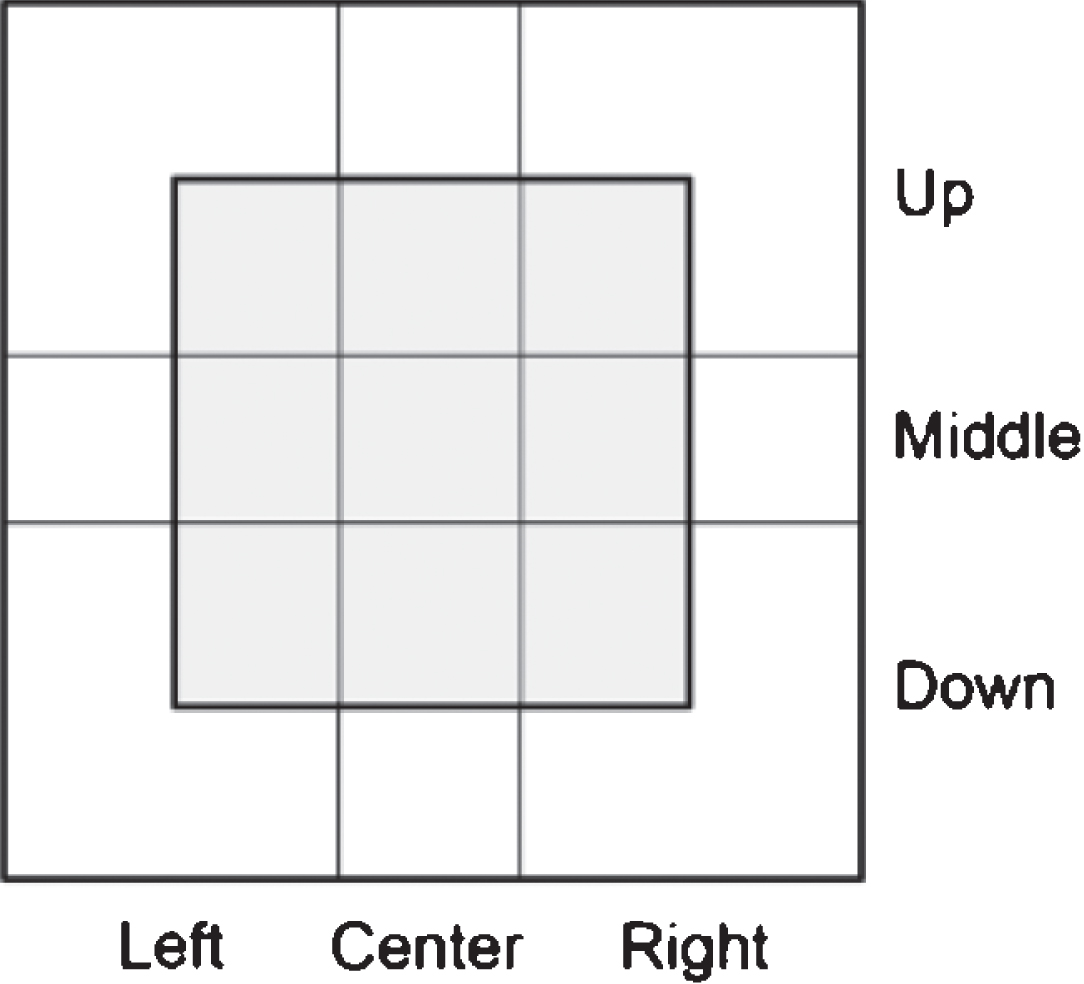
There are 17 pitch locations in Fig. 1 and a pitch type can be fastball or nonfastball. Therefore, the number of classes to predict is 34. A fourth ball that makes the batter walk to first base can be part of a strategy, but in our research we considered it as a pitcher’s mistake and excluded it from the collected data. In the case of foul balls, only the first foul ball was included in the data. After this preprocessing, the number of records in the model data set was 4,871.
Among 4,871 records, the five pitches with the largest frequencies are shown in Table 2 and illustrated in Fig. 2.
Table 2
Five Pitches with the Largest Frequencies
| Target Attributes | Frequency | |||||||||
| T_Ball | T_Strike | Fastball | Nonfastball | Left | Center | Right | Up | Middle | Down | |
| 1 | 0 | 0 | 1 | 1 | 0 | 0 | 0 | 0 | 1 | 401 (8.2%) |
| 0 | 1 | 1 | 0 | 1 | 0 | 0 | 0 | 0 | 1 | 374 (7.7%) |
| 0 | 1 | 0 | 1 | 1 | 0 | 0 | 0 | 0 | 1 | 302 (6.2%) |
| 0 | 1 | 1 | 0 | 0 | 0 | 1 | 0 | 0 | 1 | 263 (5.4%) |
| 0 | 1 | 0 | 1 | 0 | 0 | 1 | 0 | 0 | 1 | 235 (4.8%) |
Fig. 2
Locations of the Five Pitches with the Largest Frequencies.
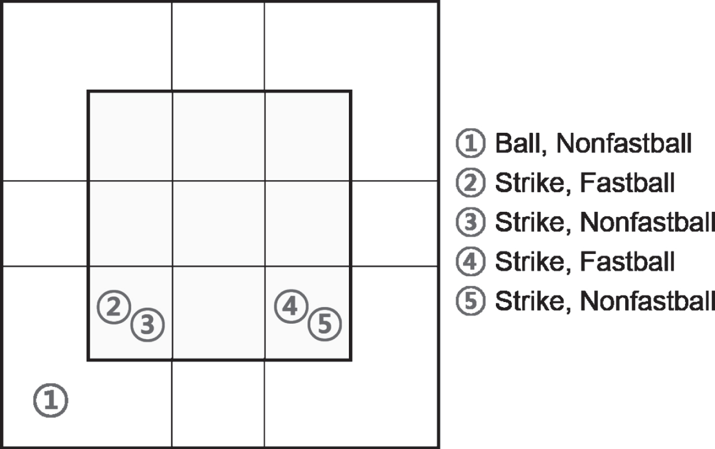
Verducci (2017) divided MLB pitchers into two categories, i.e., pitchers who love low strikes and pitchers who hate low strikes, and surveyed the batting average against (BAA) of 10 pitchers in each category. BAA is a statistic that measures a pitcher’s ability to prevent hits during official at bats, the lower the better. The BAA of the former category was 0.133∼0.25, with an average of 0.213, and the BAA of the latter category was 0.374∼0.404, with an average of 0.387. This result indicates that low pitches are difficult for batter to hit. Low pitches require a higher level of ‘control’ and ‘command’ abilities than high pitches, and this is a common opinion among baseball experts. As seen in Fig. 2, the five pitches with the largest frequencies are located in low zone. It indicates that the pitcher ‘Y’ we selected has a high level of ‘control’ and ‘command’ abilities.
4Model building process
4.1Detection and elimination of overfitting
When building a model, it is important to detect and eliminate overfitting. If the model complexity is excessive, then overfitting occurs, i.e., the model memorizes training data set instead of recognizing more general patterns (Hawkins, 2004). Overfitting must be eliminated in order to build the right model. Therefore, if overfitting is detected during model building, it should be eliminated by reducing the model complexity. The data set used for overfitting detection is validation data set. The occurrence of overfitting is illustrated in Fig. 3.
Fig. 3
Overfitting Occurred in Model M.
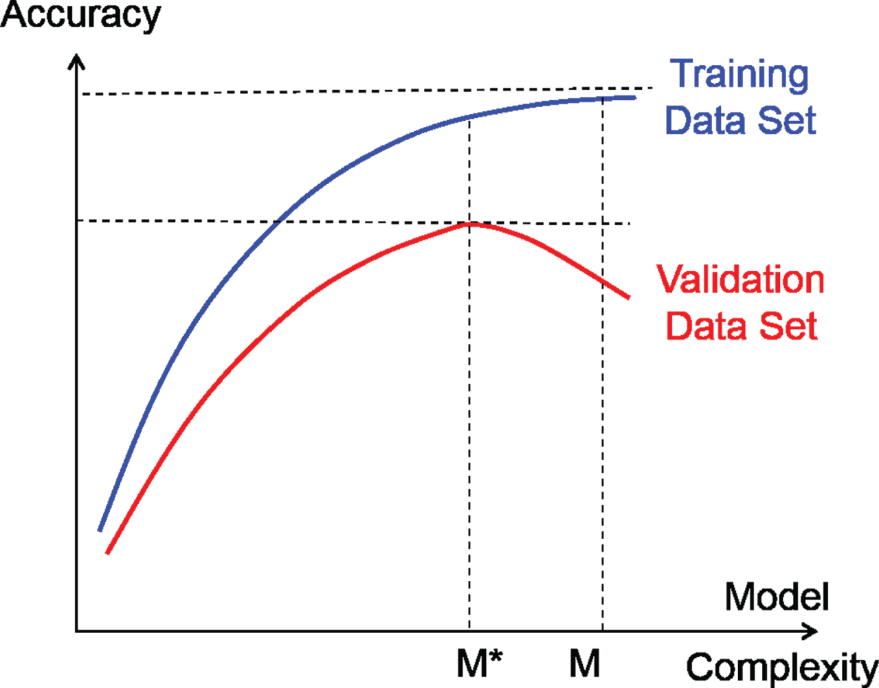
Let A(m:train) and A(m:valid) be the accuracy of model m on training data set and validation data set, respectively. Model M overfits training data set if there exists another model M* that shows lower accuracy on training data set, i.e., A(M*:train) < A(M:train), but shows higher or equal accuracy on validation data set, i.e., A(M*:valid)≥A(M:valid). As seen in Fig. 3, overfitting occurred in model M. Therefore, we should stop increasing the model complexity and select model M* as the final model.
4.2Deep neural network
Neural networks, also called artificial neural networks (ANNs), are based on the research of nerve cells and human brains. They consist of connections between nodes, also called processing elements, which mimic neurons, the basic units of the human brain. Each node receives multiple inputs and produces a single output. Generally, the output value of the preceding node is used as the input value of the subsequent node. ANN is a parallel distributed processing system, so it has a great advantage that several nodes operate and learn simultaneously. However, there is a limitation that overfitting can easily occur if the number of connections increases, and interpretation of results is difficult (Linoff and Berry, 2011).
Deep neural networks (DNNs) are basically neural networks with more than 2 hidden layers. DNN is one of the deep learning techniques together with convolutional neural network and recurrent neural network. ANN with 1 or 2 hidden layers is trained relatively well using a gradient-based learning algorithm such as backpropagation algorithm. However, if the number of hidden layers exceeds 2, it is not properly trained with the backpropagation algorithm. This is the vanishing gradient problem (Hochreiter, 1991). DNN has been developed by overcoming this vanishing gradient problem (Vanishing gradient problem, 2017). When building DNNs in this research, we used ReLU (Nair and Hinton, 2010) and logistic function for the activation functions of hidden layer and output layer, respectively. Initial weights for connections were set using Xavier initialization (Glorot and Bengio, 2010).
4.3Ensemble models of deep neural networks
An ensemble model is a model that builds multiple individual models and then combines the results from them to obtain one final result (Linoff and Berry, 2011). The individual models that make up the ensemble model are called base models. Previous research in which an ensemble model was used in sports analytics can be found in win-loss prediction. Saricaoğlu et al. (2020) built an ensemble model to predict home-team-win, away-team-win or draw of football matches in Turkish Super League. They used seven modeling techniques, such as LDA, quadratic discriminant analysis, k-NN, logistic regression, decision tree, bagging, SVM, and built 10 base models by varying the parameter values of some modeling techniques. The most predicted result by these 10 base models became the final result of the ensemble model. For example, if there were 4 home-team-wins, 3 away-team-wins, and 3 draws, then home-team-win became the final result. They collected a total of 936 records from five seasons and divided it into 749 (80%) and 187 (20%) for training and test data set. The accuracy of their ensemble model on the test data set was 62.0%. The accuracy of naïve prediction was 46.6%, the proportion of the most frequent case, i.e., home-team-win.
In this section, we describe how we built ensemble models of DNNs, i.e., E-DNN models. We built three E-DNN models as we improved their performances, and we called them E1-DNN model, E2-ENN model and E3-DNN model. We built our models using repeated random sub-sampling validation method, also known as Monte Carlo cross-validation method. Therefore, we prepared 10 different data sets, i.e., 10 splits, by stratified sampling of 60%, 20% and 20% for training, validation and test data set, respectively, from our model data set for 10 times. Among the 10 splits, we used the first split to determine the structure of model. We thoroughly checked to detect and eliminate overfitting while building our models.
4.3.1E1-DNN model
As seen in Table 1, our target consists of 10 attributes in four categories. For E1-DNN model, we built four DNNs, i.e., BS DNN, FNF DNN, LCR DNN and UMD DNN, for each of the four categories, as shown in Table 3.
Table 3
Four DNNs in E1-DNN Model
| Name | BS DNN | FNF DNN | LCR DNN | UMD DNN |
| Input | 10 Attributes in Table 1 | |||
| Output | T_Ball T_Strike | Fastball Nonfastball | Left Center Right | Up Middle Down |
Each base model, i.e., individual DNN, was built by varying the number of hidden layers and checking the occurrence of overfitting. Table 4∼7 show the accuracies of individual DNNs on training and validation data set as we increased the number of hidden layers. Because the connection weights can be set differently depending on the initial values and therefore the accuracy can vary, we created three models for each structure and thus we obtained three accuracies for each structure. Therefore, the accuracies presented in Table 4∼7 are the average values of these three accuracies.
Table 4
Structure Determination of BS DNN
| Number of Hidden Layers | Number of Nodes | Accuracy % | |||
| Input | Hidden | Output | Training | Validation | |
| 3 | 10 | 20-30-12 | 2 | 88.7 | 79.1 |
| 4 | 10 | 20-30-20-10 | 2 | 89.9 | 78.9 |
| 5 | 10 | 20-30-20-15-8 | 2 | 90.5 | 79.5 |
| 6 | 10 | 15-20-30-20-15-8 | 2 | 90.5 | 79.2 |
| 7 | 10 | 15-20-30-30-20-15-8 | 2 | 90.8 | 80.2 |
| 8 | 10 | 15-20-25-30-30-20-15-8 | 2 | 91.0 | 79.0 |
| 9 | 10 | 15-20-25-30-35-30-25-15-8 | 2 | 90.6 | 78.7 |
Table 5
Structure Determination of FNF DNN
| Number of Hidden Layers | Number of Nodes | Accuracy % | |||
| Input | Hidden | Output | Training | Validation | |
| 3 | 10 | 20-30-12 | 2 | 86.4 | 73.2 |
| 4 | 10 | 20-30-20-10 | 2 | 88.6 | 75.2 |
| 5 | 10 | 20-30-20-15-8 | 2 | 89.4 | 76.3 |
| 6 | 10 | 15-20-30-20-15-8 | 2 | 89.6 | 77.2 |
| 7 | 10 | 15-20-30-30-20-15-8 | 2 | 90.1 | 76.4 |
| 8 | 10 | 15-20-25-30-30-20-15-8 | 2 | 90.3 | 76.0 |
| 9 | 10 | 15-20-25-30-35-30-25-15-8 | 2 | 90.4 | 76.2 |
Table 6
Structure Determination of LCR DNN
| Number of Hidden Layers | Number of Nodes | Accuracy % | |||
| Input | Hidden | Output | Training | Validation | |
| 3 | 10 | 20-30-15 | 3 | 80.8 | 69.0 |
| 4 | 10 | 20-30-20-10 | 3 | 85.2 | 70.6 |
| 5 | 10 | 20-30-20-15-9 | 3 | 85.5 | 70.4 |
| 6 | 10 | 15-20-30-20-15-9 | 3 | 86.2 | 70.5 |
| 7 | 10 | 15-20-30-30-20-15-9 | 3 | 87.3 | 71.5 |
| 8 | 10 | 15-20-25-30-30-20-15-9 | 3 | 87.5 | 71.6 |
| 9 | 10 | 15-20-25-30-35-30-25-15-9 | 3 | 87.4 | 71.8 |
| 10 | 10 | 15-20-25-30-35-35-30-25-15-9 | 3 | 87.6 | 72.7 |
| 11 | 10 | 15-20-25-30-35-40-35-30-25-15-9 | 3 | 87.8 | 71.6 |
Table 7
Structure Determination of UMD DNN
| Number of Hidden Layers | Number of Nodes | Accuracy % | |||
| Input | Hidden | Output | Training | Validation | |
| 3 | 10 | 20-30-15 | 3 | 71.3 | 62.3 |
| 4 | 10 | 20-20-20-10 | 3 | 81.3 | 66.8 |
| 5 | 10 | 20-30-20-15-9 | 3 | 85.2 | 69.9 |
| 6 | 10 | 15-20-30-20-15-9 | 3 | 86.1 | 69.8 |
| 7 | 10 | 15-20-30-30-20-15-9 | 3 | 86.5 | 69.6 |
| 8 | 10 | 15-20-25-30-30-20-15-9 | 3 | 87.0 | 70.2 |
| 9 | 10 | 15-20-25-30-35-30-25-15-9 | 3 | 86.9 | 70.9 |
| 10 | 10 | 15-20-25-30-35-35-30-25-15-9 | 3 | 86.9 | 71.4 |
| 11 | 10 | 15-20-25-30-35-40-35-30-25-15-9 | 3 | 87.3 | 72.1 |
| 12 | 10 | 15-20-25-30-35-40-40-35-30-25-15-9 | 3 | 87.5 | 71.5 |
As seen in Table 4, the accuracy on validation data set reached the highest value 80.2% when the number of hidden layers was 7, which is written in bold type. After that, it showed the sign of overfitting. Therefore, the structure of BS DNN was determined as having 7 hidden layers. In the same manner, we determined the structures of the other three individual DNNs.
As seen in Tables 4∼7, the numbers of hidden layers in BS DNN, FNF DNN, LCR DNN and UMD DNN were determined as 7, 6, 10 and 11, respectively. Figure 4 shows the structure of E1-DNN model.
Fig. 4
Structure of E1-DNN Model.
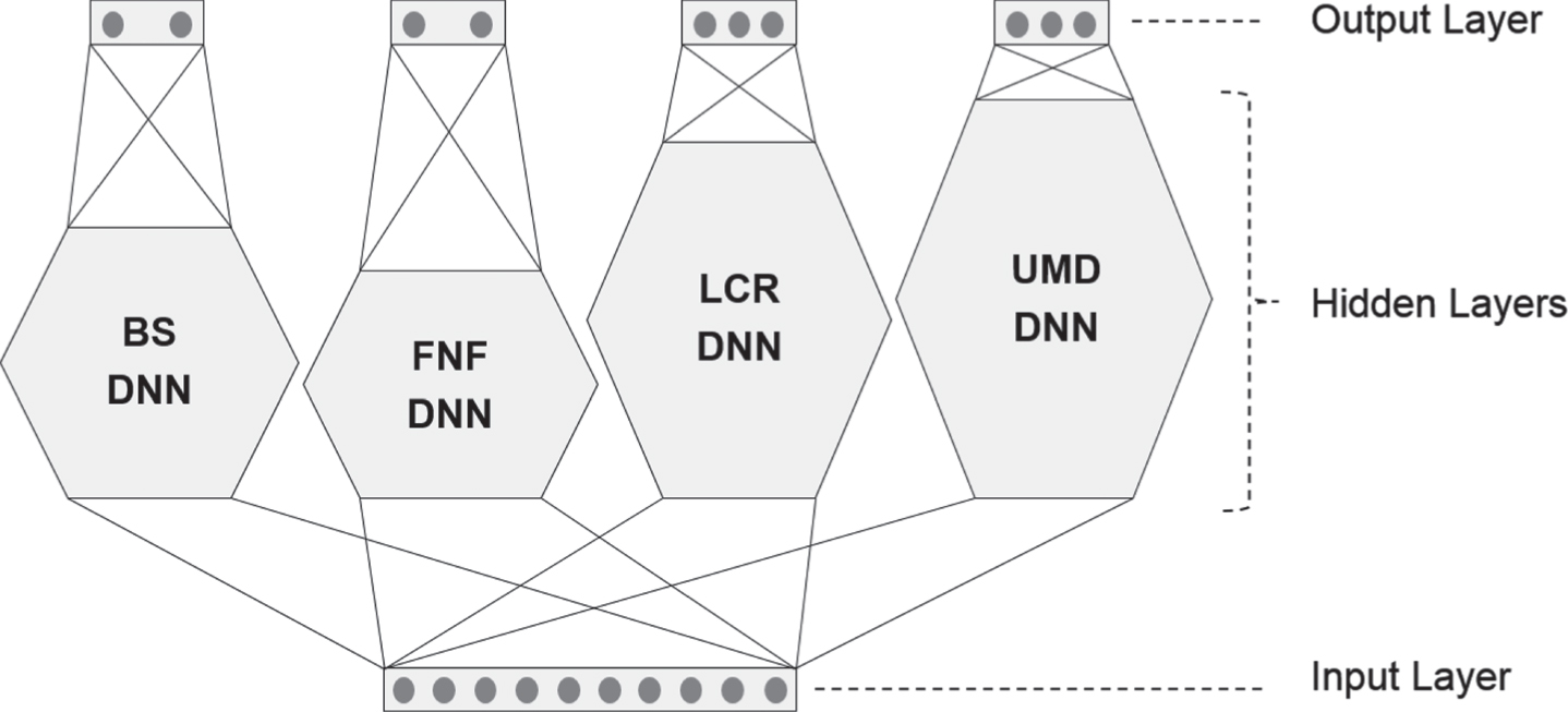
In most ensemble models, the final result is obtained by voting, i.e., the class predicted by most base models wins, for classification problem, and by averaging the results of base models for regression problem. However, the final result of our ensemble model is obtained in a different way. As seen in Fig. 4, when a record is input, the four individual DNNs share the same input values, but produce four separate sets of output values. The final result of E1-DNN is obtained by concatenating these four separate sets. If this final result matches the target values of that record, then E1-DNN succeeded in prediction.
The learning process of E1-DNN model stopped when the accuracy of E1-DNN model on validation data set did not increase during the preset number of iterations. Table 8 shows the accuracies of individual DNNs and E1-DNN model on training and validation data sets. The accuracies presented in Table 8 are the average values of the 10 accuracies obtained from 10 splits.
Table 8
Accuracies of E1-DNN Model
| BS DNN | FNF DNN | LCR DNN | UMD DNN | E1-DNN Model | ||||||
| Train | Valid | Train | Valid | Train | Valid | Train | Valid | Train | Valid | |
| Accuracy | 90.7 | 77.1 | 89.7 | 74.6 | 87.1 | 70.3 | 87.1 | 68.4 | 74.5 | 47.8 |
As seen in Table 8, the accuracy of E1-DNN model is too low compared to the accuracies of individual DNNs. High accuracies of individual DNNs do not guarantee a high accuracy of E-DNN model. The final result of E-DNN for a record is correct only when all 4 individual DNNs’ predictions for that record are correct.
4.3.2E2-DNN model
In Table 8, we can see that the accuracies of LCR DNN and UMD DNN are low compared to those of BS DNN and FNF DNN. The number of output nodes of LCR DNN and UMD DNN is 3, whereas that of BS DNN and FNF DNN is 2. Since the low accuracy might be due to the larger number of output nodes, we reduced the number of output nodes of LCR DNN and UMD DNN to 2 using the encoding method shown in Fig. 5.
Fig. 5
Encoding of Locations.
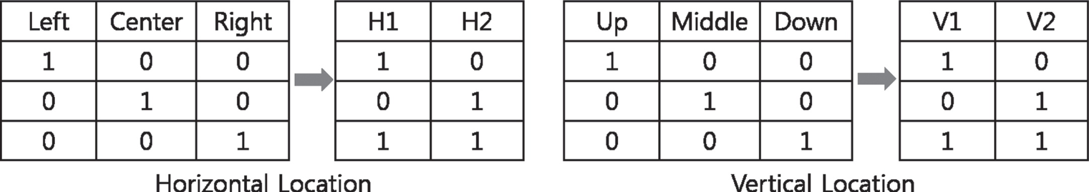
With this modification, we built E2-DNN model where LCR DNN was changed to HL DNN and UMD DNN was changed to VL DNN. Figure 6 shows the structure of E2-DNN model.
Fig. 6
Structure of E2-DNN Model.
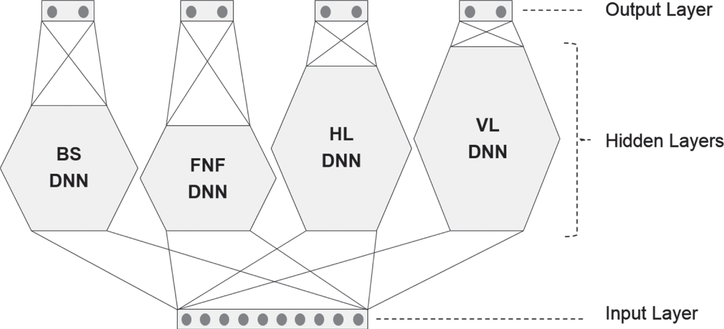
Table 9 shows the accuracies of individual DNNs and E2-DNN model on training and validation data sets. The accuracies presented in Table 9 are the average values of the 10 accuracies obtained from 10 splits.
Table 9
Accuracies of E2-DNN Model
| BS DNN | FNF DNN | HL DNN | VL DNN | E2-DNN Model | ||||||
| Train | Valid | Train | Valid | Train | Valid | Train | Valid | Train | Valid | |
| Accuracy | 93.3 | 80.5 | 92.3 | 77.9 | 89.8 | 72.0 | 89.9 | 70.9 | 82.9 | 56.9 |
As seen in Table 9, the accuracies of HL DNN and VL DNN increased compared to those of LCR DNN and UMD DNN shown in Table 8. Not only that, the accuracies of BS DNN, FNF DNN and E2-DNN model also increased. We can see that the accuracies of BS DNN and FNF DNN in Table 9 are different from those of BS DNN and FNF DNN in Table 8. This is not unusual. That is because, as we mentioned earlier, the learning process of E2-DNN model stopped when the accuracy of E2-DNN model on validation data set did not increase during the preset number of iterations.
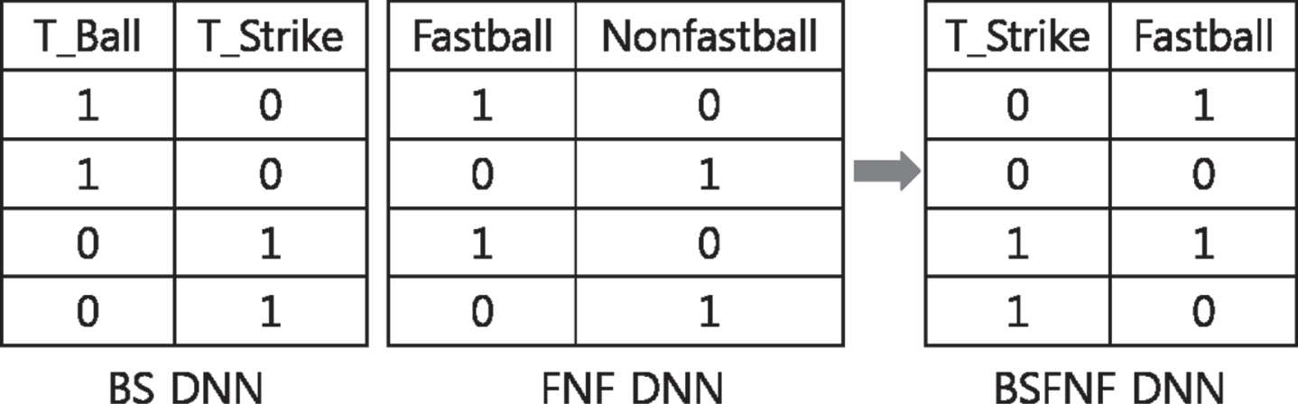
4.3.3E3-DNN model
Here we made one more modification to increase the accuracy of our ensemble model. Both BS DNN and FNF DNN had 2 output nodes each of which has a binary value. Therefore, two DNNs were not needed. One DNN, which we called BSFNF DNN, with 2 binary output nodes was sufficient as shown in Fig. 7.
Fig. 7
Merger of BS DNN and FNF DNN.
Since the number of individual DNNs and the number of their output nodes changed, we determined the structures of individual DNNs again. The structure determination process is the same as we described in Section 4.3.1. Table 10∼12 show the accuracies of individual DNNs on training and validation data set as we increased the number of hidden layers. As mentioned earlier, we created three models for each structure and thus we obtained three accuracies for each structure. Therefore, the accuracies presented in Table 10∼12 are the average values of these three accuracies.
Table 10
Structure Determination of BSFNF DNN
| Number of Hidden Layers | Number of Nodes | Accuracy % | |||
| Input | Hidden | Output | Training | Validation | |
| 8 | 10 | 15-20-25-30-30-20-15-8 | 2 | 87.3 | 65.3 |
| 9 | 10 | 15-20-25-30-35-30-25-15-8 | 2 | 88.8 | 65.6 |
| 10 | 10 | 15-20-25-30-35-35-30-25-15-8 | 2 | 89.0 | 64.2 |
| 11 | 10 | 15-20-25-30-35-40-35-30-25-15-8 | 2 | 88.9 | 63.8 |
Table 11
Structure Determination of HL DNN
| Number of Hidden Layers | Number of Nodes | Accuracy % | |||
| Input | Hidden | Output | Training | Validation | |
| 6 | 10 | 15-20-30-20-15-8 | 2 | 88.4 | 70.6 |
| 7 | 10 | 15-20-30-30-20-15-8 | 2 | 88.2 | 74.1 |
| 8 | 10 | 15-20-25-30-30-20-15-8 | 2 | 88.6 | 70.8 |
| 9 | 10 | 15-20-25-30-35-30-25-15-8 | 2 | 88.8 | 71.8 |
Table 12
Structure Determination of VL DNN
| Number of Hidden Layers | Number of Nodes | Accuracy % | |||
| Input | Hidden | Output | Training | Validation | |
| 11 | 10 | 15-20-25-30-35-40-35-30-25-15-8 | 2 | 90.2 | 71.1 |
| 12 | 10 | 15-20-25-30-35-40-40-35-30-25-15-8 | 2 | 90.3 | 73.3 |
| 13 | 10 | 15-20-25-30-35-40-45-40-35-30-25-15-8 | 2 | 90.3 | 72.0 |
| 14 | 10 | 15-20-25-30-35-40-45-45-40-35-30-25-15-8 | 2 | 90.4 | 71.0 |
As seen in Tables 10∼12, the numbers of hidden layers in BSFNF DNN, HL DNN and VL DNN were determined as 9, 7 and 12, respectively. Figure 8 shows the structure of E3-DNN model.
Fig. 8
Structure of E3-DNN Model.
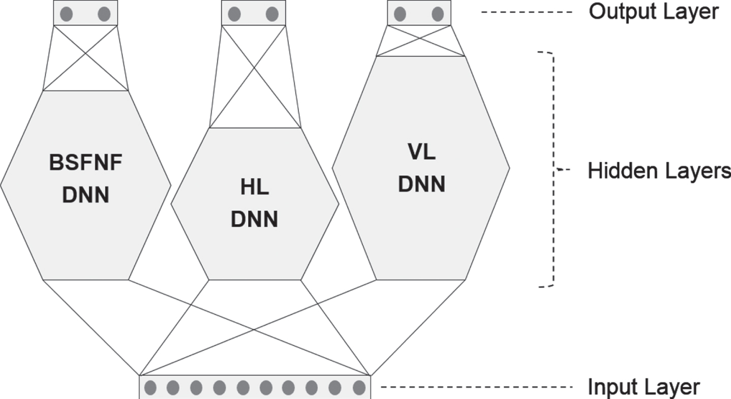
Table 13 shows the accuracies of individual DNNs and E3-DNN model on training and validation data sets. The accuracies presented in Table 13 are the average values of the 10 accuracies obtained from 10 splits.
Table 13
Accuracies of E3-DNN Model
| BSFNF DNN | HL DNN | VL DNN | E3-DNN Model | |||||
| Train | Valid | Train | Valid | Train | Valid | Train | Valid | |
| Accuracy | 88.5 | 65.9 | 89.3 | 71.5 | 90.1 | 70.5 | 85.7 | 61.1 |
As seen in Table 13, the accuracy of BSFNF DNN in E3-DNN model is lower than those of BS DNN and FNF DNN in E2-DNN model shown in Table 9. However, the accuracy of E3-DNN model is higher than that of E2-DNN model. The reason is that the number of cases in which all 3 individual DNNs’ predictions for a record were correct increased.
Among the three E-DNN models we built, E3-DNN model showed the highest accuracy on validation data set. Therefore, we selected E3-DNN model as our final model and named it ‘Ensemble of DNNs for Pitch Prediction’ or EP2 for short.
5Evaluation of EP2
In this section, we evaluate the performance of EP2 in detail. Table 14 shows the accuracies of EP2 on test data sets.
Table 14
Accuracies of EP2 on Test Data Sets
| Split # | EP2 |
| 1 | 64.4 |
| 2 | 63.1 |
| 3 | 62.9 |
| 4 | 61.6 |
| 5 | 62.9 |
| 6 | 62.8 |
| 7 | 62.7 |
| 8 | 60.2 |
| 9 | 61.2 |
| 10 | 62.6 |
| Average | 62.4 |
As seen in Table 14, the accuracy of EP2 on test data set is 62.4%. As shown in Table 2, the proportion of the pitch with the largest frequency is 8.2%, which is the accuracy of naïve prediction. Therefore, the accuracy increase of EP2 over naïve prediction is 54.2% point. Our data contains 4,871 pitches thrown to 1,276 batters. It means that the pitcher threw 3.8 balls per batter on average. Suppose the pitcher throws four balls to a batter. Then, as shown in (1), the probability that EP2 can predict at least one pitch correctly among these four balls, say P1 (4) , is 98.0%. This probability will increase as the number of pitches thrown increases.
(1)
Now we analyze the performance of EP2 in various game situations. As in the previous accuracy calculations, the accuracies presented in this section were also calculated using Monte Carlo cross-validation method, i.e., the average of 10 accuracies on test data set.
Figure 9 shows the accuracy by loss/draw/win situation of the pitcher’s team. The numerical value written at the bottom of each bar in the graph is the accuracy of naïve prediction. Accuracy is higher when the pitcher’s team is losing. It can be inferred that the pitcher pitches based on a predictable pattern when his team is losing.
Fig. 9
Accuracy by Loss/Draw/Win Situation.
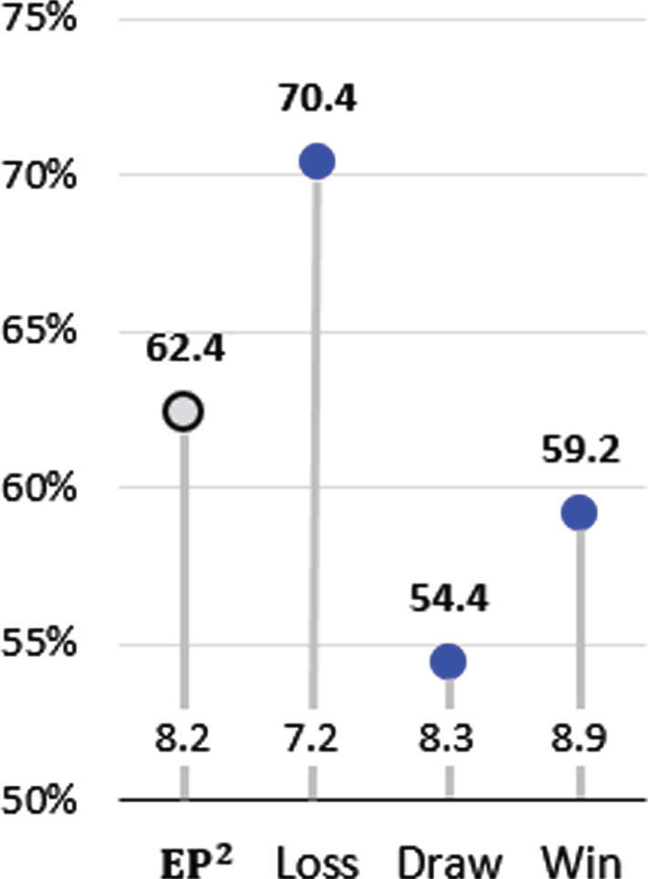
Figure 10 shows the accuracy by count situation. As described in Section 2, count 3-0 represents 3 balls and 0 strikes. Accuracy is significantly higher in batter-favored counts such as 3-0, 3-1 and 2-0, and is lower in pitcher-favored counts such as 2-2, 1-2 and 0–2. It can be inferred that the pitcher pitches based on a predictable pattern when the count is unfavorable to him. However, when the count is favorable to him, he is not burdened. He can afford to waste one or two pitches, so he can freely pitch balls that are difficult to predict.
Fig. 10
Accuracy by Count Situation.
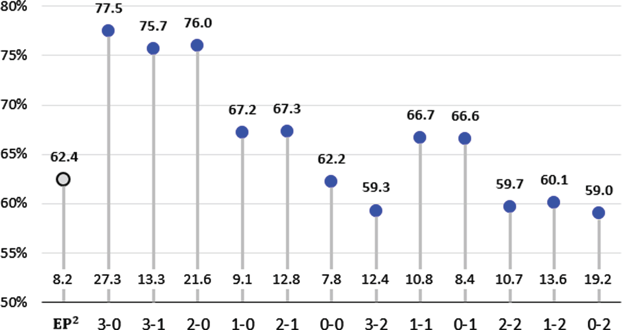
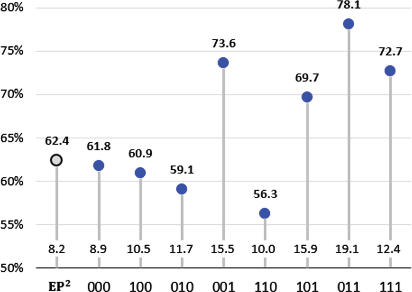
Figure 11 shows the accuracy by baserunners situation. Each of the three binary digits represents whether there is a runner at each base. For example, 000 represents there are no runners at bases, 110 represents there are runners at first and second bases, and 111 represents bases are full. Accuracy is significantly higher when there is a runner at third base, i.e., 001, 101, 011 and 111. A runner is said to be in scoring position when he is at second or third base because he can score on a single. A runner at third is more threatening because he can definitely score on a single or he can even score by stealing home plate. Similar to our previous analysis, it can be inferred that the pitcher pitches based on a predictable pattern when the baserunners situation is unfavorable to him.
Fig. 11
Accuracy by Baserunners Situation.
As we described, loss/draw/win, count and baserunners situations show a significant effect on accuracy. However, the other input attributes such as inning, batter lineup and batter handedness showed no effect on accuracy.
The result of the above three analyses shows that the pitcher pitches based on a predictable pattern when the game situation is unfavorable to him. As described in Section 2, we can find the similar result in Hamilton et al. (2014). They demonstrated how their model’s accuracy for predicting two pitch types varied by count situation. Therefore, we think that it may be possible to generalize the change in predictability according to the game situation.
6Conclusion
In this research, we developed a system to predict pitch types and pitch locations in baseball. Unlike the previous researches for predicting pitch types only, we also predicted pitch locations in addition to them. Therefore, the number of classes to predict was 34, which was larger than that in the previous researches. We built three ensemble models of deep neural networks and selected the one with the best accuracy, and named it EP2. The accuracy of naïve prediction was only 8.2%, but the accuracy of EP2 reached 62.4%.
We made interesting findings by analyzing the performance of EP2 in various game situations. The findings showed that the pitcher pitched based on a predictable pattern when the game situation was unfavorable to him. The accuracy of EP2 was higher when the pitcher’s team was losing or ball count was unfavorable to him or a runner was at third base, i.e., in scoring position. Therefore, it can be inferred that we can predict the pitch more accurately when the pitcher is in a difficult situation.
We developed one prediction system for a single pitcher using his data only. Despite the large number of classes to predict, we obtained a reasonably high level of accuracy. Therefore, we believe that it is better to build a pitch prediction system individually customized to each pitcher. However, since pitch selection is a group effort, pitches to be thrown in certain game situations can be very similar. In this respect, we think that our prediction system can be used for other pitchers as well. However, in this case, we have to take the risk of some reduction in accuracy. Although we described the system development process for a single pitcher, it can be applied to other pitchers as well to develop customized prediction systems suitable for them.
Our research has a limitation that the data size is small. While, in most previous researches, one prediction system was developed using data of several pitchers, our research was to develop a prediction system customized to a single pitcher. Therefore, we collected pitching data of only one pitcher, and the number of records used in our research was 4,871. It is small compared to that used in the previous researches where pitching data of several pitchers were collected. However, it is similar to the number of records collected per pitcher in the previous researches. Since there is no automatic pitch recording system like PITCHf/x in Korea, we collected the data while watching the recorded videos of baseball game. Therefore, vast amounts of data of several pitchers could not be collected. If we collect several pitchers’ data with an automatic pitch recording system, we can develop a pitch prediction system for each of them. Then we will be able to analyze the differences or similarities between the pitchers in various game situations. Since pitches are carried out consecutively, the location of the previous pitch or the game situation caused by the previous pitch, e.g., whether it was a hit or a home run, could affect the current pitch decision. Therefore, input attributes that can represent the pitch sequence and the resulting game situation can be added to the data used for building pitch prediction systems. This is left for further research.
Acknowledgment
I would like to thank the students in d2I (data to Intelligence), a data mining study group I supervise at Ajou University, for collecting the data for this research.
References
1 | Bock, J. R. , (2015) , Pitch Sequence Complexity and Long-Term Pitcher Performance, Sports, 3: (1), 40–55. |
2 | Fast, M. , (2010) , What the Heck is PITCHf/x, Hardball Times Baseball Annual, 6: , 153–158. |
3 | Ganeshapillai, G. and Guttag, J. , 2012, Predicting the Next Pitch, Proceedings of the MIT Sloan Sports Analytics Conference, Boston, MA, USA, March. |
4 | Glorot, X. and Bengio, Y. , 2010, Understanding the Difficulty of Training Deep Feedforward Neural Networks, Proceedings of the 13th International Conference on Artificial Intelligence and Statistics, 249–256. |
5 | Hamilton, M. , Hoang, P. , Layne, L. , Murray, J. , Padget, D. , Stafford, C. and Tran, H. , 2014, Applying Machine Learning Techniques to Baseball Pitch Prediction, Proceedings of the 3rd International Conference on Pattern Recognition Applications and Methods, 520–527. |
6 | Hawkins, D. M. , (2004) , The Problem of Overfitting, Journal of Chemical Information and Computer Science, 44: , 1–12. |
7 | Hochreiter, S. , 1991, Untersuchungen zu Dynamischen Neuronalen Netzen. Diploma Thesis, TU Munich. |
8 | Jenkins, C. S. , 2011, Control vs. Command, http://60ft6in.com/about/control-vs-command/ (Accessed: 14 March 2018). |
9 | Lewis, M. , (2003) , Moneyball: The Art ofWinning an Unfair Game, W. W. Norton & Company. |
10 | Linoff, G. and Berry, M. , (2011) , Data Mining Techniques: For Marketing, Sales, and CRM, 3rd ed., Wiley Pub. Inc., |
11 | MIT Sloan, Sports Analytics Conference, 2022, http://www.sloansportsconference.com/. |
12 | Nair, V. and Hinton, G. E. , 2010, Rectified Linear Units Improve Restricted Boltzmann Machines, Proceedings of the 27th International Conference on Machine Learning, 807–814. |
13 | Saricaoğlu, A. E. , Aksoy, A. and Kaya, T. , 2020, Prediction of Turkish Super League Match Results Using Supervised Machine Learning Techniques, in Intelligent and Fuzzy Techniques in Big Data Analytics and Decision Making, Kahraman, C., Cebi, S., Cevik Onar, S., Oztaysi, B., Tolga, A. and Sari, I. (Eds), Springer, Cham, Switzerland, 273–280. |
14 | Sidle, G. and Tran, H. , (2018) , Using Multi-Class Classification Methods to Predict Baseball Pitch Types, Journal of Sports Analytics, 4: (1), 85–93. |
15 | Schumaker, R. P. , Solieman, O. K. and Chen, H. , (2010) , Sports Data Mining, Springer. |
16 | Vanishing gradient problem, 2017, https://en.wikipedia.org/wiki/Vanishing_gradient_problem (Accessed: 10 June 2018). |
17 | Verducci, T. , 2017, Players who love—and hate—low strikes and could be impacted by potential rule change, https://www.si.com/mlb/2017/02/13/low-strikes-hitters-pitchers-top-10(Accessed: 20 May 2018). |


