
Modeling T20I cricket bowling effectiveness: A quantile regression approach with a Bayesian extension
Abstract
Bowling effectiveness is a key factor in winning cricket matches. The team captain should decide when to use the right bowler at the right moment so that the team can optimize the outcome of the game. In this study, we investigate the effectiveness of different types of bowlers at different stages of the game, based on the conceded percentage of runs from the innings total, for each over. Bowlers are generally categorized into three types: fast bowlers, medium-fast bowlers, and spinners. In this article, the authors divided the twenty over spell of a T20I match into four stages; namely, Stage 1: overs 1-6 (PowerPlay), Stage 2: overs 7-10, Stage 3: overs 11-15, and Stage 4: overs 16-20. To understand the broad spectrum of the behavior of game variables, a Quantile Regression methodology is used for statistical analysis. Following that, a Bayesian approach to Quantile Regression is undertaken, and it confirms the initial results.
1Introduction and motivation
Cricket is one of the most popular games in the world, especially in the commonwealth countries. It is similar to baseball in the sense that two teams of 11 players each compete. Each team takes its turn to bat and tries to score runs while also protecting the wickets. A coin toss outcome determines the first team batting, which takes place just prior to the first innings. The fielding team tries to dispatch each batsman, while simultaneously limiting the number of runs conceded. There are two main formats of limited overs cricket: One Day International (ODI) and T20I (Twenty20 International). Although new, the latter format is rapidly becoming popular among cricket fans due to its shorter match time (Manage and Scariano (2013)).
The first men’s T20I took place on February 17th, 2005 between teams from Australia and New Zealand (Ray (2019)). The International Cricket Council (ICC) introduced this new cricket format with the primary purpose to allure and captivate more fans to the sport. Our objective here is to investigate the bowling effectiveness of different types bowlers at different stages of the match.
For those new to the sport, a few terms and rules of cricket are first highlighted. Bowling is the action of propelling the ball toward the wicket which is defended by a batsman, also called a striker. A player who delivers a ball to a striker is called a bowler. A single act of bowling the ball toward a batsman is called a delivery. Bowlers bowl in sets of six deliveries, called overs. A bowler cannot bowl two or more overs consecutively. Fast-pace bowling and spin bowling are the two main types. A bowler must bounce the ball on the ground at most once before it reaches the batsman. A bowler can bowl a maximum of only one-fifth, or four (4), of the total of twenty (20) overs in the T20I format. Thus, a team needs at least five (5) bowlers to encompass twenty overs. The first six overs of an innings is described as the mandatory PowerPlay. There are certain field restrictions that the fielding team must follow during the PowerPlay. For example, only two fielders are allowed outside the 30-yard circle; and, beginning with the seventh over, no more than five fielders are allowed outside this circle. Additionally, a maximum of five fielders can be on the leg-side of the batsman at any given point in the innings.
As mentioned, there are primarily two types of bowling techniques in cricket: fast bowling (pace bowling/swing bowling) and spin bowling. Fast bowlers can be subcategorized into different types according to their preferred bowling speed (Table 1), and spin bowlers (spinners) can likewise be sub-categorized relative to the bowling styles adopted (Table 2). For simplicity throughout this study, all the spin bowling styles are identified as spinners, while fast or fast-medium bowlers are identified as fast bowlers. Finally, medium-fast and medium bowlers are identified as medium-fast bowlers.
Table 1
Classification of Fast and Medium Bowlers
| Type | km/h | mph |
| Fast | ≥ 141 | ≥ 88 |
| Fast-Medium | 130-141 | 81-88 |
| Medium-Fast | 120-129 | 75-80 |
| Medium | 100-119 | 62-74 |
Table 2
Bowling Styles
| Bowling Type | Bowling Style | Description |
| Fast | raf | Right-arm fast |
| laf | Left-arm fast | |
| rafm | Right-arm fast medium | |
| lafm | Left-arm fast medium | |
| Medium | ram | Right-arm medium |
| lam | Left-arm medium | |
| ramf | Right-arm medium fast | |
| lamf | Left-arm medium fast | |
| Spin | lb/leg | Legbreak |
| lbg/lg | Legbreak googly | |
| raob/rao | Right-arm offbreak | |
| ralb | Right-arm legbreak | |
| laob | Left-arm offbreak | |
| slao/laos | Slow left-arm orthodox/Left-arm orthodox spin | |
| slac | Slow left-arm chinaman | |
| lag | Left-arm googly |
A dismissal occurs when a batsman is called out, which is also known as taking, or losing, a wicket. Once a batsman is out, that batsman must discontinue batting and leave the field. Since strikers bat in pairs, when a batsman is called out, another batsman from the batting team comes to the field to complete the pair. "All out" is called when a bowling team dismisses the entire batting team by taking ten (10) wickets, assuming players from the batting team have not retired due to injury.
For modeling purposes, an innings in this study is divided into four stages. Stage 1 is comprised of the first six (6) overs. With fielding restrictions applied, batsmen try to take advantage of them to score as many runs as achievable, and as quickly as possible. On the other hand, bowlers try to take advantage of the PowerPlay by pressuring batsman to play risky shots. Overs seven (7) to ten (10) are identified as Stage 2, and this is usually the stage where spinners are introduced. During this stage, the batsmen pursue a strategy of accumulating runs to reach the planned total score, while concurrently protecting wickets vigorously. If the batting team has just a few dismissals in Stage 1, then Stage 2 is critical for the batting team to potentially adjust their innings strategy. Stage 3 consists of overs eleven (11) to fifteen (15). If Stage 2 has been satisfactorily accomplished, batsmen next try to accelerate the run-scoring rate while not relinquishing further wickets. Stage 4 comprises the final five (5) overs, and here batsmen try to score as many runs as possible with the goal of a higher total; or reaching a target set by the competing team in the event it is the first bowling team. Due to the shorter length of the twenty-over format, it is very common that the match usually protracts to Stage 4. In this instance, the batsmen are trying to score runs to surpass the score achieved by the first batting team or to score the highest possible total to set a competitive target for the opposing team. Regardless, the last few overs of the innings, Stage 4, cause excitement and anticipation intensifies significantly.
Several studies that address bowling performance, or runs conceded, can be found in the literature, including (Kimber (1993), Lemmer (2002), Van Staden (2009), and Akhtar, Scarf, and Rasool (2015)). These efforts have focused largely on the behavior of the mean, or average, of the runs conceded per over. Of course, the mean can reveal important aspects of a distribution in many cases. However, it is only one aspect of the distribution of a random variable that may be either quite compressed or exceedingly volatile across distinct subsets of its support, in such a manner that the average itself cannot reveal the more profound aspects of its distribution. Here, we use the percentage of runs conceded in each over to quantify bowling strength. Numerous factors such as pitch condition, wind speed, match importance, team performance on a given day, batting team’s ability to score runs all induce much variation in match outcome (Lohawala and Rahman (2018) and Fernando, Manage, and Scariano (2013)). Targeting the percentage of runs conceded (or scored) per over, rather than just the total number of runs conceded (or scored) per over should alleviate the effects of the conditions just mentioned and permit a clearer focus on true bowling effects. The bowling strategy of the second bowling team can greatly be affected by the target score set by the first batting team. Because of this, we only consider data from the first bowling team in our analysis.
Quantile regression is a statistical technique whose purpose is modeling the quantiles of a response variable. This methodology is a popular regression tool used by statisticians, and it is commonly applied in fields such as economics and epidemiology. The traditional Ordinary Least Squares (OLS) method is used to model the conditional mean of a response variable, but in some cases it has insurmountable shortcomings. For example, in some applications a one unit change in a predictor variable can, at differing quantiles of a response variable, be accompanied by differing parameter estimates, and OLS fails to model this scenario appropriately. Quantile regression works well when a response variable is continuous with no zeros or not too many repeated values (Benoit and Van den Poel (2017) and Lancaster and Jae Jun (2010)). In this study, quantile regression is used to model the response variable (percentage runs conceded per over) against different stages of the game and different bowling styles for T20I cricket matches. The main objective here is to analyze lower (or higher) runs conceding overs, which would, in turn, lead to lower (or higher) total final scores in a cricket match.
2Methodology
2.1Quantile regression
Quantile Regression (QR) was introduced as a robust alternative to OLS regression (Koenker and Bassett Jr. (1978)). However, the foundational aspects of quantile regression were introduced by Ruder Boscovich in the 18th century and more fully developed by Pierre-Simon Laplace and Francis Edgeworth during the 19th century (Leider (2012)). Although Quantile Regression methods require substantial computational effort, rapid technological developments in computational mathematics over the last three decades have now made this field of application feasible in real time.
Quantile Regression has several appealing advantages over the OLS method. In this technique, error terms do not necessarily adhere to the usual assumptions that they be independent and identically distributed (iid) normal variates. So, QR is generally more robust to the presence of outliers.
In a regression context, a median is usually defined as a solution to the problem of minimizing a sum of (symmetric) absolute residuals. A simple "tilting" results in a sum of (asymmetric) absolute residuals, which can be minimized to produce quantiles other than the median. This suggests solving
(1)
Fig. 1
Asymmetric Loss Function.
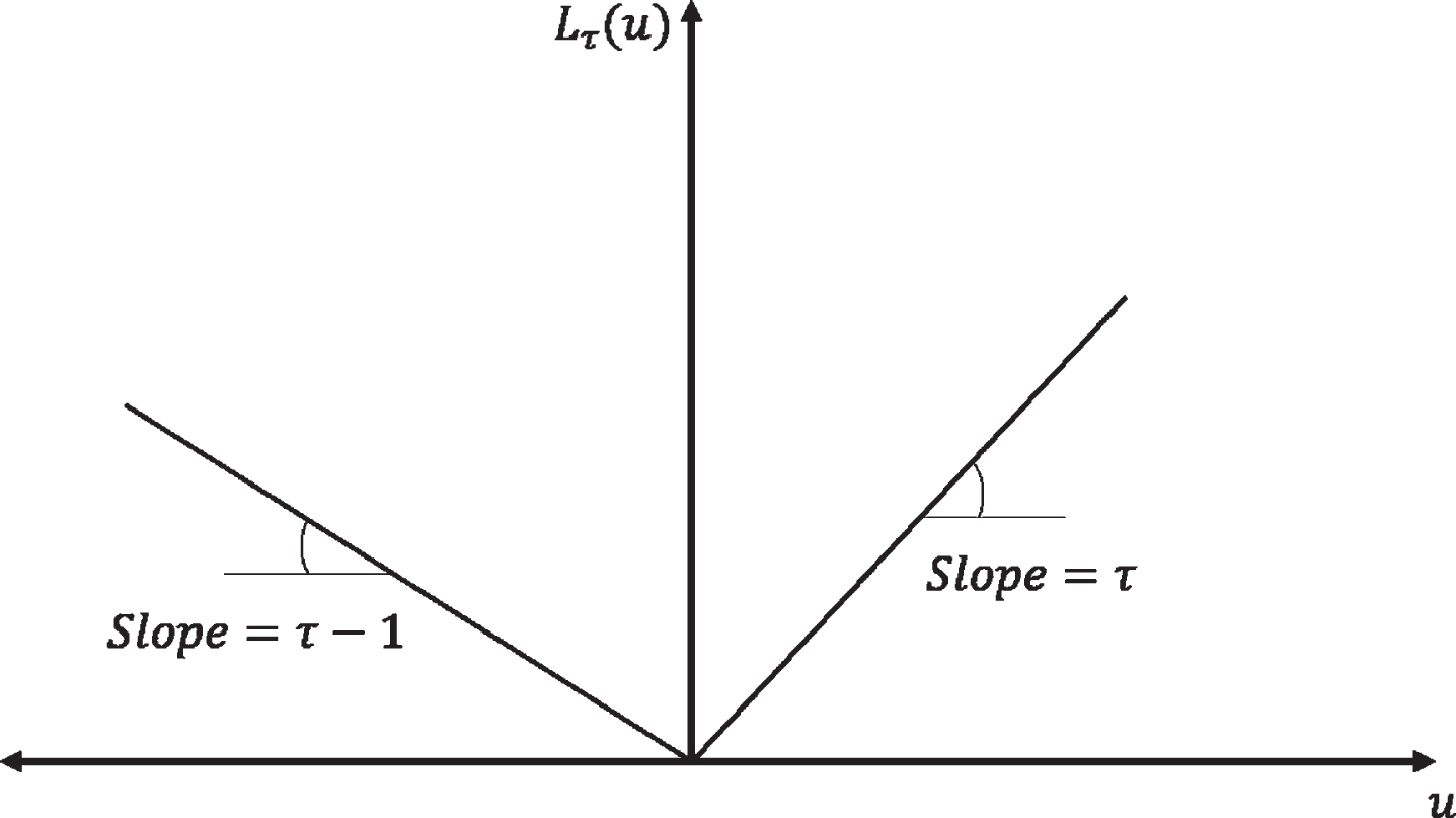
More specifically, Quantile Regression uses the asymmetric loss function:
(2)
To see that this loss function yields the desired sample quantiles, it is only necessary to compute the directional derivative, from the left and right, and with respect to ζ, of the objective function in Equation 1. In general, if F (x) is the cumulative distribution function and f (x) is the probability density function of a random variable X, then
(3)
This expectation is minimized when
In many practical applications, a cumulative density function is unknown to the investigator and must be estimated on the basis of data. Typically, the empirical cumulative distribution function is used for this purpose, as will be the case here as well.
To estimate the quantile function, consider
The Ordinary Least Squares method requires minimizing the error sum of squares, ei; that is,
For median regression, τ = 0.5 and
is to be minimized. Expanding this expression by substituting the regression model and labeling it as Q (βτ) produces
Note that whenever
The parameter estimates of the quantile regression model
3Descriptive data analysis
Data collected for this study comprised all T20I matches played up to May 5th 2019. It consists of matches played among the nine (9) ICC teams: Australia, Bangladesh, England, India, New Zealand, Pakistan, South Africa, Sri Lanka, and West Indies. Specifically, there are a total of 8,040 observations (overs), but matches with no results were omitted from this study. All data were collected from the official ESPN Cricinfo website (www.espncricinfo.com). However, due to technical difficulties, data with match IDs 41, 93, and 296 were inaccessible at the time of collection, so those observations were excluded.
For this study, innings were divided into four stages: Stage 1 (overs 1-6, Powerplay), Stage 2 (overs 7-10), Stage 3 (overs 11-15), and Stage 4 (overs 16-20). For simplicity, bowlers were grouped into three basic types: Fast, Medium and Spin. A detailed description of the bowling styles, abbreviations, and bowling types are summarized in Table 1 and Table 2. SAS 9.4 (www.sas.com) statistical software was used for all analyses undertaken in the study.
Of the 402 matches considered in this study, the first bowling teams lost 213 (52.99 %) matches and won 181 (45.02 %) matches. Eight matches (1.99 %) ended in a tie. The maximum number of runs conceded by the first bowling team was 263 while the minimum number of runs conceded by a team was 96 runs. On average, the first bowling team conceded 164.23 runs with a standard deviation of 29.81 runs. The Economy Rate, which is the number of runs conceded per over, is a key statistic used to measure the performance of a bowler. Having a low Economy Rate is regarded as being a key attribute for winning a match. The first bowling team won 85.71% of the matches it played when having an Economy Rate less than 6.0. On the other hand, the first bowling team won only 42.55% of the matches it played when the Economy Rate exceeded 6.0. Clearly, bowlers must concede as few runs as possible in order to increase the likelihood of winning a match.
Exploring the distribution of bowling styles across the various teams, how bowlers concede runs in general, and how bowlers concede runs at different stages of a match are quite interesting questions. Consideration of these bowler characteristics helps in gaining insight into how each team utilizes bowlers to maximize their chance of winning.
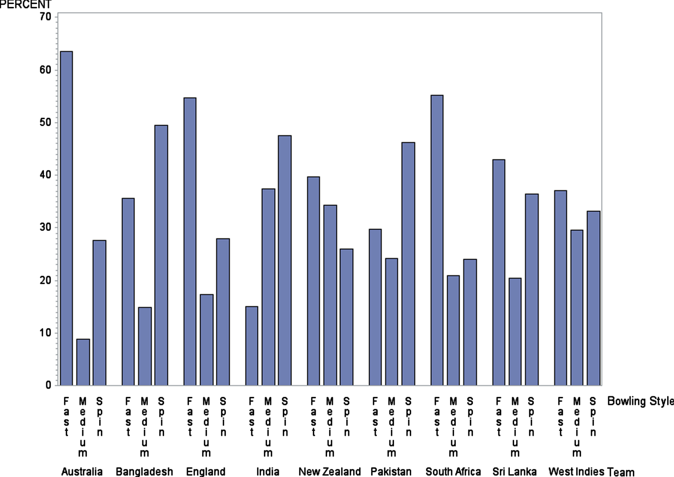
As seen in Table 3, for T20I cricket, in total, 42.57% of overs were bowled by fast bowlers, 34.81% of overs were bowled by spinners, and 22.61% of overs were bowled by the medium-fast bowlers. However, these percentages vary greatly among different teams. Figure 2 shows a clustered bar chart of the percentage of overs bowled by different types of bowlers, across each ICC team. Clearly, Australia, England, and South Africa prefer utilizing fast bowlers. Sri Lanka and West Indies seem to prefer using slightly more fast bowlers than spinners. In contrast, other Asian teams, such as Bangladesh, India, and Pakistan prefer to use more spinners than fast bowlers or medium-fast bowlers. Except for India and New Zealand, all the other teams utilize medium-fast bowlers less frequently. Evidently, New Zealand prefers using more fast bowlers and fewer spinners, while India prefers more spinners and fewer fast bowlers.
Table 3
Percentage of Overs Bowled by Different Types Bowlers
| Bowling Style | Percentage |
| Fast | 42.57% |
| Medium | 22.61% |
| Spin | 34.81% |
Fig. 2
Distribution of Bowling Types Across Different Teams.
The average percentage of runs conceded per over by different bowling styles is shown in Table 4. The highest average percentage of runs conceded per over is associated with medium-fast bowlers, and the spinners have conceded the fewest. The standard deviations of the runs conceded per over by fast bowlers and medium-fast bowlers are somewhat higher than for spinners. In terms of Economy Rate spinners performed well in the T20I format. Fast bowlers conceded fewer runs per over than medium-fast bowlers with a slightly higher standard deviation.
Table 4
Average Percentage of Runs per Over Conceded by Different Types of Bowlers
| Bowling Style | Mean | Standard Deviation |
| Fast | 5.17 | 2.74 |
| Medium | 5.20 | 2.68 |
| Spin | 4.66 | 2.54 |
The second column of Table 5 provides the overall average percentage of runs conceded per over in Stages one (1) through four (4). Fielding restrictions are applied during the PowerPlay (Stage 1), with the intent of providing advantage to the batting team for scoring many runs, while also keeping the game quite interesting for fans. However, on average, runs conceded per over during the PowerPlay are generally fewer than those in Stages three (3) and four (4). Stage two (2) typically produces the fewest average runs conceded per over when compared to all other stages. Usually, the highest average number of runs conceded per over occurs in Stage four (4), when no additional field restrictions are in effect. Figure 3 summarizes and emphasizes notable variation across the individual teams.
Table 5
Average Percentage of Runs Conceded per Over in Different Stages
| Stage | Mean | Standard Deviation | Lower Quartile | Median | Upper Quartile |
| 1 | 4.71 | 2.69 | 2.70 | 4.44 | 6.34 |
| 2 | 4.36 | 2.22 | 2.72 | 4.07 | 5.71 |
| 3 | 4.94 | 2.48 | 3.13 | 4.65 | 6.39 |
| 4 | 5.93 | 2.91 | 3.66 | 5.56 | 7.75 |
Fig. 3
Average Percentage Runs Conceded per Over by Different Teams with Different Bowlers.
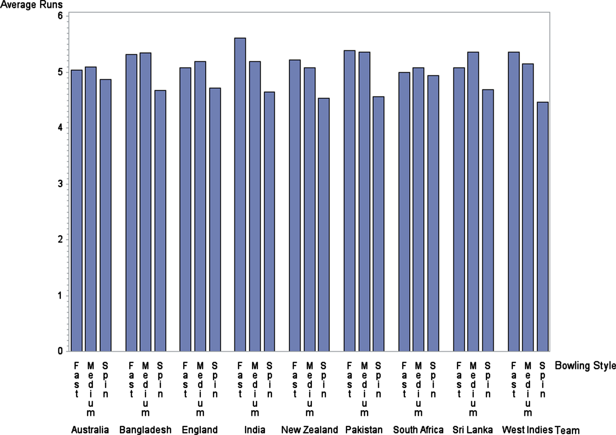
On average, spinners concede the fewest runs per over across all the teams. The average number of runs conceded per over by fast bowlers and medium-fast bowlers are fairly consistent for Australia, Bangladesh, England, New Zealand, Pakistan, and South Africa. For India and the West Indies, fast bowlers conceded the most runs per over, and for Sri Lanka, medium-fast bowlers conceded the most runs per over. Compared to spinners, there is little difference between the runs conceded per over by fast bowlers and medium-fast bowlers among Australia, England, and South Africa. However, these countries have more fast bowlers and fewer medium-fast bowlers than spinners. In contrast, India uses more spinners and fewer fast bowlers compared to medium-fast bowlers. Their fast bowlers conceded more runs per over while their spin bowlers conceded fewer runs per over when compared to their medium-fast bowlers. Additionally, medium-fast bowlers and fast bowlers for New Zealand conceded more runs per over than spin bowlers, on average. Despite these numbers, New Zealand has more fast bowlers and fewer spinners than medium-fast bowlers.
Figure 4 illustrates the variation in runs conceded per over across four stages by the different teams. These teams seem to conceded more runs per over in Stage 4. Apparently most of the teams conceded fewer runs per over in Stage 2. Compared to Stage 2, the average runs conceded per over in Stages 1 and 3 are greater. In contrast, Sri Lanka manages to concede the fewest runs per over, on avarage, in Stage 1, even with the field restrictions imposed during the PowerPlay.
Fig. 4
Average Percentage of Runs Conceded per Over in Each Stage by Different Teams.
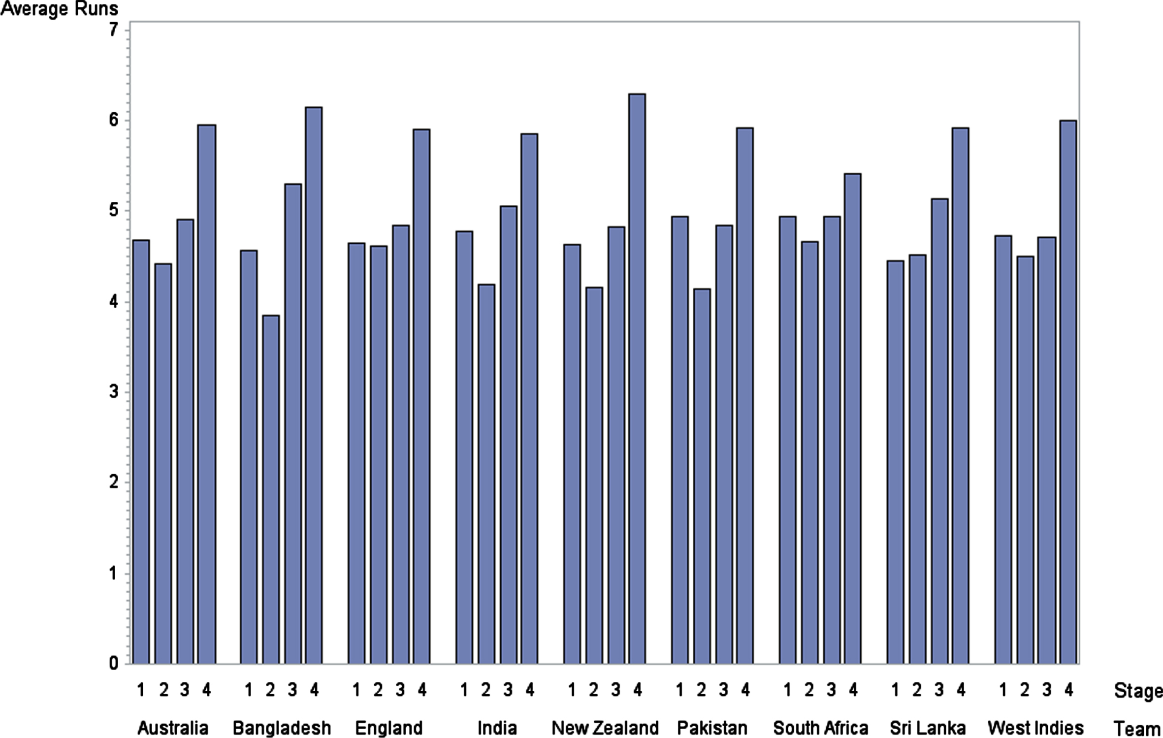
Table 6 summarizes the average percentage of runs conceded per over by the different styles of bowlers across the four stages. On average, spinners conceded the fewest runs per over and this is consistent across all stages. In Stages 2, 3, and 4, medium-fast bowlers conceded more runs per over when compared to both fast bowlers and spinners. For fast bowlers and spinners, Stage 2 is where they conceded the least average percentage of runs per over. Moreover, fast bowlers conceded more runs per over than medium-fast bowlers in Stage 1 while the contrary occurs for the other three stages.
Table 6
Average Percentage of Runs Conceded per Over in Each Stage by Different Types of Bowlers
| Stage | Runs Conceded | ||
| Fast | Medium | Spin | |
| 1 | 4.77 | 4.70 | 4.52 |
| 2 | 4.60 | 4.80 | 4.14 |
| 3 | 4.96 | 5.06 | 4.87 |
| 4 | 5.99 | 6.06 | 5.58 |
As seen, the effect of bowlers across stages varies noticeably among teams. The average runs conceded per over in each stage by each team using different types of bowlers is summarized in Table 8. Table 7 summarizes the percentage of bowlers used in different stages by each team.
Table 8
Average Percentage of Runs Conceded per Over in Each Stage by Each Team Using Different Bowlers
| Team | Runs conceded | |||||||||||
| Stage 1 | Stage 2 | Stage 3 | Stage 4 | |||||||||
| F | M | S | F | M | S | F | M | S | F | M | S | |
| Australia | 4.64 | 4.42 | 5.21 | 4.20 | 4.94 | 4.48 | 5.07 | 4.67 | 4.80 | 5.92 | 5.81 | 6.24 |
| Bangladesh | 4.64 | 4.37 | 4.57 | 4.45 | 4.67 | 3.56 | 5.55 | 5.28 | 5.17 | 6.47 | 6.66 | 5.57 |
| England | 4.64 | 4.80 | 4.10 | 4.67 | 5.11 | 4.45 | 4.75 | 4.92 | 4.87 | 5.93 | 5.84 | 5.78 |
| India | 4.98 | 4.68 | 4.75 | 5.13 | 5.21 | 3.92 | 5.10 | 5.66 | 4.82 | 6.88 | 5.61 | 5.61 |
| New Zealand | 4.76 | 4.55 | 4.16 | 4.64 | 4.31 | 3.77 | 4.60 | 4.97 | 4.87 | 6.47 | 6.32 | 5.67 |
| Pakistan | 5.25 | 4.99 | 4.34 | 4.07 | 4.61 | 4.08 | 4.70 | 5.12 | 4.82 | 6.04 | 6.28 | 5.32 |
| South Africa | 5.02 | 4.47 | 5.48 | 4.26 | 5.09 | 4.70 | 4.73 | 5.17 | 5.02 | 5.36 | 5.58 | 5.27 |
| Sri Lanka | 4.44 | 4.43 | 4.49 | 5.07 | 4.90 | 4.21 | 5.25 | 5.54 | 4.95 | 5.89 | 6.37 | 5.41 |
| West Indies | 4.90 | 4.98 | 4.36 | 5.47 | 4.64 | 4.01 | 5.05 | 4.60 | 4.55 | 6.00 | 6.19 | 5.64 |
| F - Fast Bowlers, M - Medium Fast Bowlers, S - Spinners. | ||||||||||||
Table 7
Percentage of Bowlers Used in Different Stage by Each Team
| Team | Bowling Style | Percentage of Bowlers | Stage | |||
| Stage 1 | Stage 2 | Stage 3 | Stage 4 | |||
| Australia | Fast | 63.48% | 86.61% | 37.05% | 45.71% | 74.64% |
| Medium | 8.93% | 4.76% | 7.59% | 10.71% | 13.21% | |
| Spin | 27.59% | 8.63% | 55.36% | 43.57% | 12.14% | |
| 100.00% | 100.00% | 100.00% | 100.00% | 100.00% | ||
| Bangladesh | Fast | 35.63% | 47.40% | 20.31% | 30.00% | 39.38% |
| Medium | 14.84% | 17.19% | 10.16% | 10.63% | 20.00% | |
| Spin | 49.53% | 35.42% | 69.53% | 59.38% | 40.63% | |
| England | Fast | 54.70% | 79.00% | 25.00% | 32.80% | 71.20% |
| Medium | 17.30% | 16.33% | 16.50% | 16.00% | 20.40% | |
| Spin | 28.00% | 4.67% | 58.50% | 51.20% | 8.40% | |
| India | Fast | 15.13% | 26.75% | 5.26% | 4.74% | 19.47% |
| Medium | 37.37% | 51.75% | 15.79% | 26.84% | 47.89% | |
| Spin | 47.50% | 21.49% | 78.95% | 68.42% | 32.63% | |
| New Zealand | Fast | 39.76% | 53.57% | 25.60% | 27.14% | 47.14% |
| Medium | 34.29% | 37.30% | 30.36% | 30.48% | 37.62% | |
| Spin | 25.95% | 9.13% | 44.05% | 42.38% | 15.24% | |
| Pakistan | Fast | 29.71% | 40.38% | 8.17% | 19.62% | 44.23% |
| Medium | 24.13% | 36.22% | 10.58% | 15.38% | 29.23% | |
| Spin | 46.15% | 23.40% | 81.25% | 65.00% | 26.54% | |
| South Africa | Fast | 55.13% | 77.50% | 28.13% | 38.50% | 66.50% |
| Medium | 20.88% | 18.33% | 21.88% | 20.50% | 23.50% | |
| Spin | 24.00% | 4.17% | 50.00% | 41.00% | 10.00% | |
| Sri Lanka | Fast | 42.98% | 64.18% | 16.49% | 24.68% | 57.02% |
| Medium | 20.53% | 17.02% | 23.40% | 18.30% | 24.68% | |
| Spin | 36.49% | 18.79% | 60.11% | 57.02% | 18.30% | |
| West Indies | Fast | 37.11% | 44.07% | 22.78% | 28.44% | 48.89% |
| Medium | 29.67% | 21.48% | 26.11% | 38.22% | 33.78% | |
| Spin | 33.22% | 34.44% | 51.11% | 33.33% | 17.33% | |
In cricket every team gets the opportunity to use a new ball at the beginning of an innings. Depending on field conditions, fast and medium-fast bowlers may be able to swing a new ball at a fast pace. Consequently, it is a common practice of the bowling team to start its 20 over innings with fast bowlers or medium-fast bowlers. When a ball swings, it is usually difficult for a batsmen to judge its trajectory, and there is a tendency to play poor shots. So, when combined with swing and pace, a bowling team should try to get a few quick wickets at the early stages of a match. This creates pressure on the batting team, forcing it towards a lower total. This phenomenon causes a team to use fast and medium-fast bowlers more frequently in Stage 1, as demonstrated in Table 7. Nonetheless, there are situations where some teams begin with a spinner for an orthodox start.
As a match progresses, the ball becomes tattered and it is easier for spinners to spin the ball. So, teams tend to introduce spinners in Stage 2, as seen in Table 7. During Stage 4 it is common for batsmen to attempt riskier shots so as (i) to accumulate additional runs to reach a target set by the opposing team, or (ii) to set a higher target for the opposing team. A common practice for a bowling team to use its best fast bowlers in the last few overs of an innings. The idea behind this strategy is to use a bowler’s pace and pitching experience to target areas most likely to prevent batsman from scoring runs, or even forcing batsmen to attempt poor shots, causing them to be more vulnerable to sacrificing wickets.
Usually a balanced team consists of two or three spinners, two or three fast and medium-fast bowlers, and five or six batsmen. A balanced team allows the captain considerable flexibility for using the most effective bowler in a given stage of the match. For example, the subsequent paragraphs describe insights into the bowling strategies used by India, New Zealand, and England.
For India, Table 8 shows the fewest runs conceded per over are from spinners during Stages 2 and 3. In Stage 4, the runs conceded per over by both medium-fast bowlers and spinners are the same, and lower than the runs conceded per over by fast bowlers. Fast bowlers conceded the most runs per over in Stage 1, while medium-fast bowlers conceded the least. India uses more medium-fast bowlers in Stages 1 and 4, and more spinners in Stages 2 and 3, as seen in Table 7. Furthermore, as fast bowlers conceded more runs per over in both Stages 1 and 4 when compared to other stages, India uses relatively fewer fast bowlers in Stages 1 and 4. In summary, it seems that India uses its bowlers effectively, given that it has more spinners and fewer fast bowlers than medium-fast bowlers, as shown in Figure 2.
From Table 7, New Zealand uses more fast bowlers and fewer spinners in Stages 1 and 4 when compared to medium-fast bowlers. In Stage 3, New Zealand uses fewer fast bowlers compared to other bowling styles. In contrast, New Zealand’s fast bowlers conceded the most runs per over during Stages 1 and 4, and the least in Stage 3, as seen in Table 8. Furthermore, spinners conceded the fewest runs per over in Stages 1 and 4; however, New Zealand uses fewer spinners in Stages 1 and 4, compared to other bowling styles.
For England, fast bowlers conceded the most runs per over in Stage 4 and spinners conceded the least, as shown in Table 8. In Stage 3, the smallest average percentage of runs conceded per over occurs with fast bowlers, and the most conceded is from medium-fast bowlers. Nevertheless, England uses more fast bowlers and fewer spinners in Stage 4, yet more spinners in Stage 3.
We next model, using both OLS and QR, the Percentage of Runs Conceded Per Over as the dependent variable with respect to the independent variables of Stage and Bowling Style.
3.1Ordinary least squares model
For the Ordinary Least Squares (OLS) linear regression model, the behavior of the conditional mean of a response variable, based on one or more explanatory variables, is investigated. OLS estimators are consistent and optimal within the class of linear, unbiased estimators, whenever the errors are homoscedastic and serially uncorrelated (Hayes and Cai (2007)).
As described earlier in this study, the Percentage of Runs Conceded per Over is considered as the response variable and Stages (1, 2, 3, 4) and Bowling Style (fast, medium-fast, spin) are the two predictor variables. During Stage 3, which consists of overs eleven through fifteen, the game usually progresses smoothly. Hence, for the Stages predictor variable, Stage 3 is used as a reference category. Likewise, the medium-fast bowling style is used as the reference category for the Bowling Style predictor variable. A summary of OLS regression results is provided in Table 9.
Table 9
Ordinary Least Square (OLS) Model (Overall)
| Effect | Estimate | Srandard Error | t Value | Pr >|t| |
| Intercept | 5.1249 | 0.08132 | 63.02 | < .0001 |
| Stage 1 | -0.3280 | 0.08218 | -3.99 | < .0001 |
| Stage 2 | -0.5493 | 0.08744 | -6.28 | < .0001 |
| Stage 4 | 0.8968 | 0.08497 | 10.55 | < .0001 |
| Stage 3 | 0 | . | . | . |
| Fast Bowling | -0.0497 | 0.07605 | -0.65 | 0.5131 |
| Spin Bowling | -0.3437 | 0.08142 | -4.22 | < .0001 |
| Medium Fast Bowling | 0 | . | . | . |
Relative to Stage 3, Table 9 shows the percentage of runs conceded per over in Stages 1, 2, and 4 are statistically significant. The percentage of runs conceded per over by fast bowlers is not significant relative to medium-fast bowlers, but for spinners it is significant at the 5% significance level. Also, relative to Stage 3, Stage 1 and Stage 2 bowlers have conceded the smallest percentage of runs per over. On the other hand, the results show that the percentage of runs conceded per over in Stage 4 is significantly higher when compared to that in Stage 3. Note that the OLS regression model can only explain the effect of the predictors with respect to the conditional mean. In practice, it would also be useful to know the effects of the predictors at different quantiles as well. For example, a team captain can assess the risk and decide the type of the bowler to be used in a particular over by looking at a regression model that explains the 0.9 quantile of the percentage of runs conceded per over. This cannot be accomplished using an OLS model; however, a quantile regression model is capable of providing valid inferences for all quantiles. Using quantile regression to model bowling effectiveness, along with some key results concerning this model, is discussed in the next section.
3.2Quantile regression models
In this section, we use Quantile Regression (QR) to model the Percentage of Runs Conceded per Over with respect to the independent variables Stage and Bowling Style. To facilitate comparisons, Table 10 gives parameter estimates and significance results for three QR models: 0.25, 0.50, and 0.75. Graphical representations for the effect plots over the entire quantile spectrum are presented in Figure 5 for a more comprehensive view.
Table 10
Quantile Regression Model (Overall)
| Effect | At 0.25 Quantile | At 0.50 Quantile | At 0.75 Quantile |
| Estimate P-Value | Estimate P-Value | Estimate P-Value | |
| Intercept | 3.3613 | 4.8738 | 6.6152 |
| < .0001 | < .0001 | < .0001 | |
| Stage 1 | -0.5566 | -0.3039 | -0.1515 |
| < .0001 | 0.0043 | 0.1971 | |
| Stage 2 | -0.3540 | -0.5801 | -0.6870 |
| < .0001 | < .0001 | < .0001 | |
| Stage 4 | 0.4297 | 0.8381 | 1.2060 |
| 0.0002 | < .0001 | < .0001 | |
| Stage 3 | Reference | ||
| Fast Bowling | -0.0873 | -0.1119 | -0.0459 |
| 0.3029 | 0.2595 | 0.6122 | |
| Spin Bowling | -0.3930 | -0.4177 | -0.4637 |
| < .0001 | < .0001 | < .0001 | |
| Medium Fast Bowling | Reference | ||
Fig. 5
Quantile Process Plots for Estimated Parameters with 95% Confidence Interval.
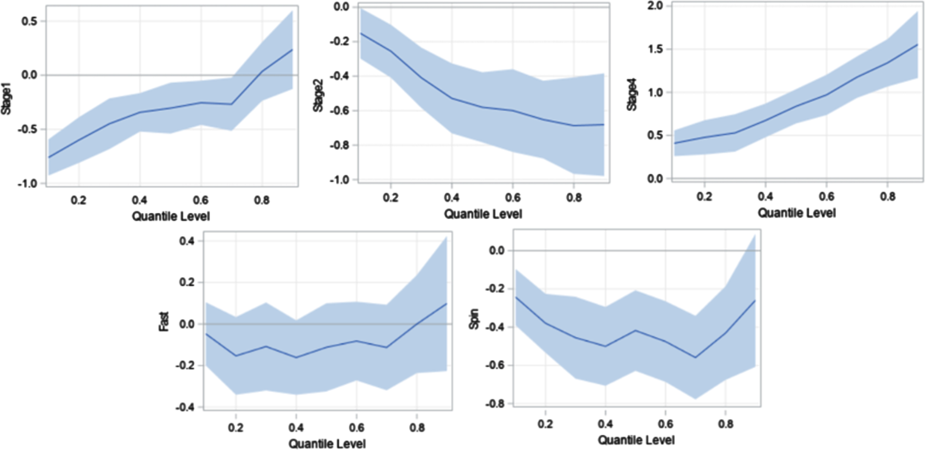
Table 10 results demonstrate noticeable differences in the parameter estimates of the effects of the factors at different quantiles. It provides the differing effects of the Stage and Bowling Style factors at pre-specified quantiles of the Percentage of Runs Conceded per Over. However, the OLS model is incapable such conclusions since it provides inferences only for the conditional mean. For example, at the 0.25 quantile, and relative to the Stage 3 baseline, there is a decrease of 0.56 percentage points in the number of runs per over conceded in Stage 1. As mentioned earlier, the results shown throughout this study are based on the percentage points of total runs conceded per over. Of course, it is simple to convert these percentages to raw numbers of runs (e.g. 0.56 percentage in a match with 264 total runs is 1.48 raw actual runs). In contrast, at the 0.75 quantile, and relative to the Stage 3 baseline, there is only a decrease of 0.15 percentage points in the number of runs conceded per over in Stage 1, which is not statistically significant. Relative to the Stage 3 baseline, in Stage 2 bowlers have conceded 0.35 percentage points fewer at the 0.25 quantile, while this figure rises to 0.69 percentage points fewer at the 0.75 quantile, and to 0.58 percentage points fewer at 0.50 quantile.
Results in Table 10 further demonstrate that spinners concede fewer runs per over when compared to the medium-fast bowlers, and the effect is statistically significant for all three quantiles. Additionally, for all three quantiles, there is no significant difference between fast bowlers and medium-fast bowlers with respect to the number of runs conceded per over. This result is consistent with the OLS model as well. However, for the 0.75 quantile model, and when compared to Stage 3, it is important to note that the effect of Stage 1 is not statistically significant at the 5% significance level, but the OLS results indicate that the effect during Stage 1 is statistically significant. Bear in mind that OLS only models the conditional mean of the response variable.
Plots of the changes to the effect of the predictors (regression coefficients) as the quantile level moves from lower quantiles, near 0.1 to upper quantiles, near 0.9, are shown in Figure 5. The model effect of Stage 1 is increasing steadily as the quantile level changes from lower to upper. A change in the sign of the effect near the 0.8 quantile suggests that relative to Stage 3, the Stage 1 bowlers have conceded fewer runs per over at quantile levels less than the 0.8 quantile value, and conceded more runs per over at quantile levels greater than the 0.8 quantile value, even though the latter is not statistically significant. In other words, when considering low-scoring situations (lower quantiles), bowlers concede fewer runs per over in Stage 1 than in Stage 3. However, for high-scoring situations (upper quantiles), the number of runs conceded per over in Stage 1 is greater when compared to that in Stage 3. The effect of Stage 2 is decreasing steadily as the quantile level increases, and it is significant throughout the entire spectrum of all quantiles. This implies that in Stage 2, bowlers concede fewer runs per over than in Stage 3; it is also seen that this difference increases as the quantile level increases. Similar to the descriptive analysis discussed earlier, bowlers concede significantly more runs per over in Stage 4, when compared to Stage 3, across all quantiles.
Additionally, Table 10 shows that the number of runs conceded per over by fast bowlers is not significant when compared to medium-fast blowers, and this is consistent across all the quantiles. In contrast, spinners conceded fewer runs per over than medium-fast bowlers, and this is also consistent across all quantiles. Apparently, this difference is greater for quantiles in the middle range of (0.1, 0.9).
To investigate whether there is a difference in the results shown above across different teams, QR modeling was repeated for individual teams. Those results were quite consistent, barring a few exceptions. Figures 6a, 6b, and 6c show quantile process plots of the effects (regression coefficients) of the predictors for each team. These plots indicate that the results for individual teams are mostly consistent, with the graphs being based on the full data set associated with Figure 5.
Fig. 6a
Quantile Process Plots for Estimated Parameters with 95% Confidence Bands for Australia, Bangladesh, and England.
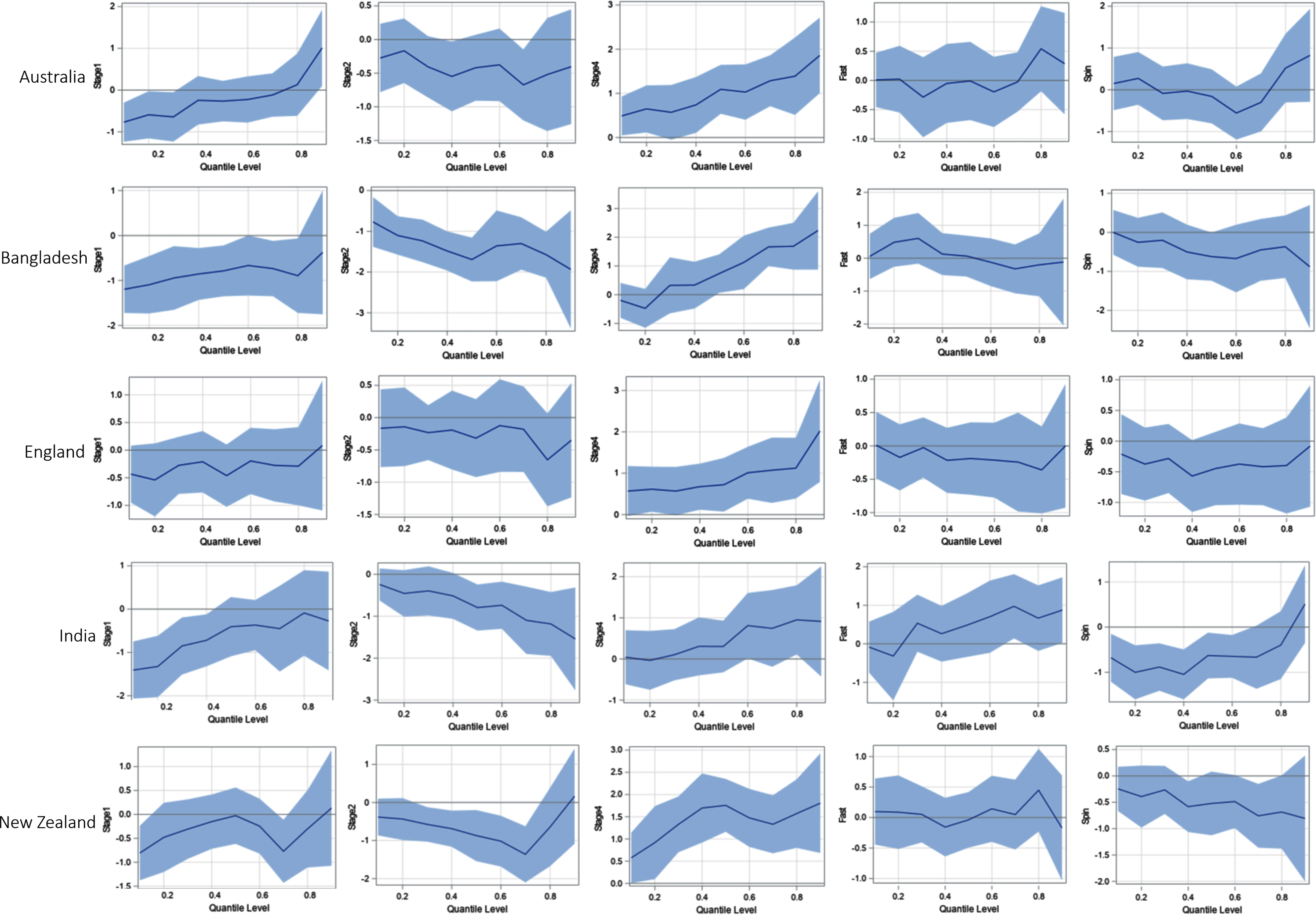
Fig. 6b
Quantile Process Plots for Estimated Parameters with 95% Confidence Bands for Australia, Bangladesh, and England.
The quantile plot for Stage 1 is steadily increasing for most of the countries, while the quantile plot for Stage 2 is generally decreasing for most of the countries. The signs of the effects being negative for these two stages indicate that the runs conceded per over in Stages 1 and 2 are relatively lower than that in State 3. In contrast, the plots for Stage 4 are steadily increasing and the sign of that effect is positive. This indicates that, relative to Stage 3, in Stage 4 bowlers conceded more runs per over. In general, this phenomenon is somewhat consistent across the individual teams. Spinners concede fewer runs per over than medium-fast bowlers; but when compared to medium-fast bowlers, there is no significant difference in the number of runs per over conceded by fast bowlers. These bowling style effects are also mostly consistent among all teams.
Notice that there are a few cases where the results for individual teams were somewhat different from the pattern in the overall model that was based on the full data set associated with Figure 5. For example, Figure 5 shows that the overall effect of Stage 1 changes its sign near the 0.8 quantile; but, as shown in Figure 6a and 6b, for the countries South Africa, Pakistan, and West Indies, the sign of the effect changes near the 0.60, 0.40, and 0.25 quantiles, respectively. Furthermore, even though the effect is not significant, and contrary to the overall pattern in Figure 5, Indian and West Indies fast bowlers seem to concede more runs per over than their medium-fast bowlers.
4Bayesian quantile regression
In this section we offer a Bayesian approach to quantile regression for modeling bowling effectiveness. Yu and Moyeed (2001) introduced the possibility of using a likelihood function based on the asymmetric Laplace distribution for Bayesian Quantile Regression (BQR). They argue that using an asymmetric Lapalace distribution is a more natural and effective way to model when considering BQR. Naturally, the Markov Chain Monte Carlo (MCMC) procedure is used to empirically approximate the posterior distributions. The probability density function for the asymmetric Laplace distribution used here has the form
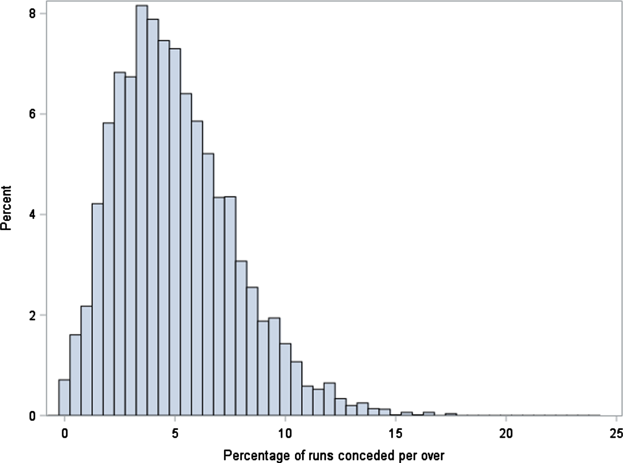
A histogram of the response variable, the percentage of runs conceded per over, is provided in Figure 7, where this marginal distribution is seen to be asymmetric and right-skewed.
Fig. 7
Distribution of Percentage of Runs Conceded Per Over.
The BQR model studied here is
Figure 8 shows the trace plots, autocorrelation plots, and the kernel density estimates of the parameters β0 (p) , β1 (p), β2 (p), β3 (p), β4 (p), and β5 (p), respectively, for the 0.50 quantile. Figures 11 and 12 in the Appendix provide similar plots for the 0.25 and 0.75 quantiles. The kernel density estimates for all six parameters are relatively unimodal and smooth. But, the autocorrelation plots show evidence of non-negligible autocorrelation in the posterior samples, which is usually an indication of slow mixing.
Fig. 8
MCMC Diagnostic Plots At 0.50 Quantile.

Fig. 11
MCMC Diagnostic Plots At 0.25 Quantile.
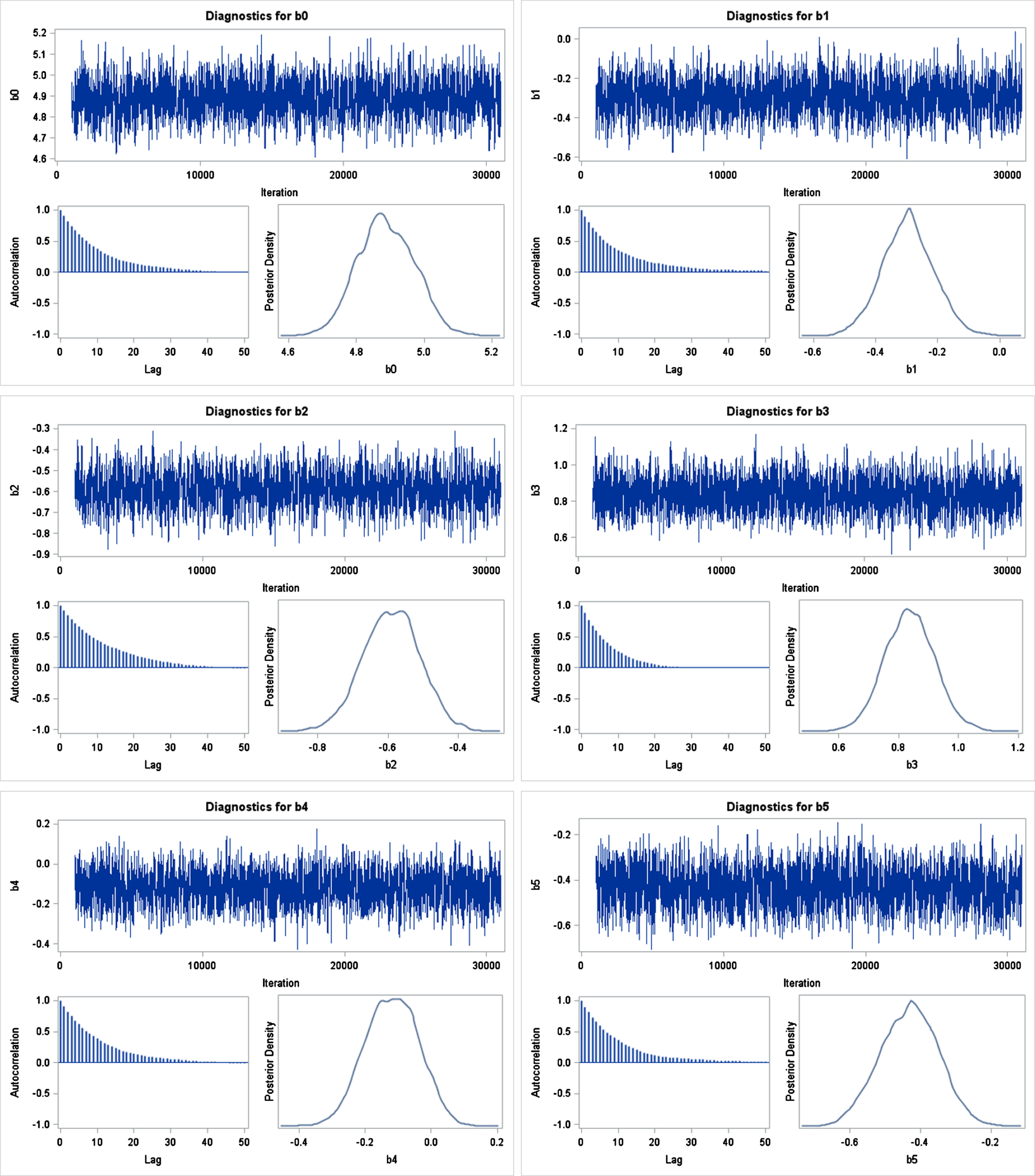
Fig. 12
MCMC Diagnostic Plots At 0.75 Quantile.
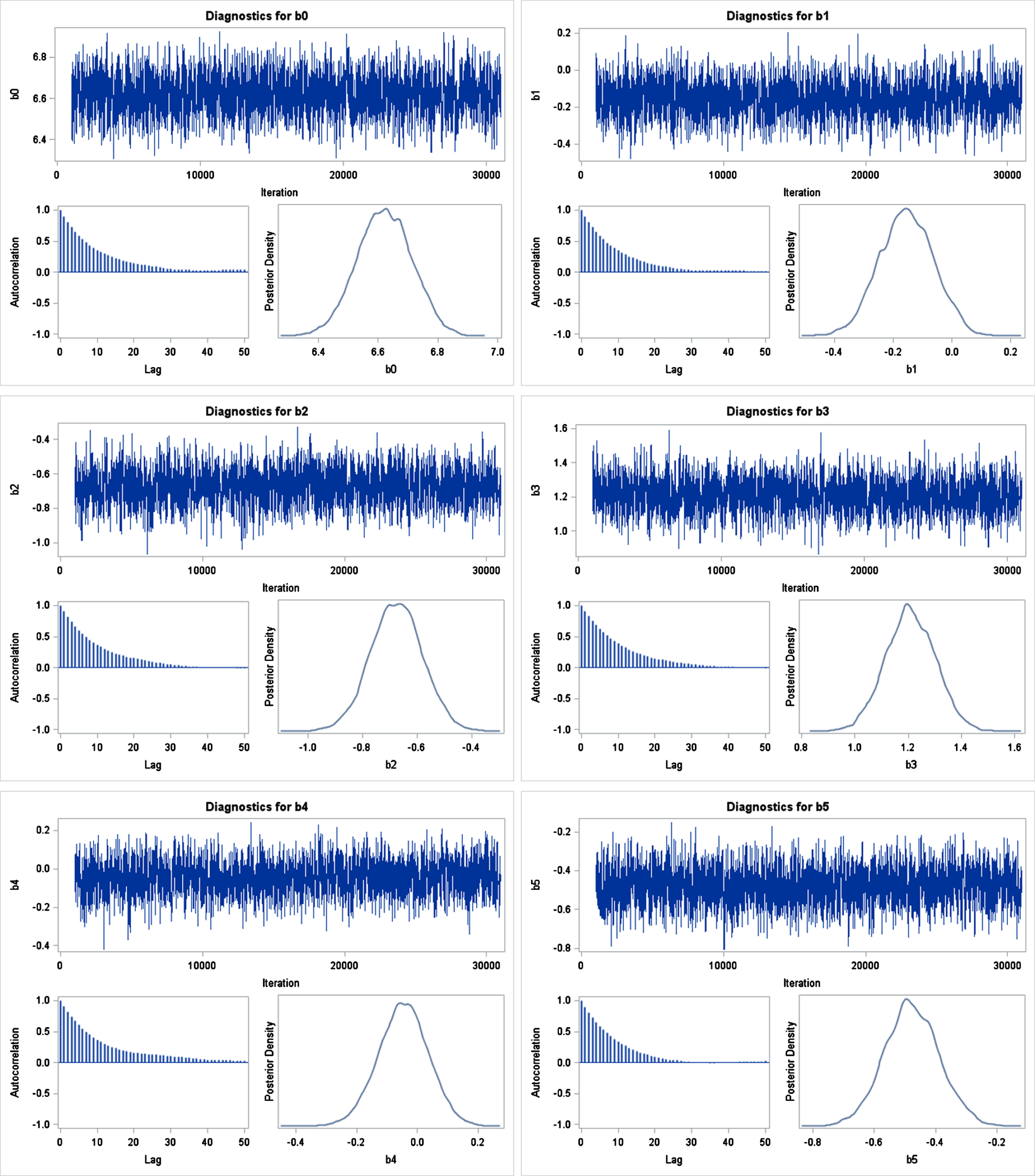
Table 11 provides Monte Carlo Standard Errors (MCSE) for each model parameter. The errors are small relative to the posterior standard deviations (SD), and small MSCE/SD ratios are indications that the Markov Chain has stabilized and the mean estimates do not vary much over time.
Table 11
Monte Carlo Standard Errors (MCSE) at 0.50 Quantile
| Parameter | MCSE | Standard Deviation | MCSE/SD |
| β0 | 0.0022 | 0.0832 | 0.0259 |
| β1 | 0.0022 | 0.0830 | 0.0266 |
| β2 | 0.0023 | 0.0804 | 0.0280 |
| β3 | 0.0018 | 0.0832 | 0.0217 |
| β4 | 0.0021 | 0.0806 | 0.0260 |
| β5 | 0.0021 | 0.0817 | 0.0260 |
As was accomplished in the previous section, it is useful to examine the quantile process, or how the estimated regression parameters for each covariate change as the quantile p varies over the interval (0, 1). Specifically, the quantile levels 0.1 to 0.9 are used with increments of 0.10. Figure 9 shows the quantile process plots for the estimated parameters except for the intercept term (β0), and the corresponding quantile parameter estimates are given in Table 12. The results show that the parameter estimates tend to vary widely around the particular quantile of interest. Throughout the process, β2 and β5 are negative. For β1, the 95% HPD (Highest Posterior Density) interval is negative throughout most of the process; and beyond the 0.70 quantile those intervals contain 0. In contrast, the process contains zero for all the quantiles except the 0.40 quantile for β4. For β3, the 95% HPD interval is positive throughout the process.
Fig. 9
Bayesian Quantile Process Plots for Estimated Parameters with 95% HPD Interval.
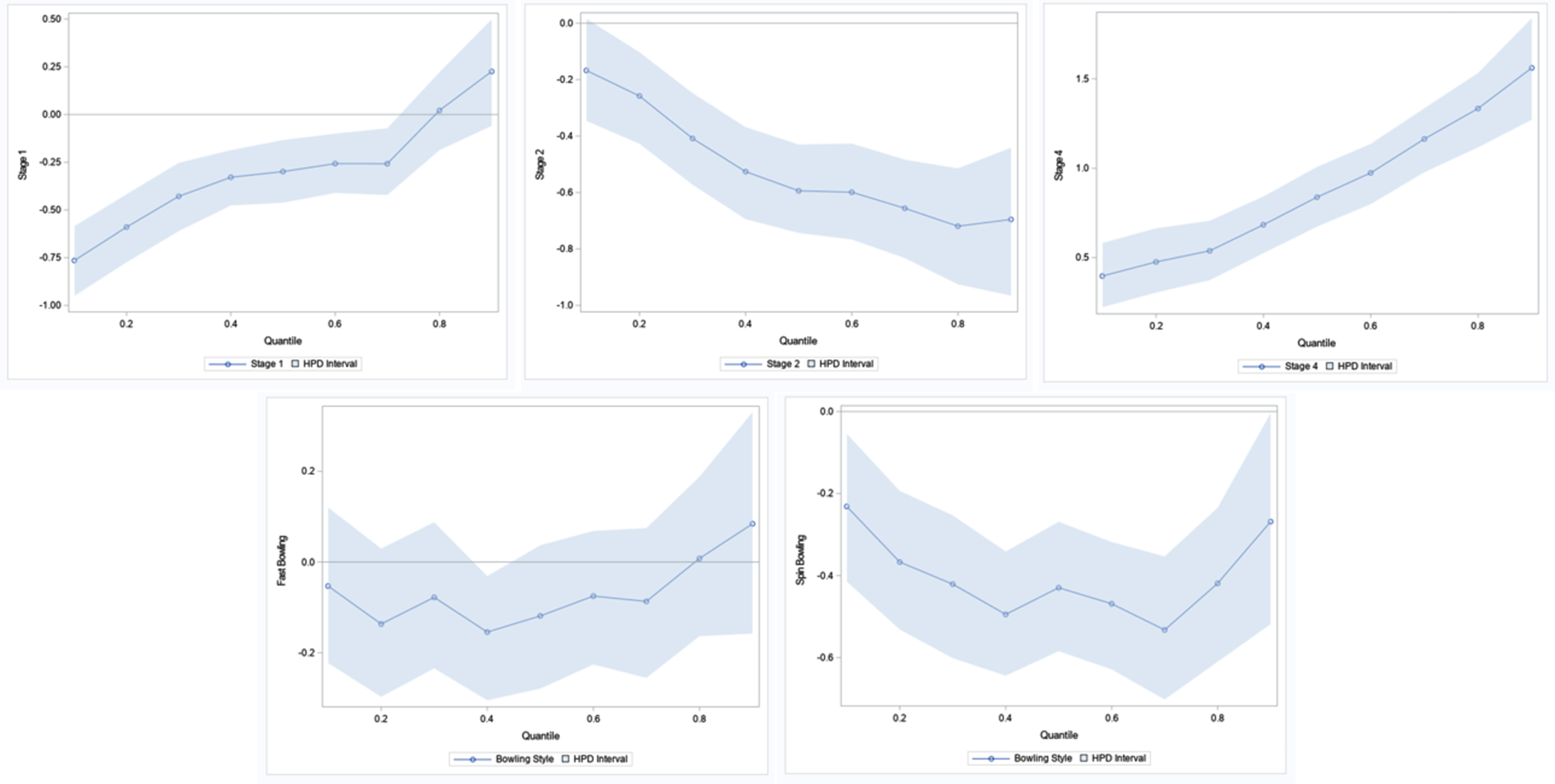
Table 12
Quantile Process Table For Estimated Parameters with 95% HPD Interval
| p | β1 | β2 | β3 | ||||||
| Mean | HPD Lower | HPD Upper | Mean | HPD Lower | HPD Upper | Mean | HPD Lower | HPD Upper | |
| 0.1 | -0.7644 | -0.9498 | -0.5844 | -0.1674 | -0.3462 | 0.0163 | 0.3971 | 0.2224 | 0.5823 |
| 0.2 | -0.5894 | -0.7740 | -0.4175 | -0.2578 | -0.4272 | -0.1026 | 0.4762 | 0.3047 | 0.6643 |
| 0.3 | -0.4285 | -0.6107 | -0.2526 | -0.4083 | -0.5723 | -0.2475 | 0.5383 | 0.3743 | 0.7068 |
| 0.4 | -0.3287 | -0.4766 | -0.1866 | -0.5259 | -0.6944 | -0.3681 | 0.6837 | 0.5247 | 0.8422 |
| 0.5 | -0.2989 | -0.4621 | -0.1331 | -0.5938 | -0.7433 | -0.4294 | 0.8384 | 0.6735 | 1.0080 |
| 0.6 | -0.2569 | -0.4107 | -0.1002 | -0.5988 | -0.7664 | -0.4263 | 0.9741 | 0.7996 | 1.1368 |
| 0.7 | -0.2575 | -0.4215 | -0.0716 | -0.6557 | -0.8323 | -0.4831 | 1.1639 | 0.9776 | 1.3359 |
| 0.8 | 0.0213 | -0.1867 | 0.2218 | -0.7193 | -0.9255 | -0.5143 | 1.3345 | 1.1171 | 1.5336 |
| 0.9 | 0.2255 | -0.0592 | 0.4984 | -0.6953 | -0.9653 | -0.4411 | 1.5614 | 1.2716 | 1.8396 |
| p | β4 | β5 | |||||||
| Mean | HPD Lower | HPD Upper | Mean | HPD Lower | HPD Upper | ||||
| 0.1 | -0.0528 | -0.2228 | 0.1205 | -0.2314 | -0.4145 | -0.0540 | |||
| 0.2 | -0.1364 | -0.2970 | 0.0298 | -0.3669 | -0.5315 | -0.1933 | |||
| 0.3 | -0.0777 | -0.2343 | 0.0880 | -0.4208 | -0.6012 | -0.2530 | |||
| 0.4 | -0.1542 | -0.3046 | -0.0308 | -0.4945 | -0.6441 | -0.3410 | |||
| 0.5 | -0.1186 | -0.2789 | 0.0371 | -0.4296 | -0.5842 | -0.2686 | |||
| 0.6 | -0.0750 | -0.2258 | 0.0688 | -0.4686 | -0.6287 | -0.3180 | |||
| 0.7 | -0.0867 | -0.2552 | 0.0751 | -0.5324 | -0.7020 | -0.3530 | |||
| 0.8 | 0.0080 | -0.1634 | 0.1883 | -0.4189 | -0.6100 | -0.2345 | |||
| 0.9 | 0.0844 | -0.1577 | 0.3305 | -0.2684 | -0.5184 | -0.0038 | |||
Table 12 provides HPD intervals for the range of quantiles studied here. The coefficient β1 is steadily increasing as the quantile level increases from lower quantiles to upper quantiles. Furthermore, that coefficient changes its sign near the 0.80 quantile. This indicates that relative to Stage 3, in Stage 1 bowlers concede fewer runs per over for quantiles below 0.80, but changes to conceding more runs per over for quantiles above 0.80. The effects plots in Figure 9 confirm this relationship. Recall that this same conclusion was reached using the non-Bayesian approach of
the previous section. The coefficient β 2 is steadily decreasing as the level of quantile increases from lower quantiles to upper quantiles. So, relative to Stage 3, in Stage 2 bowlers concede fewer runs per over throughout the entire spectrum of quantiles, and this effect is greater for higher quantiles. For example, the decrease in the percentage of runs conceded per over in Stage 2, when compared to Stage 3, is 0.2578 for the 0.2 quantile, and it is 0.7193 for the 0.8 quantile. Again, this outcome is also consistent with the non-Bayesian analysis previously presented. The coefficient β 3 steadily increases as the quantile level increases from lower quantiles to upper quantiles. This indicates that relative to Stage 3, in Stage 4 bowlers concede more runs per over throughout the entire spectrum of the quantiles. Additionally, this effect gradually becomes larger as one views from lower quantiles to upper quantiles. For example, the increase in the percentage of runs conceded per over in Stage 4, when compared to Stage 3, is 0.4762 for the 0.2 quantile and it rises to 1.3345 for the 0.8 quantile. The coefficient β 4 is not significant for all quantiles except those near 0.40. Even though this effect is not significant, having a negative coefficient for most of the quantiles indicates that fast bowlers concede fewer runs per over than medium-fast bowlers. This is also consistent with the outcome of our non-Bayesian approach. Finally, the coefficient β 5 is significant and negative for all the quantiles. This indicates that relative to medium-fast bowlers, spinners tend to concede fewer runs per over; and this difference is greater for lower and upper quantiles, while smaller for the middle quantiles. As before, this outcome is consistent with our previous non-Bayesian analysis.
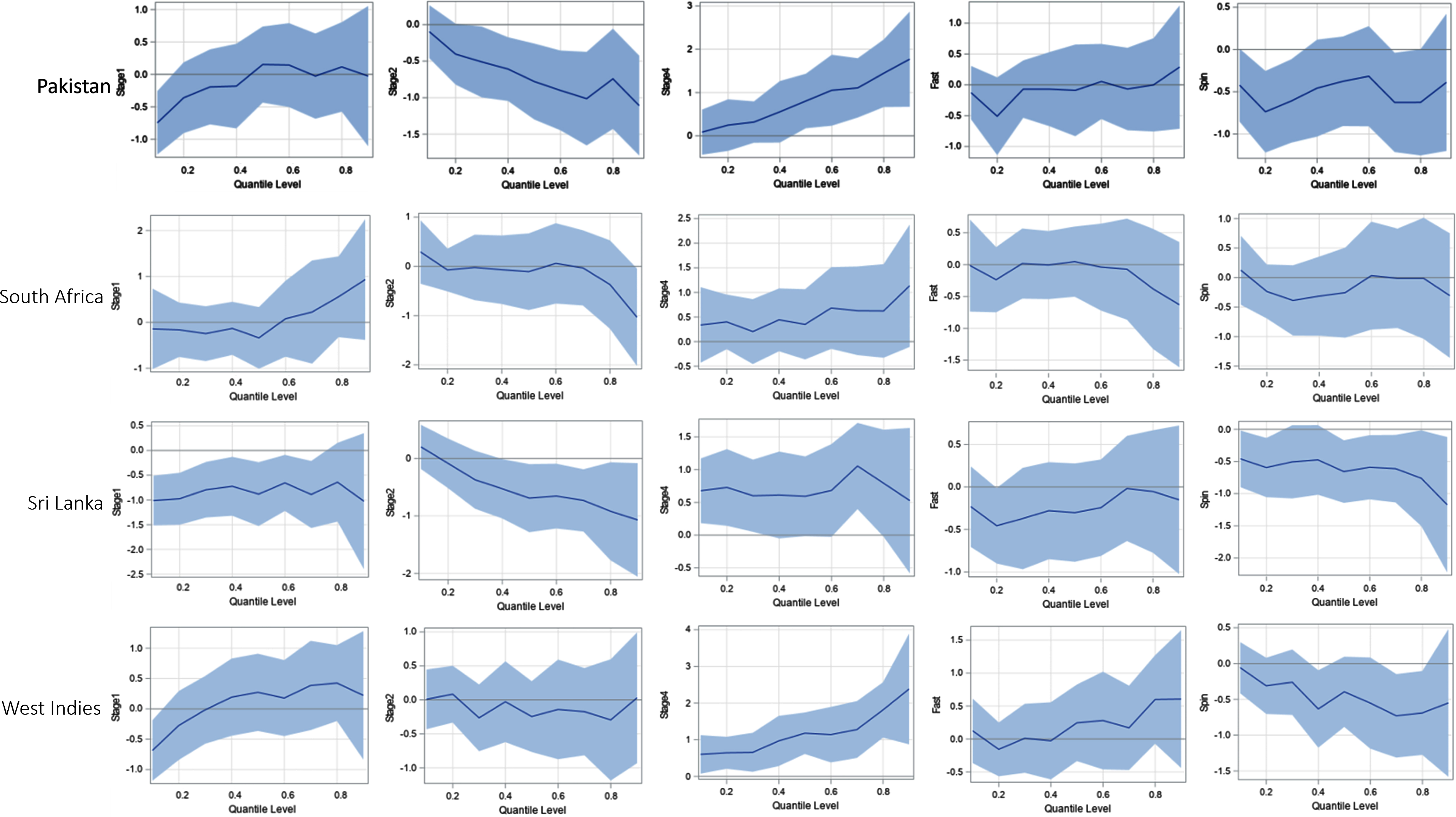
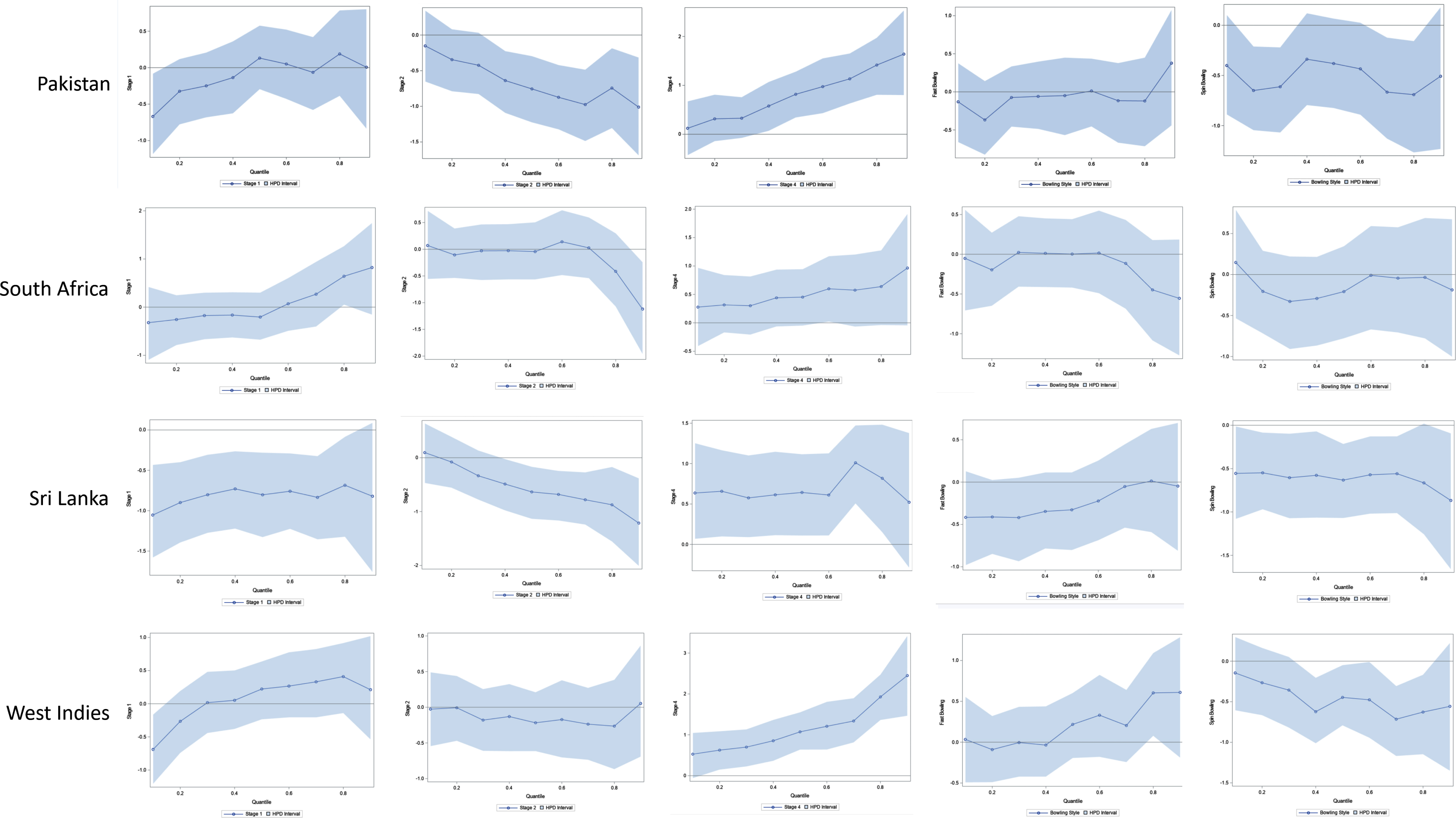
In summary, the quantile plots of the regression coefficients in Figure 9 using the BQR approach are similar to the plots in Figure 5. This confirms that the outcome of the BQR analysis is consistent with the usual QR analysis discussed in the previous section. For completeness, similar plots were also derived for individual ICC teams and are given in Figures 10a, 10b, and 10c. These plots are similar to those shown in Figures 6a, 6b, and 6c, again showing consistency with the usual QR approach.
Fig. 10a
Bayesian Quantile Process Plots for Estimated Parameters with 95% HPD Interval for Australia, Bangladesh, and England.
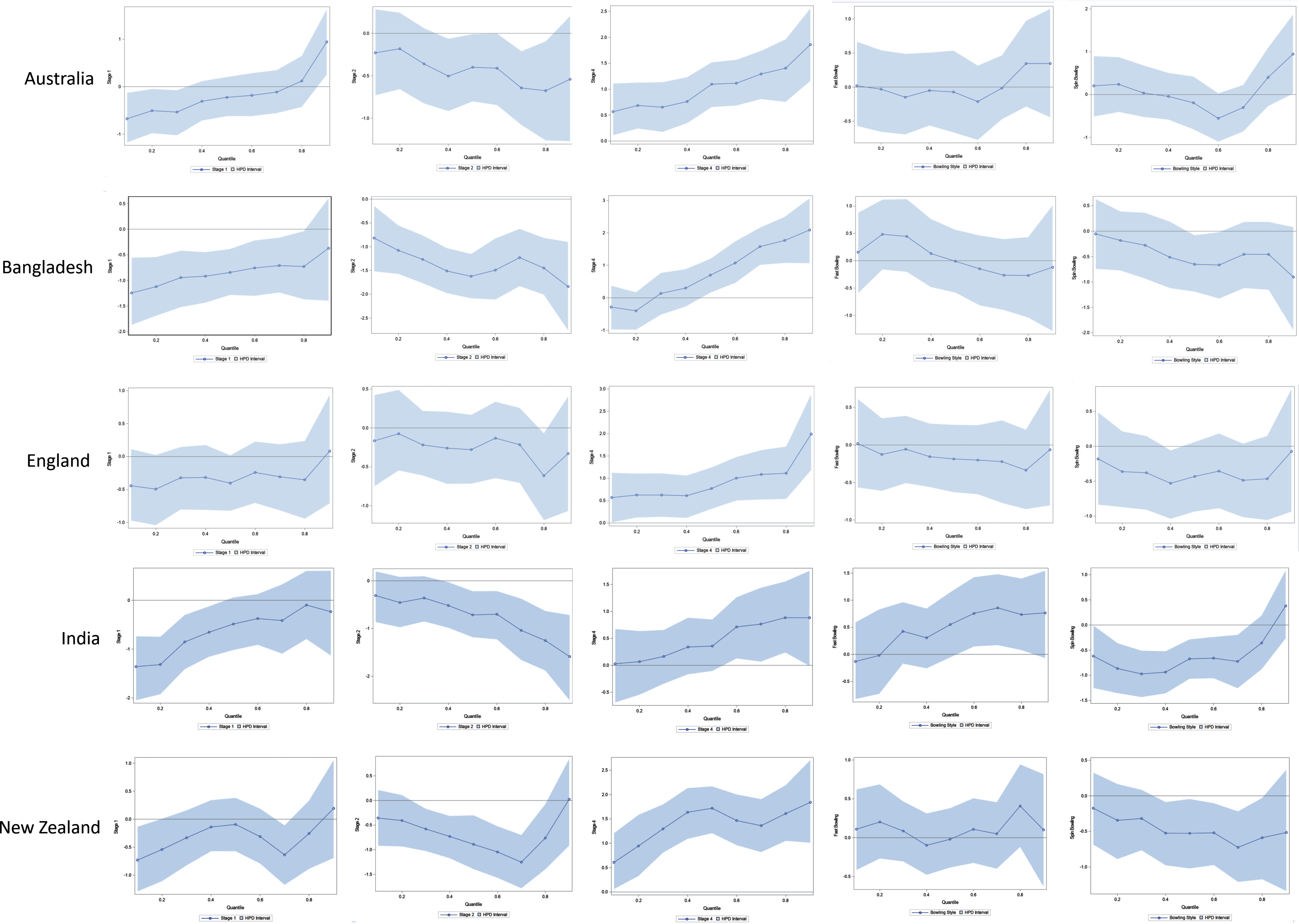
Fig. 10b
Bayesian Quantile Process Plots for Estimated Parameters with 95% HPD Interval for India, New Zealand, and Pakistan.
5Discussion and conclusions
This article has shown that quantile regression can effectively be used to model the bowling performance of T20I cricket. In addition, a Bayesian-type extension to the same model has also been studied. For modeling purposes, the twenty over innings of a T20I match was divided into four stages: Stage 1 (overs 1-6 PowerPlay), Stage 2 (overs 7-10), Stage 3 (overs 11-15), and Stage 4 (overs 16-20). Additionally, bowlers were partitioned into three separate types: fast bowlers, medium-fast bowlers, and spinners. Given that ordinary least squares (OLS) regression can only model the conditional mean of the response variable, we have shown the relevance of quantile regression in modeling the entire spectrum of the distribution of the response variable. To alleviate other effects, like environmental conditions and ground effects, the percentage of runs conceded per over has been used as the response variable, instead of simply runs per over. As a result, greater insight into the effects of the predictors throughout the entire spectrum of quantiles is gained, which would not be possible to accomplish using the usual OLS model. Not having to fulfill the assumptions of normality and homoscedasticity, combined with robustness to the presence of outliers, are principal reasons why practitioners tend to prefer quantile regression over OLS regression. We have also employed a Bayesian framework to the quantile regression problem as a means of confirming the findings. A considerably large data set, which includes 8040 overs from the T20I matches played up to May 2019, has been used in these analyses.
There are several key findings in this study. Relative to Stage 3, bowlers have conceded more runs per over in Stage 1, and this difference appears to be decreasing with the quantile level of the response variable. Similarly, in Stage 2, bowlers have conceded fewer runs per over than in Stage 3, and this difference is increasing with the quantile level of the runs conceded per over. When compared to Stage 3, bowlers have conceded more runs per over in Stage 4 and this difference is more pronounced in the upper quantiles. With respect to Bowling Styles, when compared to medium-fast bowlers, spinners have conceded fewer runs per over, and this disparity is more visible for quantiles in the middle range. There is no significant difference between the number of runs conceded per over for fast bowlers when compared to medium-fast bowlers. Based on the results from the individual country models, it is noted that these patterns are consistent for most of the ICC teams, but with a few exceptions. Results obtained from the Bayesian framework were also consistent with those of the non-Bayesian approach studied here. To see if a difference in the effectiveness of bowling styles during different stages of the match was detectable, revised models including interactions terms were studied. However, these interaction terms were not statistically significant except in a very few cases, so that effort proved fruitless.
In conclusion, this study has demonstrated the usefulness of the quantile regression approach for evaluating the performance of bowlers in the game of cricket. The findings here can be useful for cricket administrators, team managers, and captains pursuing an effort to mobilize their bowlers effectively. Because this study considered only one key aspect of the bowler performance, runs conceded per over, other avenues remain open for investigation. Future research will incorporate another key aspect of bowling performance: the number of wickets taken per over, which is a natural extension of this work.
6Appendix
Leibnitz Rule: Let f (θ, x) be a real-valued function such that it and its partial derivative fθ (θ, x) are continuous in θ and x in some region R of the (θ, x) plane, including a (θ) ≤ x ≤ b (θ), θ0 ≤ θ ≤ θ1, where a (θ) and b (θ) are both continuous, with continuous derivatives, on [θ0, θ1] as well. Then, for θ ∈ [θ0, θ11]
Proposition. As a function of
Proof. Define
Therefore,
Table 13 shows the Effective Sample Sizes. The autocorrelation times for the three parameters range from 14.18 to 23.45 and the efficiency rates are low. These results account for the relatively small effective sample sizes, given a nominal sample size of 30, 000.
Table 13
Effective Sample Size (ESS) at 0.50 Quantile
| Parameter | ESS | Autocorrelation Time | Efficiency |
| β0 | 1493.7 | 20.0846 | 0.0498 |
| β1 | 1416.4 | 21.1806 | 0.0472 |
| β2 | 1279.1 | 23.4548 | 0.0426 |
| β3 | 2115.4 | 14.1818 | 0.0705 |
| β4 | 1484.4 | 20.2099 | 0.0495 |
| β5 | 1477.3 | 20.3069 | 0.0492 |
References
1 | Akhtar, S. , Scarf, P. and Rasool, Z. , (2015) , Rating players in test match cricket, Journal of the Operational Research Society, 66: (4), 684–695. |
2 | Benoit, D. F. and Van den Poel, D. , (2017) , bayesQR: A Bayesian approach to quantile regression, Journal of Statistical Software, 76: (1), 1–32. |
3 | Fernando, M. , Manage, A. and Scariano, S. , (2013) , Is the home-field advantage in limited overs one-day international cricket only for day matches? South African Statistical Journal, 47: (1), 1–13. |
4 | Hayes, A.F. and Cai, L. , (2013) , Using heteroskedasticity-consistent standard error estimators in OLS regression: An introduction and software implementation, Behavior Research Methods, 39: (4), 709–722. |
5 | Kimber, A. , (1993) , A graphical display for comparing bowlers in cricket, Teaching Statistics, 15: (3), 84–86. |
6 | Koenker, R. , (2005) , Quantile Regression. Cambridge: Cambridge University Press (Econometric Society Monographs). |
7 | Koenker, R. and Bassett, G. Jr. , (1978) , Regression quantiles, Econometrica: journal of the Econometric Society, pp. 33–50. |
8 | Lancaster, T. and Jae Jun, S. , (2010) , Bayesian quantile regression methods, Journal of Applied Econometrics, 25: (2), 287–307. |
9 | Leider, J. , 2012, AQuantile Regression Study of Climate Change in Chicago, 1960-2010. Department of Mathematics, Statistics and Computer Science, University of Illinois, Chicago. |
10 | Lemmer, H.H. , (2002) , The combined bowling rate as a measure of bowling performance in cricket, South African Journal for Research in Sport, Physical Education and Recreation, 24: (2), 37–44. |
11 | Lohawala, N. and Rahman, M.A. , (2018) , Are strategies for success different in test cricket and one-day internationals? Evidence from England-Australia rivalry, Journal of Sports Analytics, 4: (3), pp. 175–191. |
12 | Manage, A.B. and Scariano, S.M. , (2013) , An introductory application of principal components to cricket data, Journal of Statistics Education, 21: (3), 2013. |
13 | Ray, S. , (2019) , Is the Onslaught of T Cricket Inuencing How Test Cricket Is Played?-A Formative Assessment, IUP Journal of Management Research, 18: (4), 36–69. |
14 | Van Staden, P.J. , (2019) , Comparison of cricketers’ bowling and batting performances using graphical displays, Current Science, 96: (6), 764–766. |
15 | Yu, K. and Moyeed, R.A. , (2001) , Bayesian quantile regression, Statistics & Probability Letters, 54: (4), 437–447. |
16 | Yu, K. and Zhang, J. , (2005) , A three-parameter asymmetric Laplace distribution and its extension, Communications in Statistics-Theory and Methods, 34: (9-10), 1867–1879. |


