
The three Eras of the NBA regular seasons: Historical trend and success factors
Abstract
The NBA (National Basketball Association) is going through a transition process in its way of practice, planning, and comprehension of the game. With the exponential growth of the data that has been collected, detailed statistical analyses have been conducted for each part of the game. This has been overwhelmingly exploited in a way never seen before, especially when dealing with the three-point shot.
In this paper, we are interested in characterizing NBA’s gameplay over time to identify trends and success factors. In particular, this study aims: (i) to identify which factors were crucial for teams’ regular season success in the past and understand the factors that are more relevant to succeed in the present day; and (ii) to group seasons and regular season winning teams into clusters of common characteristics and gameplay behavior.
Historical events and trends help us to understand how teams were successful in past regular seasons, how they played, and how their style of play has changed. Leading to a better comprehension of the game.
The game-related statistics of the NBA’s regular seasons, from 1979-80 to 2018-19, were analyzed using principal component analysis, cluster analysis, and LASSO regression. It is possible to identify three main Eras that we define as the Classic Era of the NBA (1980–1994), the Transitional Era of the NBA (1995–2013), and the Modern Era of the NBA (since 2013).
As the results of this study make a historic analysis of the NBA, indicating the three eras of NBA regular seasons since the introduction of the three-point line, their playing styles, and their respective factors for success, this present research may be the base study that will help researchers better investigate the NBA, its past, present, and future.
1Introduction
Created in 1949, the National Basketball Association (NBA) is one of the most recognizable basketball leagues in the world. However, many changes have been made in the way the game is played, one of the most important being the inclusion of the three-point line that did not exist (in the NBA) in the first thirty years of the competition.
In the Era before the introduction of the three-point line, basketball was dominated by taller and stronger players, especially centers, that could easily control the areas near the rim, gathering rebounds and obtaining better efficiency in scoring with shots closer to the basket (Sampaio et al., 2006). For many years, teams’ strategy focused on these players, the offensive focus was closer to the rim and in an Era without a three-point line, longer shot attempts were noticeably rare.
In 1979, the three-point line was introduced, and teams began to try long-distance shots, with some players starting to be recognized by their specialty in scoring behind the arc but the focus remained near the basket with an increase in the productivity of centers and forwards (Gannaway et al., 2014). Only in 1994-95, the average of attempted three-point shots per team per game was greater than ten, due to an NBA incentive reducing the line distance to encourage the teams to take more shots from beyond the arc. As point guards and shooting guards took more advantage of the line distance change (Chan et al., 2019), the three-point shot was still undervalued, even rewarding more points.
Three seasons later, in 1996-97, the line moved back to its original position, which caused a small decrease in the average number of outside shots attempted by a team, but those numbers grew more each year, to what we see today, with teams attempting more three-point shots in one game than in the entire season in the past (Goldsberry, 2019). Gradually, the three-point line has impacted more and more the way that teams plan their strategies (Fichman & O’Brien, 2019). Since the offensive focus is not close to the rim anymore, new ways to comprehend the game emerged.
New styles of play that have been growing recently and have contributed to the emergency of the “small-ball” style, which consists of a smaller lineup that is willing to cede height, strength, and defensive efforts to achieve more success in the offense, normally associated with high-volume three-point shooting. However, as studied by Teramoto and Cross (2017), height was not found as a significant predictor for winning games in regular seasons.
Previously research papers have provided studies to determine the most relevant factors to win basketball games. Generally, the four factors that a team should control to succeed in matches are: (i) field goal percentage, (ii) offensive rebounds, (iii) turnovers, and (iv) free throws (Oliver, 2011; Kubatko et al., 2007). Özmen (2016) also highlighted the importance to manage turnovers to win games in regular seasons.
The importance of defensive rebounds to win games is also clear in other studies (Gómez et al., 2008; Ibáñez et al., 2003; Trninic et al., 2002). Its impact in both offensive and defensive actions of a basketball game is important for a team’s victory. The ability to create offensive possessions from defensive plays was also highlighted as a determinant factor in winning matches (Sampaio et al., 2010).
Regarding the season-long success, Ibanez et al. (2008) determined that a teams’ success is most related to assists and defensive abilities (Steals and Blocks), forcing turnovers and capitalizing on the new opportunities created in the offensive end.
However, to the best of our knowledge, none of the previous studies explored the effects of game-related statistics during multiple seasons, highlighting changes that occurred in basketball over the years. In this paper, we aim to identify which factors were crucial for teams’ regular season success in the past and understand the factors that are more relevant to success in the present day. Moreover, we intend to group seasons and winning teams into clusters of common characteristics to find trends, to understand success factors, and to identify different Eras of the NBA and their characteristics.
Study the historical part of the game allows us to develop a better understanding of the sport (in this study’s case, the NBA). The study of historical events and trends helps us to understand how teams were successful in past regular seasons, how they played, and how their style of play has changed. From that, we can better comprehend how the game is played today. As the results of this study make a historic analysis of the NBA, indicating the three eras of NBA regular seasons since the introduction of the three-point line, their playing styles, and their respective success factors, this present research may be the base study that will help researchers better investigate the NBA, its past, present, and future.
2Materials and methods
2.1Data description
All data were obtained from the open-access website “basketball-reference.com”. Complete data from all teams and seasons were collected from 1979-80 to 2018-19. To simplify notation and visualization, the seasons will be identified by their ending year, for example, 1994-95 will be identified as 1995.
The following variables were considered in this study: Three-point shots attempted (3PA), Three-point shots converted (3P), Two-point shots attempted (2PA), Two-point shots converted (2P), Free throws attempted (FTA), Free throws converted (FT), Offensive rebounds (ORB), Defensive rebounds (DRB), Assists (AST), Steals (STL), Blocks (BLK), Turnovers (TOV) and Points scored (PTS).
The final dataset used in this paper results from the per-game average of each team in each season and is available upon request from the corresponding author of this paper.
2.2Principal component analysis (PCA) and cluster analysis (K-means)
In this study, we make use of two of the most widely used statistical methods to analyze multivariate data, also known as unsupervised machine learning algorithms, the principal component analysis (PCA) and the cluster analysis (CA).
PCA is a technique widely used for dimensionality reduction and visualization (Jolliffe, 2002). Its central idea is to describe the variability of the original data, containing p inter-correlated variables, into a set of p non-correlated variables that are linear combinations of the original variables. These new latent variables are called principal components and are obtained sequentially in decreasing order of importance and orthogonal to each other. In this way, the first principal component explains most of the original data, the second principal component is orthogonal to the first and explains most of the original data not explained by the first, the third principal component is orthogonal to the first two components and explains most of the data not explained by the first two, and so on. When most of the variability in the original variables can be retained by the first (few) principal components, those principal components can replace the original variables, resulting in a dimensionality reduction of the original data, without a big loss of information. In this way, it is possible to make biplots (Bradu & Gabriel, 1978; Gabriel, 1971) that help the visualization of the latent variables underlying the original structure, and that can often help to find relationships and interpretations that were not visible initially. For more details about principal component analysis, see, for example, Jolliffe (2002) and Johnson and Wichern (2007).
CA is an unsupervised machine learning or multivariate technique that is used to group objects or individuals based on their similarity concerning a set of variables. Similarity measures are used to evaluate the proximity/relation between objects/individuals and are obtained based on a given distance function that should be chosen by considering the research problem. There are two main groups of algorithms to perform cluster analysis and to obtain clusters: the hierarchical methods and the non-hierarchical methods. In this paper, we consider the well-known non-hierarchical method k-means. In this algorithm, the number of clusters k must be decided beforehand, e.g., based on a preliminary descriptive analysis of the data. The k-means algorithm clusters each of the n individuals into the cluster with the nearest mean/centroid. More details about cluster analysis and k-means clustering can be found elsewhere, e.g., in Johnson and Wichern (2007).
The section that includes the results and the discussion is divided into stages. In Stage 1, the PCA is performed with game-related data, aiming at finding similarities between seasons through variation in common characteristics, targeting to group seasons by their similarity. In Stage 2, the CA, through the k-means algorithm, is used to group seasons and identify the Eras of the NBA regular season.
After grouping the seasons, the subject of this study becomes each regular season’s winning teams. In Stage 3, the PCA is performed to find out if winning teams behaved similarly to their corresponding seasons. Analogously, the CA was performed in Stage 4 to obtain groups of winning teams and to validate the results in stage 2.
2.3LASSO regression
To complement the analysis based on the multivariate statistical methods PCA and CA, a multiple linear regression was considered for each season. However, to avoid multicollinearity between covariates, the Least Absolute Shrinkage and Selection Operator (LASSO) regression was considered. LASSO performs L1 regularization, which adds a penalty equal to the absolute value of the magnitude of coefficients and its goal is to minimize
(1)
Some of the β are shrunk to exactly zero, resulting in a regression model that is easier to interpret (Tibshirani, 1996).
This allows exploring the effects of each variable in the number of victories of each regular season. Hence, determining if a given variable was relevant or not for a winning season each year. This is done by considering the response variable as the number of victories of a team in the season (W), which is a measure of success in the regular season, and the 13 covariates defined above. All analyses were made by using the statistical software R (R Core Team, 2020).
3Results and discussion
3.1Stage 1: Principal component analysis –Seasons from 1980 to 2019
In this subsection, PCA is applied to game-related data aiming to find similarities between seasons and to group them. The first six rows of the data set used in this analysis, which considers all teams and all seasons from 1980 to 2019, are shown in Table 1.
Table 1
First six rows of the data set which considers all teams and all seasons, from 1980 to 2019
| Season | Tm | G | W | L | 2P | 2PA | 3P | 3PA | FT | FTA | ORB | DRB | AST | STL | BLK | TOV | PTS |
| 2019 | Atlanta Hawks | 82 | 29 | 53 | 28.4 | 54.8 | 13.0 | 37.0 | 17.6 | 23.4 | 11.6 | 34.5 | 25.8 | 8.2 | 5.1 | 17.0 | 113.3 |
| 2019 | Boston Celtics* | 82 | 49 | 33 | 29.5 | 56.0 | 12.6 | 34.5 | 15.6 | 19.5 | 9.8 | 34.7 | 26.3 | 8.6 | 5.3 | 12.8 | 112.4 |
| 2019 | Brooklyn Nets* | 82 | 42 | 40 | 27.5 | 53.6 | 12.8 | 36.2 | 19.0 | 25.5 | 11.0 | 35.6 | 23.8 | 6.6 | 4.1 | 15.1 | 112.2 |
| 2019 | Charlotte Hornets | 82 | 39 | 43 | 28.3 | 55.8 | 11.9 | 33.9 | 18.4 | 23.1 | 9.9 | 33.9 | 23.2 | 7.2 | 4.9 | 12.2 | 110.7 |
| 2019 | Chicago Bulls | 82 | 22 | 60 | 30.7 | 62.0 | 9.1 | 25.9 | 16.2 | 20.7 | 8.8 | 34.1 | 21.9 | 7.4 | 4.3 | 14.1 | 104.9 |
| 2019 | Cleveland Cavaliers | 82 | 19 | 63 | 28.6 | 58.5 | 10.3 | 29.1 | 16.4 | 20.7 | 10.7 | 31.9 | 20.7 | 6.5 | 2.4 | 13.5 | 104.5 |
*Teams (TM), Games (G), Wins (W), Losses (L), Three-point shots attempted (3PA), Three-point shots converted (3P), Two-point shots attempted (2PA), Two-point shots converted (2P), Free throws attempted (FTA), Free throws converted (FT), Offensive rebounds (ORB), Defensive Rebounds (DRB), Assists (AST), Steals (STL), Blocks (BLK), Turnovers (TOV)) and Points scored (PTS).
Initially, Fig. 1 shows the biplot with the first two principal components that explain a total of 90.6%of the variability in original data. This biplot shows the variables depicted as arrows and the seasons as years/dots.
Fig. 1
Biplot with the first two principal components, considering the data for all seasons, from 1980 to 2019.
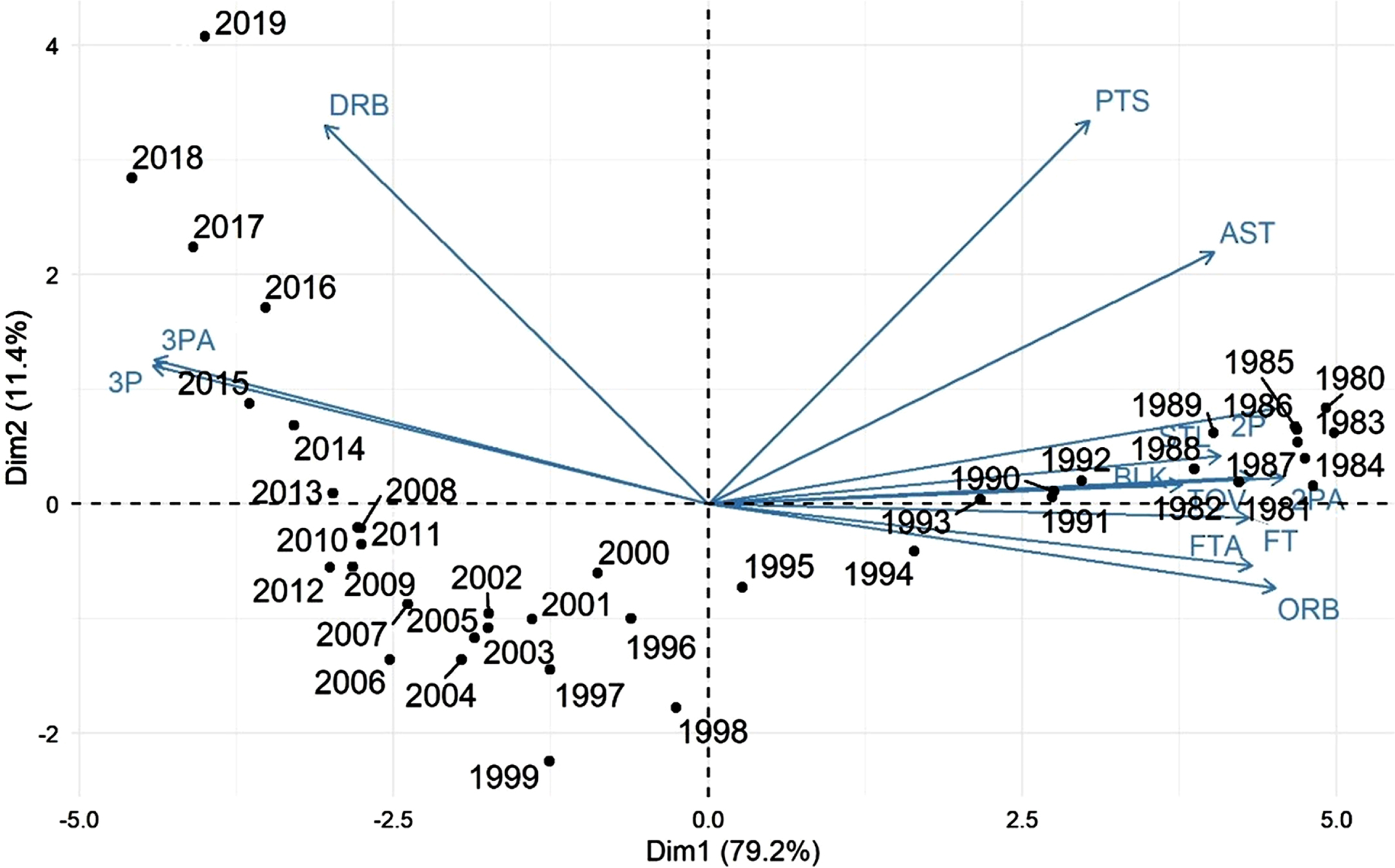
Firstly, a separation between two big groups can be noticed. Seasons from 1980 to 1994 are grouped on the right-hand side of the plot and the seasons from 1995 to 2019 are grouped on the left-hand side of the plot. On the right-hand side of Fig. 1, seasons between 1980 and 1994 are grouped with a large influence of offensive rebounds, turnovers, blocks, free throws and mainly two-point shots attempted and converted. Then, on the left-hand side of Fig. 1, two groups can be seen: on the bottom left of Fig. 1, the seasons from 1996 to 2013, and on the top left the seasons from 2014 to 2019. The top-left group is adjoining by defensive rebounds and three-point shots attempted and converted.
Figure 1 provides a visualization that makes clear the difference between the modern basketball strategies and those used in the ’80s and the ’90s. In the 1980s and beginning of the 1990s the number of three-point shots attempted would not reach ten per game, league’s offensive focus was completely near to the basket, hence, more opportunities were created for two-point shots, with the three-point line being an underused asset.
Figure 1 also emphasizes that the first seasons to depart from the right-hand side group are 1995, 1996, and 1997. Since, in 1995, searching for an incentive to franchises to attempt more shots from behind the three-point line, the NBA had the line distance reduced, finally raising the outside attempts to above ten per game. The line was moved back to its original position in 1997, and, as mentioned before, that year marks the seasons that began to deviate from a style of basketball focused on two-point shots, and slowly approximate to the left-hand side group, that along the years goes towards the three-point line focus, seen in the today’s NBA. This is visible in Fig. 1.
The period between 1995 and 2013 marks a transitional Era for the NBA, from the inside of the arc to the outside, moving towards the more recent years (2014–2019) where franchises are more interested in shots beyond the three-point line. It should be pointed out that the trend is not towards the extinction of the two-point shot, but to better game planning shot attempts. Teams started to choose better their shot attempts by distance, therefore being more efficient in scoring. For instance, long two-point shots, close to the three-point line but inside it, should be replaced for a three-point shot which has a better reward because of its distance.
Figure 2 helps to better understand strategy change in the NBA throughout the years, by showing the behavior of the proportion of shots attempted by distance: 1 to 3 feet, 3 to 10 feet, 10 to16 feet, 16 to the three-point line, and three-point shot (distances chosen as available in track data). From 2001 to 2019 (shooting track data only available from 2000-01).
Fig. 2
Shot proportion based on the distance to the basket, from 2001 to 2019.
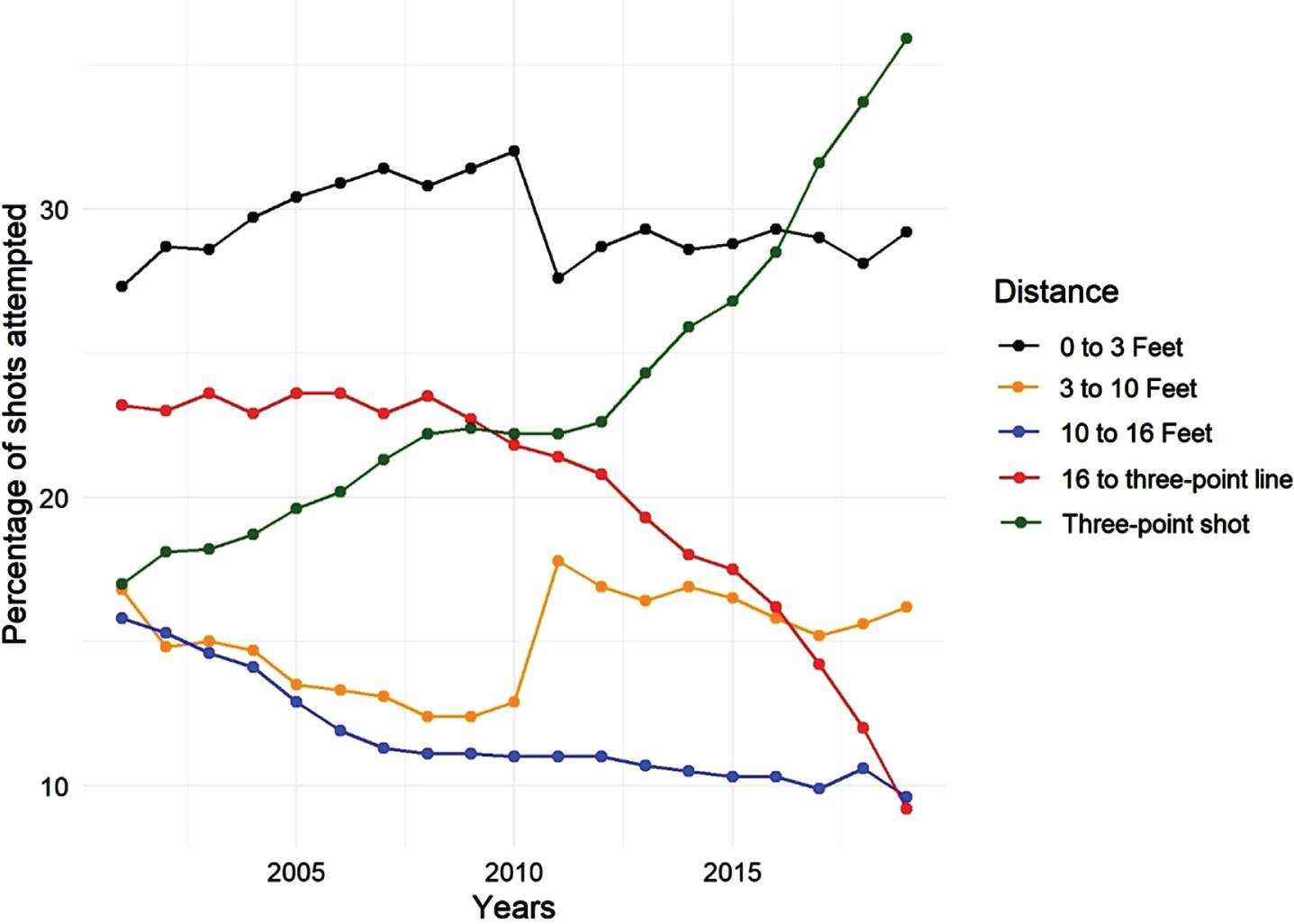
When analyzing Fig. 2, it becomes clear that teams are increasingly preferring three-point shots, and attempting less long two-point shots, especially from sixteen feet to the three-point line (23.75 feet at the top and 22 feet at the corners). Shots between zero and three feet have maintained their share around thirty percent for being extremely efficient shots, but it is also noticeable that in recent years the three-point proportion has surpassed the close shots proportion, showing a change in the NBA’s offensive focus. The redistribution is caused by the efficiency of the shot and its scoring capacity. Table 2 shows the average percentage of shots converted per distance from 2001 to 2019.
Table 2
Average percentage of shots converted per distance, from 2001 to 2019
| Shot Distance | Average percentage of shots converted |
| 0 to 3 feet | 62.09% |
| 3 to 10 feet | 39.36% |
| 10 to 16 feet | 39.58% |
| 16 to the three-point line | 39.87% |
| Three-point line | 35.60% |
As shown in Table 2, in a distance between zero and three feet, teams tend to score close to 62%of attempts, between three and ten feet, ten and sixteen feet and sixteen feet to the three-point line they succeed in about 39%of their attempts, and from the three-point line scoring percentage is close to 35%. When analyzing only these percentages, it might seem that shot attempts between three feet and the three-point line are more successful than behind the three-point line. However, considering the expected value (i.e., the expected number of points obtained) of each shot, it becomes clear why the NBA teams are turning their focus to the outside shots. Figure 3 exhibits the expected number of points per shot, calculated by multiplying the average scoring percentage by each shot value.
Fig. 3
Expected number of points per shot for each distance from 2001 to 2019.
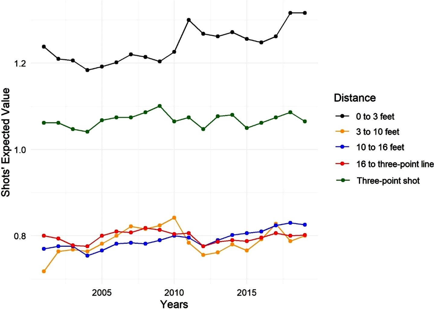
Analyzing Fig. 3, only close shots (from zero to three feet) and three-point shots create more than one point per shot, and the long two-point shots create around 0.8 points per shot. For this reason, it has become more rewarding for teams to attempt three-point shots than long two-point shots, once again reinforcing the change in the league’s focus.
Although even that it is better to attempt a three-point shot than long two-point shots, teams should not exclude any kind of shot. From a strategy point of view, removing any offensive artifice would make the offense more predictable for defensive game plans, and to completely stop to attempt mid-range shots would do exactly this.
Nowadays, there are plenty of players who are mid-range specialists, being extremely efficient in these long two-point shots. The strategy change that is happening in the NBA is to maximize the effect of its players when in the court. As a result, efficient mid-range players should keep attempting their shots, and inefficient players should be redirected to other shots that may be more effective.
Another noticeable change that can be seen in Fig. 1 is that from 1980 to 1994, the offensive rebounds are a more memorable presence and as years go by defensive rebounds become more important. Figure 4 shows the behavior of the average number of rebounds throughout the years. The number of defensive rebounds has increased from 1980 to 2019 and the number of offensive rebounds has decreased. This is a direct response to the offensive focus change in the NBA.
Fig. 4
Offensive and defensive rebounds averages, from 1980 to 2019.
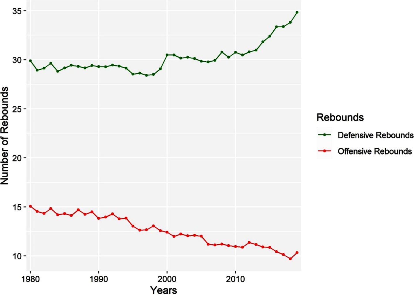
Shots attempted closer to the rim tend to maximize chances for a team to recover offensive rebounds and, as distance increases, it becomes more difficult for the offense to get rebounds, favoring defensive rebounds (Maheswaran et al., 2012). This does not suggest that attempting shots from near the rim or far from it generates rebounds for a team. Instead, it suggests that shot distance does influence a team’s rebounding chances, which is reflected in the rebounding numbers over the years (Fig. 4) because teams are willing to take distant shots (three-point shots) more frequently as the year’s progress. Maheswaran et al. (2012) also suggested that offensive rebounds are more difficult to recover in mid-range shots, but in three-point shots, it becomes relatively easier to gather offensive rebounds when compared to mid-range. This, once again, reinforces strategy change in the NBA: a good shot selection, especially choosing the right players to attempt long two-point shots should help a team become more efficient in scoring, also maximize its offensive opportunities and minimize other teams’ defensive opportunities.
3.2Stage 2: Cluster analysis –Seasons from 1980 to 2019
Subsequently to the PCA presented above, a k-means cluster analysis was implemented to reinforce and complement the results presented in Stage 1. Based on the gap statistic method, which uses the output of the clustering algorithm and compares the change in within-cluster dispersion with that expected under and appropriate reference null distribution (Tibshirani et al., 2001), three clusters were considered for the analysis (Fig. 5).
Fig. 5
K-means cluster analysis for all NBA seasons, from 1980 to 2019.
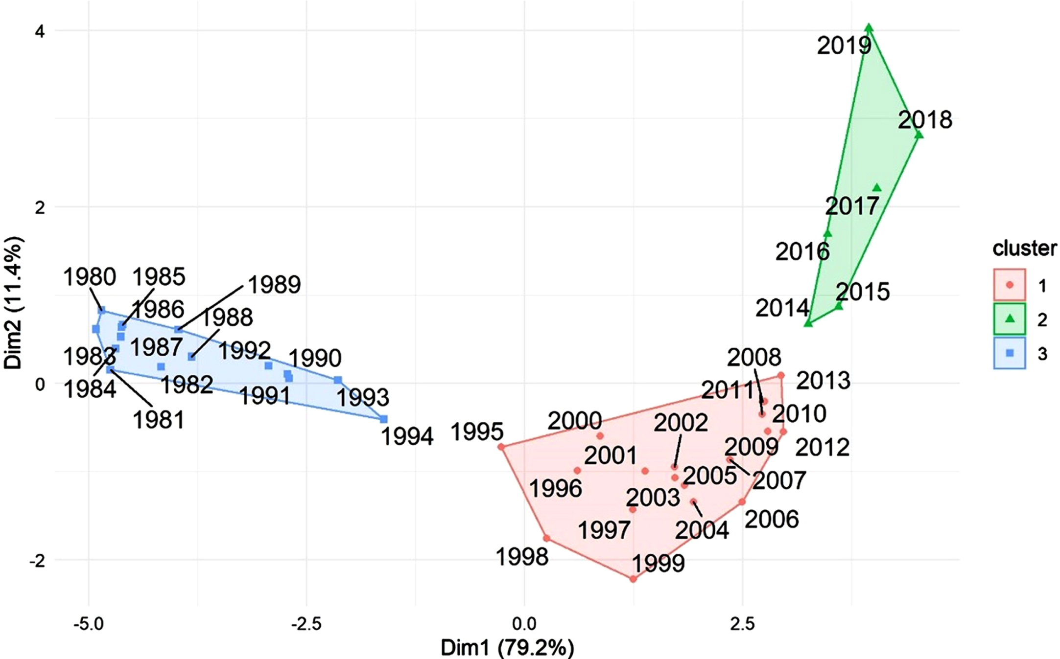
The cluster analysis depicted in Fig. 5 confirms and reinforces results obtained in Stage 1: seasons between 1980 and 1994 are grouped, seasons from 1995 to 2013 have similar behavior and are group together, and seasons from 2014 to 2019 form their cluster. Accordingly, and based on the interpretations discussed above, we name these groups, respectively, as Classic Era of the NBA, Transitional Era of the NBA, and Modern Era of the NBA. With the “Classic Era of the NBA” being associated with strategy and style similar to the years before the invention of the three-point line, more focused near the rim. The “Transitional Era of the NBA” suggests that during and after the NBA’s incentive reducing the three-point line distance, teams noticed the impact that attempts from the outside could have in games, causing a game-strategy transition. Lastly, the “Modern Era of the NBA”, is recognizable by a strong presence outside the arc, in ways never seen before.
Figures 6 and 7 present the increase of three-point shot attempts per game and decrease of two-point shot attempts per game in the NBA over the years, respectively. They indicate further evidence of the offensive focus change, confirming what was concluded in Stage 1 and, consequently, changing factors that contribute to a team’s regular season success.
Fig. 6
Three-point shot attempts per game, from 1980 to 2019.
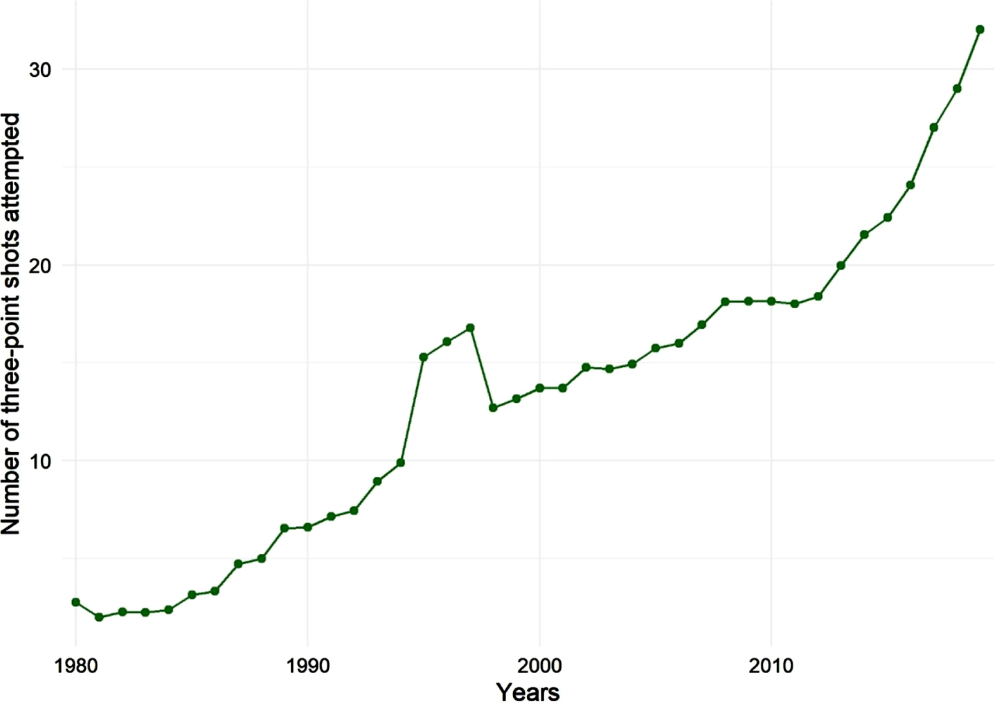
Fig. 7
Two-point shot attempts per game, from 1980 to 2019.
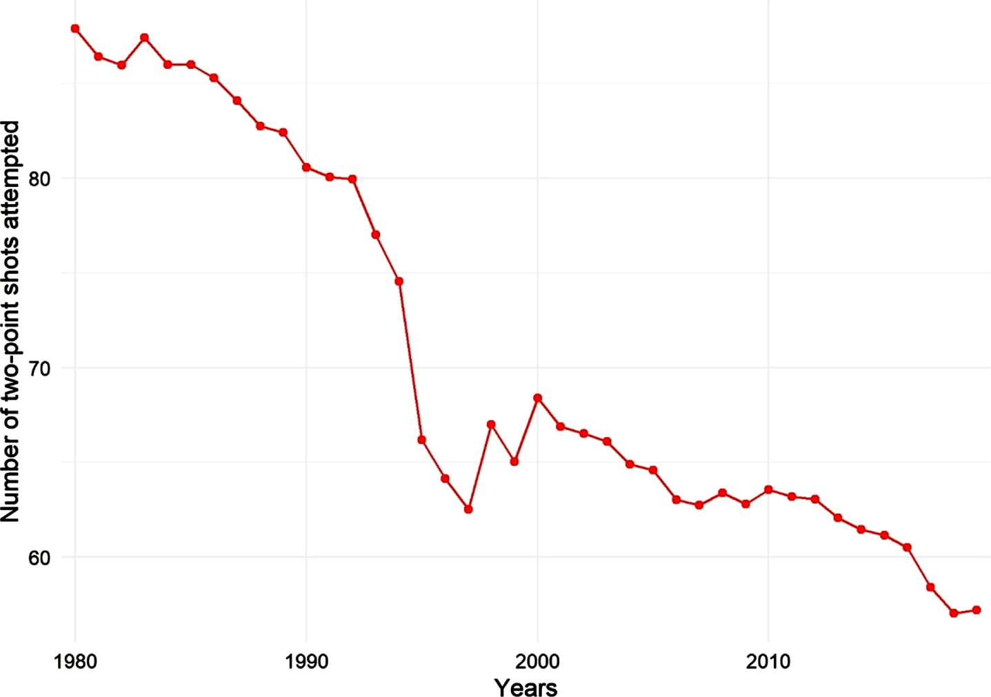
Figure 6 shows an abnormal increase in the shot attempts between 1995 and 1997, which are exactly the years that three-point line distance reduction was implemented by the NBA. After that period is possible to observe a sudden decrease, obviously caused by the return of the line to its original distance, followed by an expected growth as teams started to value more the outside shot opportunities.
Figure 7 is complementary to Fig. 6. It shows that two-point shot attempts drop from almost ninety per game in 1980 to close to sixty per game in 2019. Inefficient two-point shots are being replaced by more rewarding three-point shots. In fact, three-point shot attempts increased from less than five per game in 1980 to almost thirty-five per game in 2019 (Fig. 6).
In summary, Stages 1 and 2 highlight trends of the seasons throughout the years, where clusters of seasons can be associated with different Eras.
3.3Stage 3 –Principal component analysis –Winning teams
Stage 3 of this study aims at verifying whether teams with the best regular season record for each year of the regular seasons, i.e., teams that have won the most in their respective seasons, behave in the same manner as their respective seasons discussed in Stage 1.
Figure 8 shows the biplot with the first two principal components, explaining a total of 68.5%of the variability in data presented in Table 3. Figure 8 has noticeable similarities with Fig. 1. Teams with the best regular season record from 1980 to 1994 are grouped similarly as the seasons themselves, i.e., influenced by two-point shots attempted and converted, offensive rebounds, turnovers, and free throws attempted. The best teams in the regular season between 1995 and 2013 are in the transitional area, migrating from the right-hand (classical Era) to the left-hand (modern Era), changing style and strategy to a more outside/three-point focus. Lastly, in the top left-hand of Fig. 8, is possible to find teams from 2014 to 2019 grouped and characterized by defensive rebounds and three-point shots attempted and converted.
Fig. 8
Biplot with the first two principal components, considering the data for all regular season winning teams, from 1980 to 2019.
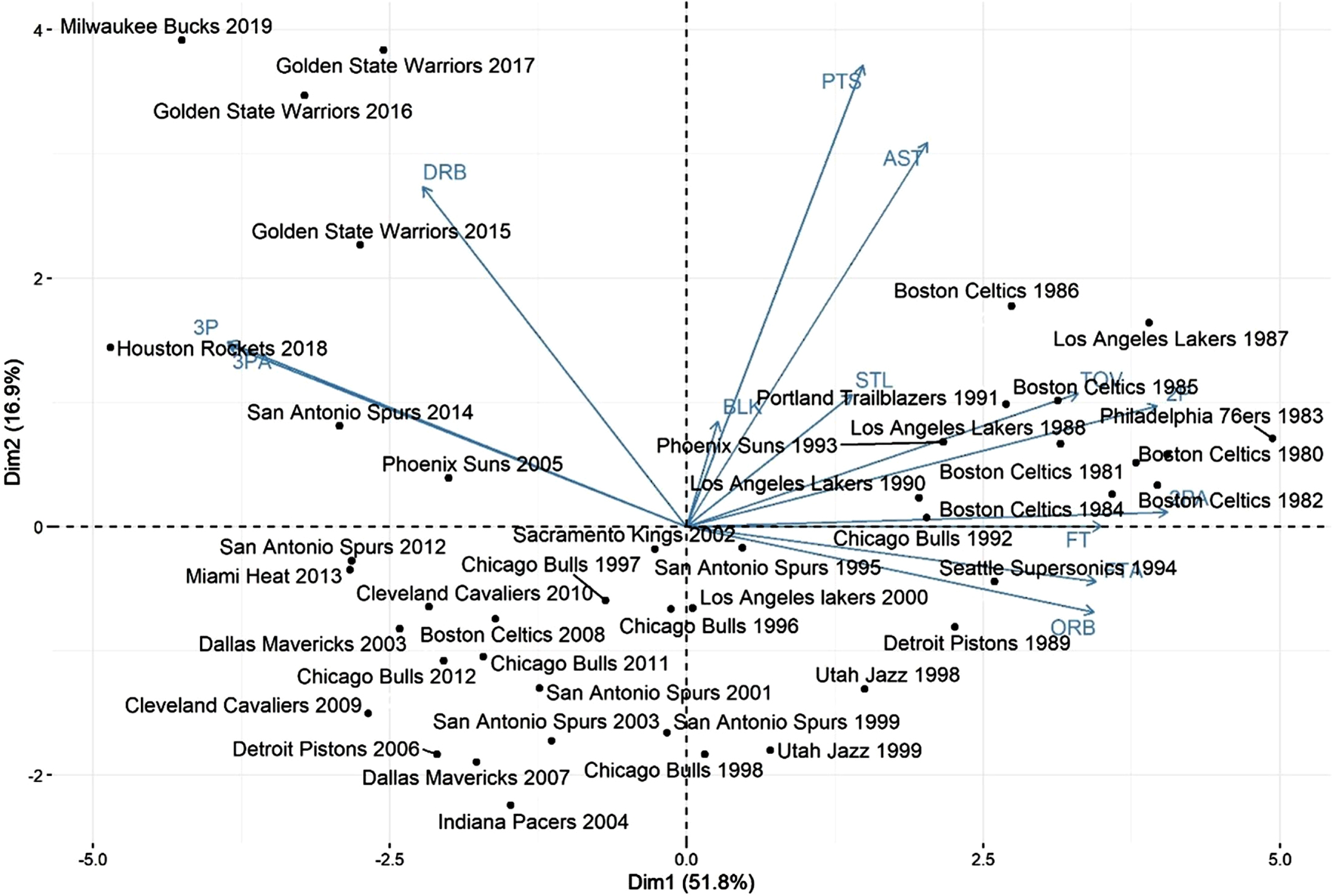
Table 3
First six rows of the data set that contains the teams with the best regular season records from 1980 to 2019
| Tm | 2P | 2PA | 3P | 3PA | FT | FTA | ORB | DRB | AST | STL | BLK | TOV | PTS |
| Milwaukee Bucks 2019 | 29.9 | 52.9 | 13.5 | 38.2 | 17.9 | 23.2 | 9.3 | 40.4 | 26.0 | 7.5 | 5.9 | 13.9 | 118.1 |
| Houston Rockets 2018 | 23.4 | 41.9 | 15.3 | 42.3 | 19.6 | 25.1 | 9.0 | 34.5 | 21.5 | 8.5 | 4.8 | 13.8 | 112.4 |
| Golden State Warriors 2017 | 31.1 | 55.8 | 12.0 | 31.2 | 17.8 | 22.6 | 9.4 | 35.0 | 30.4 | 9.6 | 6.8 | 14.8 | 115.9 |
| Golden State Warriors 2016 | 29.4 | 55.7 | 13.1 | 31.6 | 16.7 | 21.8 | 10.0 | 36.2 | 28.9 | 8.4 | 6.1 | 15.2 | 114.9 |
| Golden State Warriors 2015 | 30.8 | 60.0 | 10.8 | 27.0 | 16.0 | 20.8 | 10.4 | 34.3 | 27.4 | 9.3 | 6.0 | 14.5 | 110.0 |
| San Antonio Spurs 2014 | 32.0 | 62.0 | 8.5 | 21.4 | 15.7 | 20.0 | 9.3 | 34.0 | 25.2 | 7.4 | 5.1 | 14.4 | 105.4 |
*Teams (TM), Three-point shots attempted (3PA), Three-point shots converted (3P), Two-point shots attempted (2PA), Two-point shots converted (2P), Free throws attempted (FTA), Free throws converted (FT), Offensive rebounds (ORB), Defensive Rebounds (DRB), Assists (AST), Steals (STL), Blocks (BLK), Turnovers (TOV)) and Points scored (PTS).
Similarities between seasons’ and best regular-season teams are great results that help to reinforce the NBA’s Eras.
3.4Stage 4 –Cluster analysis –Winner teams
Stage 4 concludes the first part of this study, by performing a k-means clustering analysis to data from the best regular season teams (Table 3). The number of clusters, based on the Stage 2 analysis and the gap statistic method (Tibshirani et al., 2001), was set to three (Fig. 9).
Fig. 9
K-means cluster analysis for all winning teams, from 1980 to 2019.
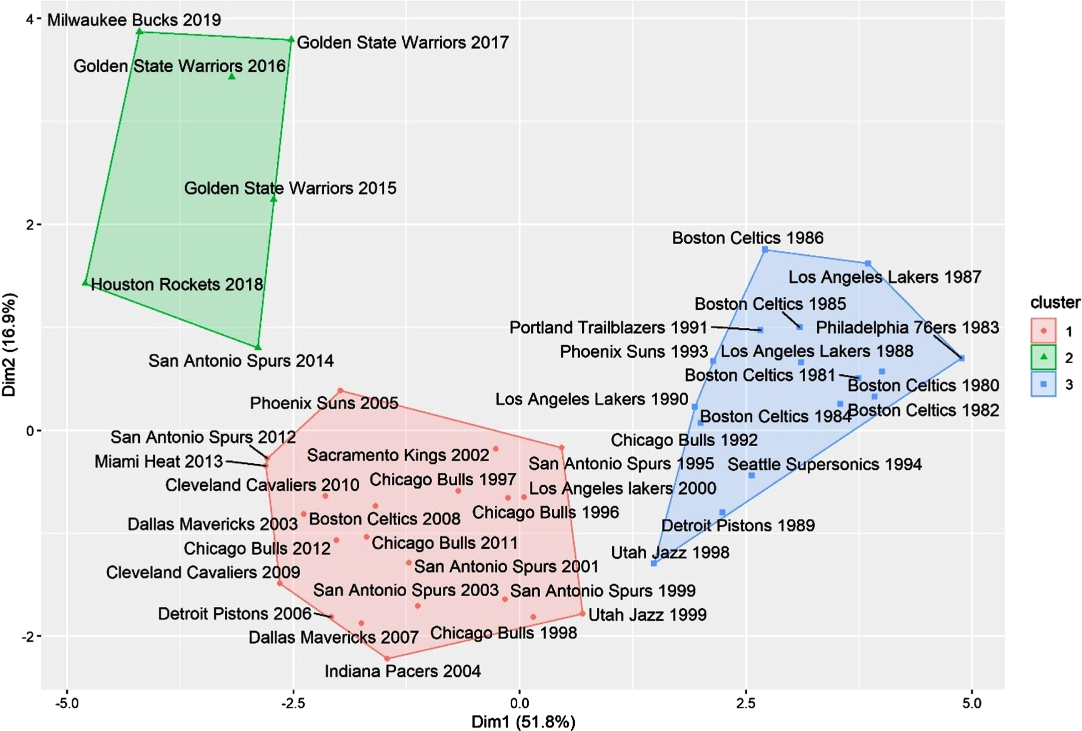
By analyzing the k-means cluster analysis shown in Fig. 9, it becomes clear its similarity to Fig. 5, resulting in a similar interpretation. It is also possible to notice that in two different seasons two teams had the same winning record, making them both the best team in their respective regular seasons. In 1999, the San Antonio Spurs and the Utah Jazz achieved the same record, and in 2012, the same thing has happened with the Chicago Bulls and the San Antonio Spurs. These pairs were grouped in their clusters.
In summary, Stages 3 and 4 reinforce results obtained in Stages 1 and 2, showing that teams that had the most success in their regular season are grouped similarly as their respective seasons.
3.5Stage 5 –LASSO regression –All seasons
In this last stage, we explore the effects of each variable on the number of victories of a given team in each season. For that, we would fit the multiple linear regression model of equation (1) for each year, resulting in 40 models. The data used in this analysis are displayed in Table 1, although all data used in this Stage was standardized. However, since many of the fitted models have shown high levels of multicollinearity, we decided to use the LASSO (Least Absolute Shrinkage and Selection Operator) regression. The LASSO regression allows performing both variable selection and model regularization to enhance the interpretability of the resulting models (Tibshirani, R., 1996). The optimal lambda value (see equation (2)) was determined with the “glmnet” package (Friedman et al., 2010) in software R (R Core Team, 2020).
The significant variables for each model were selected by the LASSO regression variable selection. The results of Stage 5 will be presented in Tables 4–6, as only the estimated beta coefficients for the models’ significant variables will be shown. The non-significant variables will have a “-“, where is supposed to have an estimated beta coefficient.
Starting with the Classical Era of the NBA, period from 1980 to 1994, Table 4 shows the beta coefficients for each covariate in each regression model/year.
Table 4
Estimated Beta coefficients for each significant covariate in the LASSO regressions, for the years associated with the Classical Era of the NBA (1980–1994)
| Year | 2P | 2PA | 3P | 3PA | FT | FTA | ORB | DRB | AST | STL | BLK | TOV | PTS |
| 1980 | 0.249 | –1.197 | – | –0.233 | – | –0.156 | 0.535 | 0.576 | 0.067 | 0.461 | 0.102 | –0.618 | 0.712 |
| 1981 | 0.284 | –0.412 | – | 0.157 | – | – | 0.176 | 0.288 | 0.246 | 0.280 | 0.178 | –0.061 | 0.146 |
| 1982 | 0.145 | –0.406 | – | –0.083 | – | 0.156 | 0.332 | 0.505 | 0.253 | 0.414 | 0.136 | –0.336 | – |
| 1983 | 0.274 | –0.753 | – | –0.148 | – | 0.158 | 0.211 | 0.353 | 0.271 | 0.460 | 0.145 | –0.487 | – |
| 1984 | – | – | – | – | 0.008 | – | – | – | – | – | – | – | – |
| 1985 | – | –0.883 | – | –0.144 | 0.249 | –0.543 | 0.610 | 0.308 | 0.361 | 0.366 | 0.303 | –0.484 | 0.413 |
| 1986 | – | –0.440 | – | – | 0.065 | –0.067 | 0.261 | 0.254 | 0.447 | 0.345 | 0.284 | –0.419 | 0.233 |
| 1987 | 0.180 | –0.516 | – | –0.150 | 0.080 | – | – | 0.487 | – | 0.291 | 0.191 | –0.424 | 0.245 |
| 1988 | 0.305 | –0.499 | – | – | 0.253 | – | 0.032 | 0.248 | – | 0.214 | 0.103 | –0.486 | 0.049 |
| 1989 | – | –0.101 | – | – | 0.425 | – | – | 0.023 | – | – | – | –0.109 | 0.174 |
| 1990 | 0.668 | –1.126 | – | – | – | 0.070 | 0.394 | 0.382 | 0.021 | 0.220 | 0.050 | –0.396 | – |
| 1991 | 0.713 | –1.409 | – | –0.273 | – | 0.119 | 0.596 | 0.467 | 0.136 | 0.228 | –0.022 | –0.359 | – |
| 1992 | 0.815 | –1.288 | –0.947 | 0.678 | 0.008 | –0.159 | 0.392 | 0.172 | 0.169 | –0.127 | 0.109 | 0.087 | 0.448 |
| 1993 | 0.622 | –0.931 | 0.299 | –0.433 | –0.002 | –0.099 | 0.293 | 0.723 | –0.129 | 0.474 | –0.056 | –0.430 | – |
| 1994 | 0.489 | –0.844 | – | –0.266 | –0.002 | – | 0.314 | 0.512 | 0.104 | 0.366 | –0.040 | –0.327 | – |
*Three-point shots attempted (3PA), Three-point shots converted (3P), Two-point shots attempted (2PA), Two-point shots converted (2P), Free throws attempted (FTA), Free throws converted (FT), Offensive rebounds (ORB), Defensive Rebounds (DRB), Assists (AST), Blocks (BLK), Turnovers (TOV) and Points scored (PTS).
From the analysis of Table 4, it is possible to observe that two-point shots converted (2P), as expected, are important to win regular season games in this era. On the contrary, three-point shots converted (3P) are not significant in most years, only appearing significantly in the final years. The two-point shot attempts (2PA) are an important factor to win games in the regular season, although it negatively influences the number of wins.
Analyzing variables 2P and 2PA, it is possible to attribute these negative beta coefficients, in 2PA’s case, to a good two-point shot percentage. In other words, to win games teams must convert two-point shots at a high rate, keeping attempts to a minimum and conversion to a maximum. The same pattern can be found when we analyze variables related to three-point shots (3P/3PA), i.e., in most years the three-point shot attempts (3PA) have negatively influenced the number of wins. In 1992’s case, 3P’s beta coefficient is negative (Table 5), meaning that the greater the number of shots converted, the worse the team’s win record in the regular season. One explanation for this might be related to the fact that in this era, teams used to have low numbers of outside shots attempted per game (e.g., in 1992 teams only tried an average of 7.6 three-point shots per game, converting only 2.5 of them). Thus, a greater number of three-points converted (3P) would require a much higher number of attempts (3PA), which was not compatible with this era’s style of play. The lack of recognition of the three-point shot as a valuable asset contributes to this negative beta coefficient. In 1993, a great number of converted shots (3P) helped winning more games, and a great number of attempted shots (3PA) did not, even in an era that the three-point shot was underrated.
Table 5
Estimated Beta coefficients for each significant covariate in the LASSO regressions, for the years associated with the Transitional Era of the NBA (1995–2013)
| Year | 2P | 2PA | 3P | 3PA | FT | FTA | ORB | DRB | AST | STL | BLK | TOV | PTS |
| 1995 | –0.001 | –0.718 | 0.565 | –1.060 | –0.193 | 0.167 | 0.376 | 0.326 | 0.318 | 0.195 | –0.053 | –0.338 | 0.266 |
| 1996 | –0.088 | –1.385 | – | –1.268 | –0.272 | –0.073 | 0.548 | 0.457 | 0.013 | 0.283 | –0.016 | –0.403 | 0.914 |
| 1997 | – | –1.429 | 0.037 | –0.996 | –0.120 | –0.167 | 0.393 | 0.434 | 0.007 | 0.225 | 0.052 | –0.276 | 0.694 |
| 1998 | 0.329 | –1.338 | – | –0.703 | –0.002 | –0.127 | 0.427 | 0.401 | 0.247 | 0.403 | –0.026 | –0.423 | 0.043 |
| 1999 | 0.242 | –1.283 | – | –0.611 | – | – | 0.396 | 0.587 | 0.145 | 0.289 | – | –0.429 | 0.195 |
| 2000 | 0.410 | –0.746 | – | –0.452 | –0.014 | –0.071 | –0.030 | 0.431 | 0.150 | 0.249 | – | –0.396 | 0.089 |
| 2001 | 0.554 | –0.950 | – | –0.308 | – | 0.008 | 0.078 | 0.390 | – | 0.333 | – | –0.446 | 0.103 |
| 2002 | 0.540 | –0.910 | – | –0.406 | 0.506 | –0.516 | 0.138 | 0.314 | –0.012 | 0.494 | 0.341 | –0.688 | – |
| 2003 | – | –1.757 | 0.027 | –1.591 | –0.312 | –0.145 | 0.484 | 0.523 | 0.081 | 0.325 | –0.105 | –0.575 | 0.883 |
| 2004 | 3.922 | –1.758 | 3.844 | –1.622 | 1.705 | –0.247 | 0.511 | 0.364 | 0.225 | 0.383 | 0.117 | –0.694 | –3.719 |
| 2005 | –0.229 | –1.811 | – | –1.651 | –0.008 | –0.194 | 0.552 | 0.633 | 0.254 | 0.489 | –0.040 | –0.341 | 0.731 |
| 2006 | 0.423 | –1.098 | 1.673 | –2.258 | 0.173 | –0.024 | 0.407 | 0.600 | 0.323 | 0.223 | 0.103 | –0.628 | –0.053 |
| 2007 | – | –1.020 | 0.073 | –1.474 | –0.147 | –0.315 | 0.478 | 0.517 | 0.078 | 0.224 | 0.093 | –0.588 | 0.921 |
| 2008 | – | –1.364 | – | –1.184 | 0.043 | –0.377 | 0.529 | 0.420 | 0.047 | 0.309 | 0.071 | –0.356 | 0.794 |
| 2009 | –0.856 | –1.187 | –0.034 | –1.871 | –0.501 | –0.134 | 0.366 | 0.494 | 0.146 | 0.417 | –0.033 | –0.446 | 1.361 |
| 2010 | – | –0.857 | – | –0.592 | 0.091 | – | 0.382 | 0.495 | 0.236 | 0.220 | 0.044 | –0.476 | 0.278 |
| 2011 | 0.082 | –1.585 | –0.162 | –1.069 | 0.005 | –0.366 | 0.417 | 0.485 | 0.126 | 0.315 | 0.140 | –0.387 | 0.563 |
| 2012 | – | – | – | – | – | – | – | 0.434 | – | 0.123 | – | – | 0.249 |
| 2013 | – | –1.325 | 0.632 | –1.648 | 0.161 | –0.341 | 0.570 | 0.441 | 0.191 | 0.444 | – | –0.361 | 0.374 |
*Three-point shots attempted (3PA), Three-point shots converted (3P), Two-point shots attempted (2PA), Two-point shots converted (2P), Free throws attempted (FTA), Free throws converted (FT), Offensive rebounds (ORB), Defensive Rebounds (DRB), Assists (AST), Blocks (BLK), Turnovers (TOV) and Points scored (PTS).
Offensive (ORB) and defensive rebounds (DRB), assists (AST), blocks (BLK), and steals (STL) are significant factors, influencing mostly in a positive way. However, turnovers (TO), have a negative influence on the number of wins.
An unexpected result was obtained for 1984, which only has one significant covariable, with an exceptionally low coefficient. This means that for that year, none of the considered covariates, except free-throws-made (FT), can explain the number of regular season wins.
Moving to the Transitional era of the NBA (1995–2013), Table 5 shows the beta coefficients for each covariate in each regression model/year.
During this era, three (3PA) and two-point shot attempted (2PA) and converted (2P) influenced the number of wins in the same way as they have in the previous era. However, in some years the number of two-point shots converted (2P) was not a significant factor. The beginning of this era is marked by the three-point line distance reduction (1995–1997) to incentivize teams to create more opportunities from behind the arc. This change resulted in three-point shots converted (3P) being significant in two out of three years of the distance reduction, a tendency that appears more strikingly after 2002, being significant in several years. Yet, it is possible to see that the three-point shots converted (3P) are non-significant or a negative influence on the number of wins, which confirms the gameplay style transition that was observed in the previous stages of this study.
Another unexpected result was obtained for 2012, where the three-point shots (3P/3PA) and the two-point shots (2P/PA) were non-significant factors to explain the response variable. However, the number of points scored (PTS) was a significant factor to explain the number of wins.
Offensive (ORB) and defensive rebounds (DRB), assists (AST), steals (STL), blocks (BLK), and turnovers (TO) are solid factors to explain the number of regular seasons wins, throughout the entire era.
Lastly, Table 6 shows the beta coefficients for each covariate in each regression model/year for the Modern Era of the NBA.
Table 6
Estimated Beta coefficients for each significant covariate in the LASSO regressions, for the years associated with the Modern Era of the NBA (2014–2019)
| Year | 2P | 2PA | 3P | 3PA | FT | FTA | ORB | DRB | AST | STL | BLK | TOV | PTS |
| 2014 | 0.088 | –1.440 | – | –0.999 | – | –0.381 | 0.497 | 0.683 | 0.137 | 0.249 | – | –0.367 | 0.478 |
| 2015 | 0.553 | –1.643 | –0.154 | –0.634 | 0.893 | –0.905 | 0.279 | 0.579 | 0.135 | 0.545 | 0.031 | –0.532 | – |
| 2016 | –4.861 | –1.426 | –5.871 | –1.748 | –1.999 | –0.282 | 0.592 | 0.538 | 0.116 | 0.537 | 0.025 | –0.588 | 4.986 |
| 2017 | – | –1.620 | 0.279 | –1.451 | –0.298 | – | 0.551 | 0.364 | 0.043 | 0.426 | 0.042 | –0.511 | 0.572 |
| 2018 | – | –1.275 | – | –1.148 | – | –0.420 | 0.307 | 0.408 | –0.170 | 0.308 | 0.100 | –0.303 | 0.808 |
| 2019 | – | –1.446 | 0.407 | –1.653 | –0.099 | –0.091 | 0.384 | 0.501 | 0.071 | 0.293 | –0.018 | –0.386 | 0.618 |
*Three-point shots attempted (3PA), Three-point shots converted (3P), Two-point shots attempted (2PA), Two-point shots converted (2P), Free throws attempted (FTA), Free throws converted (FT), Offensive rebounds (ORB), Defensive Rebounds (DRB), Assists (AST), Blocks (BLK), Turnovers (TOV) and Points scored (PTS).
In the Modern Era, an interesting change is noticeable in two-point shots converted (2P). In 2014 and 2015 this covariate influenced positively the number of regular season wins, in 2016 had a negative influence, and after 2016, it stopped to be a significant factor.
These changes, as expected, show that the number of two-point shots attempted (2PA) and converted (2P) are an aspect of the game that should be carefully controlled, i.e., a better shot selection, previously mentioned in this study, is key to win games.
Simultaneously, the three-point shots converted (3P) are a relevant factor at the beginning of the Modern Era, however, with a negative influence in 2015 and 2016, probably a reflex of the Transitional Era. In 2017 and 2019, the three-point shots converted (3P) started to contribute positively to the game outcome.
Offensive (ORB) and defensive (DRB) rebounds, assists (AST), steals (STL), blocks (BLK), free-throws attempted (FTA), turnovers (TO), and points (PTS) also are significant factors throughout the whole Modern Era.
In summary, the results shown in Tables 4–6 reinforce the definition of the three Eras of NBA, provide further insights for individual seasons, and define the significant covariates to predict a team’s number of regular season wins.
4Concluding remarks
In this paper, we were interested in characterizing NBA’s gameplay along the time to identify trends, success factors, and group seasons, and winning teams into clusters of common characteristics and gameplay behavior. For that, we considered statistical methods such as the unsupervised machine learning techniques of principal component analysis and cluster analysis, and LASSO regression.
Based on that analysis for the game-related statistics of the NBA’s regular seasons, from 1979-80 to 2018-19, three main Eras can be defined. Between 1980 and 1994 is the Classic Era of the NBA, which is more focused on two-point shots, offensive rebounds, free throws, steals, and blocks. The LASSO regressions confirmed that a high number of two-point shots converted allied with a low number of attempts were a determinant factor to increase teams’ winning records in this period. This era is also influenced by many factors such as offensive and defensive rebounds, assists, blocks, turnovers, and steals. However, three-point shots converted are not significant factors in most years and a high number of three-point shots attempted decrease teams’ winning records.
From 1995 to 2013 is the Transitional Era of the NBA. During this era, it is possible to observe season’s behavior migrating from the rim to the arc, i.e., the offensive strategy was beginning to change, and the three-point shots were becoming a useful resource to win games. The LASSO regressions confirmed that two-point shots attempted and converted behave the same way as they did in the previous era, however it is possible to see some years having these variables as non-factors to win games. Simultaneously, three-point shots converted started to become significant factors to increase teams’ winning record, especially after 2002. Offensive and defensive rebounds, assists, steals, blocks and turnovers continue to explain the number of regular season wins in this era.
Lastly, from 2014 to 2019 is the Modern Era of the NBA, grouped by defensive rebounds, three-point shots attempted and converted. Once more, based on the LASSO regressions, it was confirmed that two-point shots converted started to be a negative factor to win games, and eventually became a non-factor. At the same time, three-point shots converted became positive factors to win games, which confirms the change that has been occurring in the modern NBA. Offensive and defensive rebounds, assists, steals, blocks, free-throws attempted, turnovers and points also continued to be important factors throughout the whole Modern Era.
All eras considered, it can be concluded that the variables that had more impact throughout all seasons were: two-point shots attempted, three-point shots attempted, offensive rebounds, defensive rebounds, assists, turnovers, blocks, steals, and points scored. It was also possible to identify the main differences between the three eras: Classic Era of the NBA focused on the inside the arc shots; Transitional Era of the NBA evidences the migration from the rim to the three-point line; and Modern Era of the NBA is characterized by the better shot selection, replacing inefficient two-point shots by more rewarding three-point shots.
Acknowledgments
The authors would like to thank the associate editor, the two anonymous reviewers whose suggestions helped to improve this manuscript, and the Research Support Foundation of the State of Bahia (FAPESB) for their financial support.
References
1 | Bradu, D. , & Gabriel, K. R. (1978) , The Biplot as a Diagnostic Tool for Models of Two-Way Tables. Technometrics, 20: (1), 47–68. doi: 10.1080/00401706.1978.10489617 |
2 | Chan, H. F. , Savage, D. A. ,& Torgler, B. (2019) , 2019, There and back again: Adaptation after repeated rule changes of the game. Journal of Economic Psychology, 75: , 102129. doi: 10.1016/j.joep.2018.12.003 |
3 | Fichman, M. , & O’Brien, J. R. (2019) , Optimal shot selection strategies for the NBA. Journal of Quantitative Analysis in Sports, 15: (3), 203–211. doi: 10.1515/jqas-2017-0113 |
4 | Friedman, J. , Hastie, T. , & Tibshirani, R. (2010) , “Regularization Paths for Generalized Linear Models via Coordinate Descent.”. Journal of Statistical Software, 33: (1), 1–22. https://www.jstatsoft.org/v33/i01/ |
5 | Gabriel, K. R. (1971) , The biplot graphic display of matrices with application to principal component analysis. Biometrika, 58: (3), 453–467. doi: 10.1093/biomet/58.3.453 |
6 | Gannaway, G. , Palsson, C. , & Price, J. (2014) , Technological Change, Relative Worker Productivity, and Firm-Level Substitution: Evidence From the NBA. Journal of Sports Economics, 15: (5), 478–496. doi: 10.1177/1527002514542740 |
7 | Goldsberry, K. P. (1978) , Sprawlball: A visual tour of the new era of the NBA. Boston: Houghton Mifflin Harcourt. |
8 | Gómez, M. A. , Lorenzo, A. , Sampaio, J. , Ibáñez, S. J. , & Ortega, E. (2008) , Game-related statistics that discriminatedwinning and losing teams from the Spanish men’s professionalbasketball teams. Collegium Antropologicum, 32: , 315–319. |
9 | Ibáñez, S. J. , Sampaio, J. , Feu, S. , Lorenzo, A. , Gómez, M. A. , & Ortega, E. (2008) , Basketball game-related statistics thatdiscriminate between teams’ season-long success. EuropeanJournal of Sport Science, 8: (6), 369–372. doi: 10.1080/17461390802261470 |
10 | Ibáñez, S. J. , Sampaio, J. , Sáenz-López, P. , Giménez, J. , & Janeira, M. A. , (2008) , Game statisticsdiscriminating the final outcome of Junior World BasketballChampionship matches (Portugal 1999). Journal of Human MovementStudies, 45: , 1–19. |
11 | Johnson R.A. & Wichern, D.W. , Applied Multivariate Statistical Analysis. 6th ed. USA: Pearson; (2007) . |
12 | Jolliffe, I.T. Principal component analysis. New York: Springer; (2002) . |
13 | Kubatko, J. , Oliver, D. , Pelton, K. , & Rosenbaum, D. T. (2007) , A Starting Point for Analyzing Basketball Statistics. Journal of Quantitative Analysis in Sports, 3: (3), 2007. doi: 10.2202/1559-0410.1070 |
14 | Maheswaran, R. , Chang, Y. , Henehan, A. , & Danesis, S. Deconstruction the Rebound with Optical Tracking Data, in MIT Sloan Sports Analytics Conference, 2012. |
15 | Oliver, D. (2011) , Basketball on paper: Rules and tools for performance analysis. Washington, D.C.: Potomac Books. |
16 | Özmen, M. U. (2016) , Marginal contribution of game statistics to probability of winning at different levels of competition in basketball: Evidence from the Euroleague. International Journal of Sports Science & Coaching, 11: (1), 98–107. doi: 10.1177/1747954115624828 |
17 | R Core Team, 2020, R: A language and environment for statistical computing. R Foundation for Statistical Computing, Vienna, Austria. URL: https://www.R-project.org/. |
18 | Sampaio, J. , & Janeira, M. (2003) , Statistical analyses of basketball team performance: Understanding teams’ wins and losses according to a different index of ball possessions. International Journal of Performance Analysis in Sport, 3: (1), 40–49. doi: 10.1080/24748668.2003.11868273 |
19 | Sampaio, J. , Janeira, M. , Ibáñez, S. , & Lorenzo, A. (2006) , Discriminant analysis of game-related statistics between basketballguards, forwards and centres in three professional leagues. European Journal of Sport Science, 6: (3), 173–178. doi: 10.1080/17461390600676200 |
20 | Sampaio, J. , Lago, C. , & Drinkwater, E. J. (2010) , Explanations for the United States of America’s dominance in basketball at the Beijing Olympic Games. Journal of Sports Sciences, 28: (2), 147–152. doi: 10.1080/02640410903380486 |
21 | Teramoto, M. , & Cross, C. L. (2017) , Importance of team height to winning games in the National Basketball Association. International Journal of Sports Science & Coaching, 13: (4), 559–568. doi: 10.1177/1747954117730953 |
22 | Tibshirani, R. (1996) , Regression shrinkage and selection via the lasso. Journal of the Royal Statistical Society: Series B (Methodological), 58: (1), 267–288. doi: 10.1111/j.2517-6161.1996.tb02080.x |
23 | Tibshirani, R. , & Walther, G. , & Hastie, T. (2017) , Estimating the number of clusters in a data set via the gap statistic. Journal of the Royal Statistical Society: Series B (Statistical Methodology), 63: (2), 411–423. doi: 10.1111/1467-9868.00293 |
24 | Trninic, S. , Dizdar, D. , & Luksic, E. (2017) , Differences between winning and defeated top quality basketball teams in final tournaments of European club championship. Collegium Antropologicum, 26: , 521–531. |


